Resolving the hot dust around HD69830 and $\eta$ Corvi with MIDI and VISIR

Abstract

Aims. Most of the known debris discs exhibit cool dust in regions analogous to the Edgeworth-Kuiper Belt. However, a rare subset show hot excess from within a few AU, which moreover is often inferred to be transient from models for planetesimal belt evolution. In this paper we examine 2 such sources to place limits on their location to help distinguish between different interpretations for their origin.

Methods. We use MIDI on the VLTI to observe the debris discs around $\eta$ Corvi and HD69830 using baseline lengths from 44–130m. New VISIR observations of HD69830 at 18.7$\mu$m are also presented. These observations are compared with disc models to place limits on disc size.

Results. The visibility functions measured with MIDI for both sources show significant variation with wavelength across 8–13$\mu$m in a manner consistent with the disc flux being well resolved, notably with a dip at 10–11.5$\mu$m due to the silicate emission feature. The average ratio of visibilities measured between 10–11.5$\mu$m and 8–9$\mu$m is 0.934$\pm$0.015 for HD69830 and 0.880$\pm$0.013 for $\eta$ Corvi over the four baselines for each source, a departure of 4 and 9$\sigma$ from that expected if the discs were unresolved. HD69830 is unresolved by VISIR at 18.7$\mu$m. The combined limits from MIDI and 8m imaging constrain the warm dust to lie within 0.05–2.4AU for HD69830 and 0.16–2.98AU for $\eta$ Corvi.

Conclusions. These results represent the first resolution in the mid-infrared of dust around main sequence stars. The constraints placed on the location of the dust are consistent with radii predicted by SED modelling (1.0AU for HD69830 and 1.7AU for $\eta$ Corvi). Tentative evidence for a common position angle for the dust at 1.7AU with that at 150AU around $\eta$ Corvi, which might be expected if the hot dust is fed from the outer disc, demonstrates the potential of this technique for constraining the origin of the dust and more generally for the study of dust in the terrestrial regions of main sequence stars.

1 Introduction

Debris discs are believed to be remnants of planet formation. As well as providing a unique window on how a system may have formed and evolved, studies of debris discs can reveal much about the current status of a system: the location of the dust can indicate possible configurations of any planetary system around the star (see e.g. Wyatt 2008); and the amount of debris material allows us to understand what physical conditions may be like for any habitable planets in the system (Greaves 2006). Debris disc emission is seen to peak typically longwards of 60$\mu$m implying that the dust is cool $<$80K and thus predicted to lie at regions many 10s AU from the star. In the majority of cases where this emission has been resolved around Sun-like stars it has been confirmed to lie at $>$40AU (see e.g., Holland et al. 1998; Greaves et al. 2005; Kalas et al. 2007). Exoplanet studies on the other hand typically probe close-in regions for giant planets, as most planets detected to date have been found through radial velocity techniques with their inherent detection biases (see e.g. Butler et al. 2006). Debris disc studies are therefore typically complementary to exoplanet studies. Furthermore, comparison with the Solar System’s debris discs, the asteroid and Edgeworth-Kuiper belts, can help us further understand the likelihood of finding Solar System analogues in our solar neighbourhood.

Very few stars exhibit hot dust within $\sim$10 AU, i.e. in the region where we expect planets may have formed (Ida & Lin 2004). Four surveys have searched for hot dust around Sun-like stars by looking for stars with a 25 $\mu$m flux in excess of photospheric levels using IRAS (Gaidos 1999), ISO (Laureijs et al. 2002) and Spitzer (Hines et al. 2006; Bryden et al. 2006). All concluded that only $2\pm 2$% of Sun-like stars have hot dust with infrared luminosities $f=L_{IR}/L_{\star}>10^{-4}$. These hot dust sources provide a unique opportunity to probe the terrestrial planet region of their systems (e.g. Wyatt 2002). Wyatt et al. (2007) identified 7 main-sequence Sun-like (F, G and K-type) sources with hot dust emission at $\sim$1AU. For these sources the levels of excess emission observed were compared with the predictions of analytical models for the collisional evolution of debris discs. This model predicts that there is a maximum level of emission that a disc of a given age and radius can have; discs that are initially more massive, which one may assume might end up brighter, process their mass through the cascade more quickly (i.e. more massive discs have shorter collisional timescales). Although Löhne et al. (2008) found that the analytical model may underestimate the levels of dust emission produced by debris discs at ages of $\ga$1Gyr by a factor of 10, they concurred with the findings of Wyatt et al. (2007) that for 4 of these 7 sources the level of dust emission is too high to be explained as the product of a steady-state collisional cascade in a planetesimal belt coincident with the dust at $\sim$1AU, and must therefore be the product of a transient event. Recent near-infrared interferometric observations have also revealed 4 systems with hot dust emission at $\sim$0.1AU from the star (Vega, Absil et al. 2006; $\tau$ Ceti, di Folco et al. 2007; $\beta$ Leo and $\zeta$ Lep, Akeson et al. 2009, although the hot emission around $\zeta$ Lep must be confirmed). Dust lifetimes in these regions are very short and these dust populations are also likely to have been produced in a recent transient event.

A critical diagnostic to understand the origin of this transient emission is the location of the disc, and in particular whether the emission is asymmetric. In this paper we examine two sources inferred to have transient emission at $\sim$1AU, HD69830, a K0V-type star with an age of 2Gyr (Beichman et al. 2006) and $\eta$ Corvi, an F2V-type star with an age of 1.3Gyr (Mallik et al. 2003). The predicted dust locations around both sources is 80–90 mas (from SED modelling of the IRS spectra of the targets, Beichman et al. 2005; Chen et al. 2006), although there remains considerable uncertainty in the true radial location of the emission. Thus far 8m imaging of $\eta$ Corvi suggests the dust lies within 3AU of the star (Smith et al. 2008). Here we present VISIR observations of HD69830 and MIDI observations of both targets.

This paper is structured as follows. In section 2 we describe our interferometric observations and data reduction procedures. In section 3 we describe the results of the MIDI observations. In section 4 we present new VISIR imaging of HD69830 showing that the excess emission at 18.72$\mu$m is not-extended, and discuss the implications for the maximum extent of the disc. In section 5 we discuss the results and the implications for the radial location of the debris discs. We conclude in section 6.

Table 1: Characteristics of the science and calibration targets.

Science targets
Source	Spec type	Age	RA	Dec	$F_{\ast}$ at 10$\mu$m	$F_{disc}$ at 10$\mu$m	Predicted disc size
HD		Gyr			mJy	mJy	mas
69830	K0V	2a	08 18 23.95	-21 37 55.8	872	102	80
$\eta$ Corvi	F2V	1.3b	12 32 04.23	-16 11 45.6	1736	371	90
Calibrators
Source	Spectral type		RA	Dec	$F_{\ast}$ at 10 $\mu$m		Angular size
HD					mJy		mas
61935	G9III		07 41 14.83	-09 33 04.10	9490		2.24$\pm$0.01
73840	K3III		08 40 01.47	-12 28 31.30	12312		2.40$\pm$0.01
95272	K1III		10 59 46.46	-18 17 55.56	9510		2.24$\pm$0.01
116870	K5III		13 26 43.17	-12 42 27.60	10416		2.58$\pm$0.01
107218	M4III		12 19 42.59	-19 11 55.97	7913		2.16$\pm$0.02

For science targets the stellar flux was determined by Kurucz model profiles scaled to the 2MASS K band photometry. Total fluxes taken from IRS photometry of the targets were then used to determine the disc flux, with the predicted size being based on SED fitting with a blackbody. For calibration targets the angular size is as given by the CalVin tool available at http://www.eso.org/instruments/midi/tools. Key: ^a Age from Beichman et al. (2006); ^b Age from Mallik et al. (2003): note that the X-ray luminosity of this star is close to the mean value for the Hyades cluster which may suggest a younger age of 600–800Myr (Stern et al. 1995).

Figure 1: The emission spectra of our science targets in the MIDI wavelength range. Left: The Spitzer IRS spectrum of HD69830 presented in Beichman et al. (2005) shows that the excess emission has a large silicate feature in the N band. Right: The Spitzer IRS spectrum of $\eta$ Corvi also shows a large silicate feature at $\sim 11\mu$m. This spectrum was originally presented in Chen et al. (2006). For both sources the emission expected from the stellar photosphere is taken from a scaled Kurucz model profile.

Table 2: Observations summary

Date and	Baseline	Pos. Angle	Seeing	Source	Target
Config.	m	∘ EoN	″	HD	type
05/03/2007	98.9	40.5	0.60	61935	Cala
UT1-UT3	96.4	40.9	0.55	69830	Sci
D1	102.1	38.4	0.95	95272	Cal
	101.8	39.5	1.30	$\eta$ Corvi	Sci
	102.4	38.0	1.50	116870	Cal
07/03/2007	59.5	113.4	1.15	61935	Cal
UT3-UT4	60.4	113.7	1.30	69830	Sci
A	59.8	114.3	1.25	73840	Calb
	58.0	105.4	0.75	116870	Cal
	62.4	109.0	0.80	$\eta$ Corvi	Sci
	62.1	112.5	0.65	107218	Cal
08/03/2007	130.2	63.1	0.90	61935	Cal
UT1-UT4	130.2	62.8	0.75	69830	Sci
C	130.1	63.3	0.75	73840	Cal
UT1-UT3	100.2	31.5	1.15	116870	Cal
D2	102.3	38.3	1.60	$\eta$ Corvi	Sci
	102.2	36.5	0.70	116870	Cal
09/03/2007	42.7	32.5	1.50	61935	Cal
UT2-UT3	44.4	43.8	1.55	69830	Sci
B	44.2	34.3	1.20	73840	Cal
	42.2	26.8	0.65	116870	Cal
	46.1	39.2	0.75	$\eta$ Corvi	Sci
	46.6	42.4	1.15	107218	Cal

Baselines and position angle (projected on the sky) are given as the mean for the observation.
^a The first standard star observation on run D1 (of HD61935) showed great variation in visibility with wavelength (see section 3.4), and so this was rejected as a suitable observation for calibration.
^b During run A the observation of standard star HD73840 could not be used, as the telescope beams showed poor alignment on the readout array. Thus the observation of HD69830 was calibrated with HD61935 only, since the next usable observation of a standard (HD116870) was taken much later in the night after sky conditions had changed significantly.

2 MIDI observations and data reduction

For readers unfamiliar with the basics of optical/infrared interferometry, an outline of the basics and more detailed information on the VLTI in particular can be found in Observation and Data Reduction with the VLT Interferometer, (Malbet & Perrin 2007).

2.1 Observations

Interferometric data were obtained on HD69830, $\eta$ Corvi and suitable standard stars in visitor mode at the VLTI under proposal 078.D-0808 on 5th–9th March 2007. The expected levels of flux from our target sources in the N band (see Table 1 and Figure 1) required the use of the 8m UTs and the HIGH-SENS observing mode (for details see below). As far as was possible we tried to observe on both short and long baselines at near perpendicular position angles so as to constrain the size and geometry of the sources. In addition, observations of the science targets were bracketed with observations of standard stars to assess any variability of the interferometric transfer function. The science and standard star observations in this program are summarised in Table 2.

In all cases data were secured following the sequence of steps outlined below. A more detailed discussion of this, together with its rationale can be found in Tristram (2007), to which the interested reader is referred for greater detail.

• Initial acquisition, for pointing and beam overlap optimization, was performed in imaging mode using the N8.7 filter (central wavelength 8.64 $\mu$m, width 1.54 $\mu$m). We used a standard chop throw of 15″for acquisition and observations of the total source intensity.

• Subsequently, fringe searching was performed using unfiltered but dispersed light. A slit width of 0$\aas@@fstack{\prime\prime}$52 width was used together with the MIDI prism dispersing element giving a spectral resolution, $\lambda/\Delta\lambda$, of 30 at $\lambda=10.6\mu$m.

• After fringe centering, longer sequences of fringe data were secured. For the first few frames of each sequence, the delay line positions were altered so as to be significantly offset from the zero optical path difference (OPD) position to allow a determination of thermal and incoherent backgrounds. Thereafter, the delay lines were returned to their nominal locations and typically a few hundred scans of fringe data were secured. These data allowed an ongoing determination of the OPD corrections needed to compensate for uncorrected sidereal and atmospheric motions. It this way it was ensured that that the fringe packets always remained well centred.

• Finally, at the end of each interferometric data sequence, the same instrument set-up was used to determine the throughput of the individual UT optical trains. For these ”intensity calibration” measurements chopping of the secondary mirror was used to suppress any thermal background. The chop frequency and integration time before readout were varied between the runs to try to maximise the signal-to-noise on these measurement on a case by case basis.

In summary, each full dataset for a single observation of a target comprised a fringe file (containing the interferometric data from the combined beams) and 2 “intensity calibration” observations (one for each beam). Similar data were also secured on a standard star (i.e. of known flux and small diameter) so that flux calibrated visibilities could extracted. The standards were selected from the spectro-photometric catalogue available on-line at http://www.eso.org/instruments/visir/tools and are listed in Table 1.

2.2 Reduction with the MIA+EWS package

Data reduction was performed using the EWS software, available as part of the MIA+EWS package (see, http://www.strw.leidenuniv.nl/$\sim$nevec/MIDI/index.html and the manual and details therein).

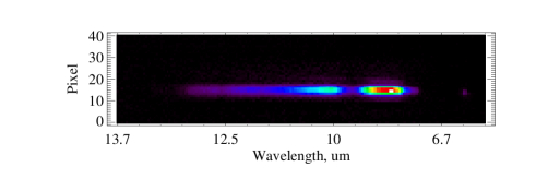
Figure 2: Total intensity from MIDI observations. Left: Coadded intensity frames from an observation of a standard star in a single optical train (in this case HD61935 run D1 beam “A” = telescope UT3). The spectral dispersion runs along the horizontal direction (increasing wavelength from right to left). Right: A cut through one of the spectral channels (at 8.5$\mu$m). This shows the profile of the total intensity along the pixel direction. Overplotted are the EWS default mask (fixed based on observation set-up) and the MIA mask (determined from the intensity image itself). It is evident that the MIA mask fits not only the width of the true detected profile but also the location of the peak on the array much more accurately than the default mask.

The first step in the data reduction involved compressing the fringe and total intensity frames in the direction perpendicular to the spectral dispersion to obtain one-dimensional fringe and intensity spectra. Prior to compression, each frame was multiplied by a mask to reduce the impact of noise. We found that the default EWS masks provided for HIGH-SENS mode observing gave a poor fit to the peak of the detected emission and were much broader than the emission in the direction perpendicular to the spectral dispersion. We therefore used masks determined by a fit to the total intensity frames as provided by the MIA reduction package instead (see Figure 2). We then used the EWS group delay analysis to align the fringes before vector averaging over time to derive the correlated flux (for details see the EWS user manual). The correlated flux $I_{\rm{corr}}$ was then compared to the total source flux, $I_{\rm{tot}}$, to give the source visibility $V=I_{\rm{corr}}/I_{\rm{tot}}$.

2.3 Total Source Intensity

Total intensity data were obtained with MIDI after the fringe observations had been secured as described in Sec. 2.1. The results showed a great degree of variation between different observations of the same object, primarily because of background which could not be perfectly subtracted. We found the background did not vary linearly in the direction perpendicular to the spectrally-dispersed direction, and moreover varied with time during the observations, suggesting that sky (and/or telescope) variations were significant. As the total intensity measurements of the same science target could vary by $>$50%, we chose to use available IRS spectra of our science targets as the total intensity measurements instead. The IRS spectra (originally presented in Chen et al. 2006 and Beichman et al. 2005) were extracted along a slit of width 3$\aas@@fstack{\prime\prime}$7 or 4$\aas@@fstack{\prime\prime}$7 depending on the spectral resolution. Our MIDI data were secured with a slit width of 0$\aas@@fstack{\prime\prime}$52 and so it was necessary to check whether the Spitzer aperture might have included additional photometric signals not seen by MIDI.

For both sources we found there were no background or companion objects in the Spitzer aperture that might be excluded by the MIDI aperture (Smith et al. 2008). The 3 Neptune mass planets discovered within 1AU of HD69830 (Lovis et al. 2006) are not expected to be brighter in the mid-infrared than 10${}^{-3}F_{\star}$ (Burrows et al. 2004), and so would only contribute a discrepancy of at most $\sim$1mJy at 10$\mu$m to our total intensity measurement. A full analysis of the IRS spectra (Lisse et al. 2007) revealed evidence for water ices which, due to their lower temperatures, may reside at larger radial offsets from the star than the bulk of the emission around HD69830. However, as pointed out by the authors the local thermal equilibrium temperature for the region of their best fitting model — a disc at $\sim$ 1AU — is only 245K, cool enough that should the water ice be isolated from the hotter dust particles it could be stabilised by evaporative sublimation. In addition a wide Kuiper belt-like location is ruled out by the 70$\mu$m limits on the excess (1$\pm$3mJy, Beichman et al. 2005). The contribution of the water ice in the 8-13$\mu$m region of the spectrum is at the level of 1-3% of the excess emission between 8-11$\mu$m, rising to 27% of the excess emission at 13 $\mu$m. Thus we believe the effect of the water ice contribution falling outside the MIDI beam can only have a significant effect on the measured flux longwards of 11.5$\mu$m, if at all. The temperature of the dust around $\eta$ Corvi is predicted by SED fitting to be at around 320K, suggesting a small radial offset from the star. The alternative fit to the SED suggested by Chen et al. (2006) suggests there may be dust at two temperatures of 360K and 120K, but the 8–13$\mu$m range is dominated in this model by amorphous olivines at the hotter temperature. Thus in either the single temperature fit or the fit proposed by Chen et al. (2006) the excess emission in the MIDI wavelength range is expected to be dominated by grains close to the star. Therefore for both science targets it is unlikely that significant emission appears in the IRS spectra that would be excluded from our MIDI observations.

2.4 Visibility calibration

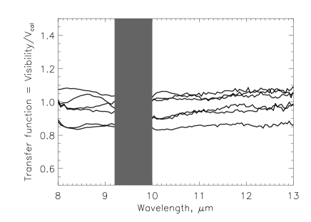
Figure 3: Plots of visibilities determined for standard star targets using other standard stars. Pairs of standard stars observed closely in time were considered as these are the pairings used for science observation calibration. Note that the shaded region 9.2–10$\mu$m is prone to strong uncertainty due to ozone absorption, and so should be ignored. For each pair the ’target’ and ’calibrator’ were chosen randomly. Left: The calibrator-calibrator determined visibilities divided by the predicted visibility for the target star. Perfectly calibrated data would give a straight line at unity with no variation with wavelength. We used the weighted mean (over wavelength) for each calibrator-calibrator dataset to quantify the quality of the calibration and found a range between 0.86 and 1.12. Right: Checking the absolute variation with wavelength for calibrator-calibrator visibilities. All visibilities were scaled to 1 in the range 8–9$\mu$m. The ratio of visibility between 10–11.5$\mu$m and 8–9$\mu$m was calculated to determine the variation of visibility with wavelength. The maximum deviation from unity for this value was 0.047, with some calibrations providing a much flatter visibility.

The total source intensities of the standards, which were chosen for their lack of infrared spectral features as well as their small angular size, were modelled by Rayleigh-Jeans functions scaled to the 10.5$\mu$m flux listed in the spectro-photometric catalogue (see Table 1). The visibilities of the standard stars were calculated assuming these could be modelled as uniform discs with diameters as listed in Table 1.

The calibration of the correlated flux and determination of visibilities for each observation were determined as

$$F_{\rm{corr,tar}}=I_{\rm{corr,tar}}/I_{\rm{corr,cal}}\times F_{\rm{tot,cal}}\times V_{\rm{cal}},$$ (1)

where $I_{\rm{corr,tar}}$ and $I_{\rm{corr,cal}}$ are the correlated fluxes in ADU (output of data reduction procedure) of the target and standard star used as a calibrator respectively, $F_{\rm{corr,tar}}$ is the calibrated correlated flux of the target, $F_{\rm{tot,cal}}$ is the known flux of the standard star (from Rayleigh-Jeans slope) and $V_{\rm{cal}}$ is the visibility of the standard star which is dependent on the baseline length and wavelength. The visibility of the target is then

$$V=F_{\rm{corr,tar}}/F_{\rm{tot,tar}},$$ (2)

($F_{\rm{tot,tar}}$ again from Rayleigh-Jeans slope). For the case of the science targets $F_{\rm{tot,tar}}$ was given by the IRS spectrum. We used the average of the two standards bracketing each science observation to determine the calibrated visibilities, and difference between the two to determine our absolute calibration uncertainties.

We also performed the above calibrations with the standard star observations as “dummy targets” to: 1) determine the level of accuracy to which we could trust the absolute visibility measurements; and 2) examine the visibility functions for evidence of changing visibility with wavelength. Examples of the transfer function of standard – standard calibration (where the standards were observed close in time and space to each other) are given in Figure 3. In the left panel we show the transfer function; the visibility determined for our “dummy targets” as a function of the visibility predicted for this target ($V_{\rm{cal}}$ in equation 1). The absolute levels of this transfer function were found to have a mean and standard deviation of 0.99 $\pm$0.10 (Figure 3 left) after calculating the weighted mean of each visibility over the 8-13$\mu$m range (excluding the 9.2–10$\mu$m region which is dominated by ozone emission). The weights were determined by splitting the fringe data into 5 equal length sets and calculating the variance between these subsets of data at every spectral channel. This absolute variation is the same as the 10% error typically expected in calibration due to changing conditions between observations (e.g. Chesneau 2007). The visibility functions were fairly flat, as shown in the right-hand panel of Figure 3. The weighted mean of each visibility function between 8-9$\mu$m was used to scale the visibilities to 1 in the 8–9$\mu$m range for this plot. The weighted mean for each function between 10–11.5$\mu$m and 8–9$\mu$m were then compared. This ratio was found to be have a mean and standard deviation of 0.991 $\pm$ 0.037. Thus the differential visibility (i.e. the visibility as referenced to that at some fixed wavelength) is typically known with $\sim$ 3 times better accuracy than the absolute visibilities.

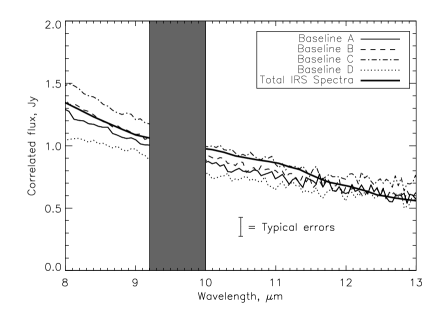
Figure 4: The results of MIDI observations of HD69830. Top left: The baselines observed in this program. Top right: The calibrated correlated fluxes found in the MIDI observations of HD69830. The thick line represents the total IRS spectra, which represents the maximum flux we should see. Note that although the absolute values are varying by $\sim$ 10%, all runs show a fairly flat spectrum, with no evidence of the silicate features seen in the IRS spectra. Bottom left: The visibility of HD69830. The measured visibilities on all four baselines are calculated using the IRS spectra and the measured correlated fluxes. The prediction for what the visibility curve should look like if the disc flux is totally resolved ($V_{\rm{res}}$, equation 4) is also shown by a thick solid line. Bottom right: The visibility of HD69830 scaled to an average of 1 between 8-9 $\mu$m. Notice the shape across all baselines is similar to the $V_{\rm{res}}$ prediction.

3 MIDI results

We now present the results for each of the science targets in turn. To help interpret our results, we consider how the visibility function of a source is expected to behave if the source is made up of multiple components. HD69830 and $\eta$ Corvi have significant stellar emission in the N band (see Table 1). Thus there will be two components to the visibility function, the component from the stellar emission (where the visibility $V_{\star}=1$ as the predicted angular sizes of the stars are 0.63mas for HD69830 and 0.73mas for $\eta$ Corvi based on typical radii for their spectral types and their distances determined by parallax) and the component from the disc (where the $V_{\rm{disc}}$ will depend on the resolution of the disc flux). The total visibility of a star + disc source will then be given by

$$\qquad V_{\rm{tot}}=\frac{F_{\star}}{F_{\rm{tot}}}V_{\star}+\frac{F_{\rm{disc}}}{F_{\rm{tot}}}V_{\rm{disc}},$$ (3)

(where $F_{\star}$ is the flux of the star, etc.). As only the disc components of our targets have the potential to be resolved on the baselines used in this study the equation above predicts a visibility function comprising the sum of two terms. The first of these will vary solely on the ratio of stellar to total flux whereas the second will depend both on the ratio of disc to total flux and on whether the disc is resolved by the interferometric baseline. More precisely, the visibility function will tend to the value of

$$V_{\rm{tot}}\qquad{\longrightarrow\atop V_{\rm{disc\rightarrow 0}}}\qquad V_{\rm{res}}=\frac{F_{\star}}{F_{\rm{tot}}}$$ (4)

when the disc is fully resolved. As can be seen in Figure 1 the value of $V_{\rm{res}}=\frac{F_{\star}}{F_{\rm{tot}}}$ is expected to change across the spectral range of MIDI, particularly in respect of the silicate features seen in the excess emission around both stars. As a result, any variation in observed visibility as a function of wavelength will need to be corrected for this behaviour before it can be interpreted in terms of any resolved source structure.

3.1 HD69830

HD69830 was observed on all four baseline combinations used for this study. A sketch of the geometry of the baselines and relative lengths is shown in Figure 4 (top left).

The calibrated correlated flux for all four baseline observations of this source are shown in Figure 4 (top right). The error bar indicates an average error measured across all four baselines. These errors are determined from two sources: splitting the fringe tracking files into 5 equal subsets and performing the reduction on each subset in turn to determine the variation in fringe signal across the time of the observation (statistical error); and the variation between correlated flux measurements as calibrated by different standard star observations where available. The two sources were added in quadrature. The error is dominated by calibration error which is typically $\sim$10% of the correlated flux (see also 2.4).

The correlated fluxes show variation across the different baselines, as can be seen in the levels of flux measured at 8 $\mu$m. When correlated fluxes are different on different baselines there is the possibility that these differences represent real differences in the resolution of the source. However, at 8 $\mu$m the disc emission is expected to be very low (4 mJy at 8$\mu$m), and so $\sim$ 100% of the emission at $8\mu$m should come from the stellar photosphere. As the star is expected to be point-like and completely unresolved, the correlated flux should equal the total flux (marked by a thick solid line) at this wavelength. The differences in these absolute values are at the expected level of variation in absolute correlated flux from changing conditions between science and standard star observations (see section 2.4).

What is clear from Figure 4 (top right) is that for all baselines the correlated flux is flatter than the total flux measured in the IRS spectrum; there is no evidence of the silicate feature seen between 10–11.5 $\mu$m in Figure 1. As shown by equation 4, if the disc flux is totally resolved ($V_{\rm{res}}$) the correlated flux should consist solely of the stellar photospheric emission - with no evidence of the silicate features seen in the excess emission spectrum. The indication that the disc flux has been at least partially resolved on all baselines is made clearer by examination of the visibility function shown in Figure 4 (bottom left).

The absolute values of visibility across all baselines are an average of 1.04$\pm$0.16. That this variation is a reflection of absolute uncertainty and not evidence of different levels of resolution is confirmed by the visibility at 8 $\mu$m, which as discussed above should be 1 as the flux here is completely dominated by the stellar photosphere. Uncertainty at this level is to be expected, given typical uncertainties in calibrated visibilities of 0.10 (see Figure 3) and the relative faintness of the target (total flux of $\sim$1 Jy across the MIDI spectral range, see Figure 1). Beyond this uncertainty in absolute values, however, the visibilities measured on all four baselines can be seen to dip exactly in the regions we would expect a dip if the disc flux was resolved. This dip is made clearer if we scale the visibility function to 1 averaged over the short wavelength region (8–9$\mu$m), as would be expected even in the resolved disc case ($V_{\rm{res}}$) because of the lack of excess in this region.

Baseline	Visibility
name	8-9$\mu$m	10-11.5$\mu$m	Ratio
A	0.944 $\pm$ 0.003	0.879 $\pm$ 0.005	0.931 $\pm$ 0.037
B	1.003 $\pm$ 0.003	0.928 $\pm$ 0.004	0.926 $\pm$ 0.027
C	1.093 $\pm$ 0.003	1.018 $\pm$ 0.004	0.931 $\pm$ 0.028
D	0.839 $\pm$ 0.006	0.803 $\pm$ 0.005	0.958 $\pm$ 0.039
$V_{\rm{res}}$	0.990	0.860	0.869

Table 3: Measuring the significance of the dip in visibility of HD69830 at 10-11.5 $\mu$m. The values of visibility in each wavelength range are the weighted means taken over all spectral channels in that range, and uncertainties quoted are the standard errors on the weighted mean from statistical uncertainty only (uncertainty in the absolute visibility is higher due to calibration uncertainties). Final error on ratio includes error from the calibrator ratios discussed in section 2.4 and a 1.3% error on the spectral slope of IRS observations (Beichman et al. 2006), as well as the statistical errors from each wavelength range. The $V_{\rm{res}}$ predicted visibility arises from assuming that $V_{\rm{disc}}=0$ (see equation 4).

The scaled visibility functions measured on the four baselines are shown in Figure 4 bottom right. The dip in visibility between 10-11.5 $\mu$m is now very obvious. To confirm the significance of this dip, the unscaled average visibility within the 14 spectral channels between 8-9 $\mu$m was compared to that in the 29 spectral channels between 10-11.5$\mu$m (i.e., around the lowest predicted visibility when $V_{\rm{disc}}=0$). Table 3 presents these weighted means (the weights were determined from the statistical variation within the 5 sub-integrations available for each spectral channel) together with their standard errors. Calibration uncertainty is not included in these values. The visibility ratios presented in the table are the ratio of these weighted means, where we have included a contribution from calibration errors in quadrature with the statistical errors in the 2nd and 3rd columns when evaluating the errors in the final column. These calibration errors arise from two sources. First, as we have used the IRS spectrum to determine the visibilities, we included an error of 1.3% typical of errors on the IRS spectral slope as measured for sources with no observed excess emission (Beichman et al. 2006). Second, we included the error on the ratio from calibration as measured in the standard–standard calibrated visibilities discussed in section 2.4. We used the standard deviation of the visibility ratio (3.7%, section 2.4), but for runs B and C where 2 standard star observations were available for calibration, this was reduced by a factor of $\sqrt{2}$.

For all four baselines used to observe HD69830 the visibility ratio suggests a partial resolution of the disc - the ratio is higher than the 0.869 expected for $V_{\rm{res}}$ but definitely lower than unity. On baselines B and C this difference from unity is significant at a level of $\sim$ 3$\sigma$. When averaged over all 4 baselines the weighted mean of the visibility ratio is 0.934 $\pm$ 0.015. Taken as a whole, these data suggest that the observed visibility ratio is different from 1 at a level of 4$\sigma$. We note in passing that the actual scatter between the four measurements of the visibility ratio is very small, suggesting that we have been conservative in associating an error of $0.015$ to our final “best-estimate”.

We do note, however, that the lower right panel of Figure 4 also shows the visibility function of HD69830 rising beyond $\sim$12$\mu$m to above 1 in the scaled case, meaning the ratios between the weighted mean visibilities between 11.5–13$\mu$m and between 8–9$\mu$m are on average greater than 1 (baseline A 1.045, B 0.991, C 1.043 and D 1.098). For baseline D this ratio is larger than would be expected from any calibration error, as the error on the ratios over the same wavelength ranges from the calibrator-calibrator visibilities (section 2.4) is a maximum of 0.053. The $V_{\rm{res}}$ prediction shows that the visibility function in the case that the disc is completely resolved would be expected to rise, but visibilities should not ever be greater than 1 (see equation 4). This is unlikely to be due to the water ice discussed in section 2.3, as if some of the excess emission measured in the IRS spectrum did fall outside of the MIDI beam we would be over-estimating $I_{\rm{tot}}$ in our calibration, and this would lead to a falsely low visibility. We consider that the lower signal-to-noise in the MIDI fringe measurements on this target at longer wavelengths (signal-to-noise is an average of $\sim$70 between 8–9$\mu$m, 37 between 10–11.5$\mu$m and 15 beyond 12$\mu$m) is the cause of these high visibilities which causes a residual slope. Whether this affects the 10–11.5$\mu$m region is not clear but for this reason we do not consider that the results provide strong evidence for a partially resolved rather than completely resolved disc. The limits we can place on the morphology of the HD69830 debris disc with the results presented in this section are discussed in section 5.1.

3.2 $\eta$ Corvi

$\eta$ Corvi was observed on baselines A and B and on baseline D twice (see Figure 5, top left panel). The second observation on baseline D was carried out with an increased chop frequency and integration time which led to greatly improved intensity calibration data.

The calibrated correlated fluxes for all baselines are shown in Figure 5, top right, where we have included calibration errors and the variation across sub-exposures added in quadrature. The error bar shown is indicative of the average error observed over all baselines. Overplotted on these figures is the total IRS photometry presented in Chen et al. (2006), as also shown in Figure 1.

The correlated fluxes are very similar in shape across all four observations. The absolute values vary by the typical $\sim$10% we expect for absolute variation in correlated flux (see section 2.4), but all show a spectrum consistent with photospheric emission in the Rayleigh-Jeans regime. In common with the result of HD69830, there is no evidence of the spectral feature seen in the IRS total spectrum in any of the correlated flux measurements. This indicates that for this source the disc emission also appears to be partially resolved. Again, the result is made clearer by examination of the visibility function.

The calibrated visibilities for all observations of $\eta$ Corvi are shown in Figure 5 (bottom left), along with the visibility predicted for a completely resolved disc component marked in a thick solid line ($V_{\rm{res}}$, see equation 4). The dip in visibility at $\sim$11.5 $\mu$m is seen very clearly on all observed baselines. Again, as expected, the variations between different baselines in terms of absolute values are an average of $\sim$0.1, with a maximum difference of $\sim$0.2. The visibilities scaled to the $V_{\rm{res}}$ prediction between 8–9$\mu$m are shown in Figure 5 (bottom right). Although we do not know what the visibility should be at 8–9$\mu$m for $\eta$ Corvi (as we do for HD69830) as there is significant disc flux in this range, this scaling allows the shape of the visibility function to be seen more clearly and allows easy comparison with the $V_{\rm{res}}$ model.

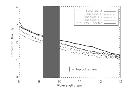
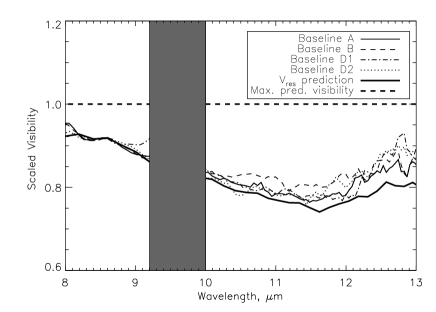
Figure 5: The results of MIDI observations of $\eta$ Corvi. Top left: The baselines observed in this program. Top right: The calibrated correlated fluxes found in the MIDI observations of $\eta$ Corvi. The thick line represents the total IRS spectra, which represents the maximum flux we should see. Note that although the absolute values are varying by $\sim$ 10%, all runs show a fairly flat spectrum, with no evidence of the silicate features seen in the IRS spectra. Bottom left: The visibility of $\eta$ Corvi. The measured visibilities on all four baselines are calculated using the IRS spectra and the measured correlated fluxes. The prediction for what the visibility curve should look like if the disc flux is totally resolved ($V_{\rm{res}}$, equation 4) is also shown by a thick solid line. Bottom right: The visibility of $\eta$ Corvi scaled to the average visibility from the $V_{\rm{res}}$ prediction between 8-9 $\mu$m. This scaling shows the four observations all show strong evidence of being similar to the $V_{\rm{res}}$ prediction.

In Table 4 the weighted mean visibilities in the short wavelength region (8–9 $\mu$m) and the region in which the silicate excess feature has the strongest contribution to the total flux (10–11.5 $\mu$m) are listed. Standard errors and errors on the ratio including calibration uncertainty are calculated as described for HD69830 in section 3.1. As is clear from the table the difference seen in the measured visibilities at shorter wavelengths and midway through the MIDI range (10-11.5$\mu$m) is significant. Not only this, but the size of the change is similar in all cases to that predicted for the case of completely resolved excess emission, as can be seen in the scaled visibility function plots (Figure 5 bottom right). Results on individual baselines are incompatible with an unresolved disc (ratio = 1) at a level of at least 4 $\sigma$ (see Table 4). Taking all the results together (see footnote 1) the weighted mean dip in visibility is 0.880 $\pm$ 0.013, incompatible with an unresolved disc at the $9\sigma$ level. The individual measured ratios and average result are close to the prediction for a completely resolved disc ($V_{\rm{res}}$). Note that we do not see the same evidence for a significant residual slope in the visibility function as was the case for HD69830. The observations of $\eta$ Corvi benefit from a higher signal-to-noise even at longer wavelengths (average signal-to-noise in the correlated flux measurements is 128 at 8–9$\mu$m, 75 at 10–11.5$\mu$m and 31 at wavelengths beyond 12$\mu$m). Though the levels of absolute calibrated flux and thus visibility are not constrained to better than 10%, (see section 2.4) the dip and its appearance at a significant level across all baselines is consistent with the disc emission being completely resolved on all observed baselines. The constraints we can place on the morphology of this source based on these results are discussed in section 5.2.

Baseline	Visibility
name	8-9$\mu$m	10-11.5$\mu$m	Ratio
A	1.016 $\pm$ 0.005	0.892 $\pm$ 0.004	0.877 $\pm$ 0.026
B	0.910 $\pm$ 0.003	0.818 $\pm$ 0.003	0.899 $\pm$ 0.027
D1	0.841 $\pm$ 0.003	0.739 $\pm$ 0.003	0.879 $\pm$ 0.026
D2	0.922 $\pm$ 0.003	0.801 $\pm$ 0.004	0.868 $\pm$ 0.026
$V_{\rm{res}}$	0.915	0.784	0.857

Table 4: Measuring the significance of the dip in visibility of $\eta$ Corvi at 10-11.5 $\mu$m. A description of the calculation of the visiblities and errors is given in the caption to Table 3.

4 VISIR imaging of HD69830

Standard

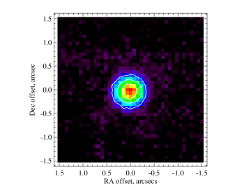
HD69830

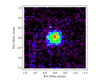
Residuals

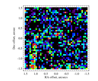
Figure 6: The VISIR images of HD69830 and standard star observed in filter Q2. Left: The final image of standard star (HD61935) after co-addition of 4 sub-integrations. This image acts as a PSF reference. Middle: The final image of HD69830. Contours on this and the standard star are at levels of 25, 50 and 75% of the peaks. No evidence of emission extended beyond the PSF reference is seen in the image of HD69830. The colour scale on these images goes from 0 to the peak. Right: The image of HD69830 after subtraction of the PSF reference (standard image) scaled to the peak. The colour scale has a minimum of 0 and maximum of 3$\sigma$ per pixel. Contours mark any region of $>$2sigma significance. The stripe to the South East of the image is a detector artifact. No significant emission is seen after subtraction of the PSF which would indicate resolved emission (testing over a range of regions of different shapes which could detect a range of different disc geometries gives a maximum detection of $<$2$\sigma$ in this image).

Following the 8m limits on the $\eta$ Corvi emission presented in Smith et al. (2008), we have new data obtained on VISIR at the VLT under proposal 079.C-0259 on 6^th April 2007 on the emission around HD69830. The data were all taken in filter Q2 ($\lambda_{c}=18.72\mu$m, $\Delta\lambda=0.88\mu$m) with pixel scale 0$\aas@@fstack{\prime\prime}$075. The observations were performed using a chop and nod throw of 8″. Chopping was performed in a North-South direction and nodding was performed in the perpendicular direction. The observations consisted of two integrations of 2100s each on HD69830, with standard star observations before and after each science target integration (125s per integration). Frequent standard star observation was used to determine how the PSF was varying through the observations. The standard star observations were also used for photometric calibration. The standard star, HD61935, was chosen from a list of mid-infrared spectro-photometric standards (Cohen et al. 1999) and was also used in the MIDI observations (Table 1). The observations are summarised in Table 5.

The data were reduced using custom routines described in detail in Smith et al. (2008). In summary, data reduction involved determination of a gain map using the mean values of each frame to determine pixel responsivity (masking off pixels on which emission from the source could fall, equivalent to a sky flat). In addition a dc-offset was determined by calculating the mean pixel values in columns and rows (excluding pixels on which source emission was detected) and this was subtracted from the final image to ensure a flat background. Pixels showing high or low gain, or those which showed great variation throughout the observation, were masked off. The chop-and-nod pattern adopted results in four images of the star falling on the detector. These images were co-added after determining the centre of each image by 2-dimensional Gaussian fitting and then the sub-integrations were added together to give a final image of HD69830 and the standard star which would act as a PSF reference.

Target	Target type	Integration time (s)
HD61935	Cal	125
HD69830	Sci	2100
HD61935	Cal	125
HD61935	Cal	125
HD69830	Sci	2100
HD61935	Cal	125

Table 5: The observations of HD69830 and standard star with VISIR on the VLT. Observations were performed under proposal 079.C-0259. All observations were performed using filter Q2 and the small field detector (pixel scale 0$\aas@@fstack{\prime\prime}$075).

The photometry was performed using circular apertures of 1″radius centred on the peak of the emission. Statistical background noise was calculated in annuli centred on the peak of emission with inner radius 2″, outer radius 4″. Calibration uncertainty was estimated from the variation in calibration levels from the four sub-integrations on the standard star, and was found to be 9%. HD69830 was detected in the final co-added image with a signal-to-noise of 32, with the total photometry including calibration uncertainty of 377 $\pm$ 46 mJy. The IRS spectrum of this source has a flux of 365 mJy at 18.72$\mu$m (253 mJy expected from the photosphere). No colour-correction was applied for this narrow-band filter. In addition, no correction for airmass was employed, as the standard star was observed at a similar airmass to HD69830 and no evidence was found that the calibration factors from the sub-integrations on the standard star were correlated with airmass.

The final images of the standard star HD61935, used as a PSF reference, and of HD69830 are shown in Figure 6. Overplotted on the images are contours at 25, 50 and 75% of the image peak (brightness peaks were 7980 mJy/arcsec² for the standard star observation, 1033 mJy/arcsec² for HD69830). Comparison of the contour plots indicates that there is no sign of extended emission around HD69830 that could be indicative of a resolved disc. This is confirmed by examination of the residuals image (Figure 6 right). This is the HD69830 image after subtraction of the PSF reference image (HD61935, Figure 6 left) scaled to the peak of emission. The residual image shows no evidence for emission beyond the PSF. Further tests comparing the profiles of the observations, Gaussian and Moffat profile fits to the images and comparisons of FWHM measurements all confirmed this result. Different test regions (annuli of different dimensions for face-on disc geometries, rectangular boxes for edge-on discs, and intermediate shapes for discs with intermediate inclinations to the line of sight) were also examined for any evidence of significant emission in the residuals image. No such emission was found (most significant positive flux of just less than 2$\sigma$ significance was found in a region including a detector artifact - see Figure 6).

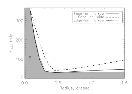
Figure 7: The limits we can place on the geometry of the HD69830 following no detection of extended emission in the VISIR Q band imaging. Discs in the space above the lines should have been detected in our imaging, and those lying in the shaded region would have remained undetected regardless of geometry. Different lines represent different disc geometries as given in the legend. Narrow discs have a disc width of $0.2r$, wide discs a width of $2.0r$, where $r$ is the radius of the mid-point of the disc. The expected disc flux and location from the SED is marked by an asterisk, with error bars representing the uncertainty in $R_{\lambda}$ from errors in the IRS spectrum.

We followed the procedure of Smith et al. (2008) to place limits on the size of the disc after no extension was detected. This procedure is described in detail in Smith et al. (2008), and involves convolving the PSF model with different disc + star models to determine what combinations of disc parameters (geometry and emission level) would have resulted in a detection of extended emission. The limits depend strongly on the sensitivity of the observation and the variation of the PSF, which was determined in this case from examination of the four sub-integrations on the standard star. The PSF was found to have a FWHM of 0$\aas@@fstack{\prime\prime}$52$\pm$0.04, a variation of 7%. The individual integrations gave four separate PSF models which were used in the limits testing, with variations between the results being the limiting factor on disc detection at small disc radii. The results of this testing are shown in Figure 7. For a face-on disc assuming a narrow ring-like structure (width $0.2r$ where $r$ is the disc radius) the extension testing places a limit of $<$0$\aas@@fstack{\prime\prime}$19 $\pm$ 0$\aas@@fstack{\prime\prime}$01 on the disc radius ($<$2.4 AU at a distance of 12.6pc). This limit is determined by the size and variation of the PSF (limiting line at small disc radii is near vertical as it is not strongly dependent on the disc flux). A PSF variation of 7% is fairly typical for Q band observations taken under good conditions based on previous observing experience (see e.g. Smith et al. 2008, 2009). Only observations taken under optimal (very stable seeing) conditions would allow us to probe closer to the star, and then only by perhaps one or at best two tenths of an arcsecond ($\sim$0.1-0.25AU). This limit assumes disc emission is 112$\pm$15mJy (3$\sigma$ limit using errors from IRS photometry), as measured in the IRS spectrum assuming a Kurucz model profile for the photosphere and in agreement with our photometry. Limits on broader discs arise from the sensitivity of the observations, and could be improved with increased observation time. With the current limits, we can rule out any disc brighter than 33mJy at a radius of 0$\aas@@fstack{\prime\prime}$5 (6.3AU) with some dependence on the assumed disc geometry (Figure 7).

5 Discussion

We now consider the implications for the geometries of the HD69830 and $\eta$ Corvi discs in the mid-infrared following the MIDI results and the constraints from 8m imaging.

5.1 HD69830

The MIDI correlated fluxes measured for HD69830 and the visibility functions determined from these are consistent with the detection of photospheric emission only. The slopes are consistent with a Rayleigh-Jeans slope, and there is no evidence of the silicate feature observed in the IRS spectrum. We thus conclude that the excess emission does not strongly contribute to the correlated flux and therefore this has been at least partially resolved on the observed baselines.

Evidence for resolved emission around $\zeta$ Aql in the near-infrared was interpreted as evidence for a low-mass companion object (Absil et al. 2008). We do not believe this is the explanation for the resolved emission around HD69830, since the emission spectrum is consistent with dust emission (Beichman et al. 2005; Lisse et al. 2007), and the observed visibility ratio is the same (within the errors) on all observed baselines. The same resolution on near perpendicular baselines such as A and B/D (see Table 2 and Figure 4 top left) would not be expected if the emission arose from a point-like source. Furthermore extensive radial velocity observations have revealed only low-mass companions (Lovis et al. 2006) orbiting within 1AU, believed to be Neptune-mass (although the masses could be larger if the system is observed face-on). Such planets cannot be the source of the observed change in visibility with wavelength due to the low expected star:planet mid-infrared flux contrast of $<10^{-3}$ (see e.g Burrows 2005; Burrows et al. 2006).

The observed visibilities are consistent with a partial resolution of dust emission around HD69830. Assuming that the stellar component has a visibility of 1, and that the values of $F_{\star}$ and $F_{\rm{disc}}$ are accurately given by a Kurucz model profile and the IRS spectra from Beichman et al. (2005), the visibility ratios listed in Table 3 can be used to estimate the disc location given certain assumptions about the morphology of the emission. For example, assuming that the disc emission has a Gaussian distribution gives a best fit FWHM of 10mas. As many debris discs resolved to date have been found to have ring-like structure (see, e.g. Greaves et al. 2005; Kalas et al. 2005; Schneider et al. 2009), we also modelled the observed visibilities assuming the disc emission to originate in symmetric, face-on rings with varying radii and widths of $dr/r=0.2,1$ or 2 where $r$ is the radius of the middle of the ring (see appendix A). Figure 8 shows the results of a $\chi^{2}$-test of the goodness-of-fit of each model suggesting a best-fit disc radius of 10–25mas, depending on the width of the ring. Both tested morphologies predict a best-fit radius of 0.1-0.3AU at 12.6pc which would place the dust in the middle of the planetary system. A stability analysis by Lovis et al. (2006) used Monte-Carlo modelling to determine locations where massless particles could have long-term stable orbits in the presence of the 3 Neptune-mass planets, finding 2 long-term stable zones at 0.3–0.5AU and $>$0.8AU. Thus the visibilities suggest a best-fit location for the dust compatible with the inner stable zone.

Figure 8: The limits on the HD69830 disc from the MIDI observations. Left: The confidence limits found comparing the observed visibility ratios on all 4 baselines with those predicted by face-on ring-like models for the disc morphology (of radius $r$ and width $dr$). Lower values of $\chi^{2}$ represent a better fit to the data, and the horizontal dotted lines denote the level at which the models are consistent with the observations at the 1, 2 and 3$\sigma$ levels as determined by the percentage points of the $\chi^{2}$ distribution function with 4 degrees of freedom. The limits depend on the assumed width of the ring as indicated in the legend. Right: Predicted visibility ratios for narrow ($dr/r=0.2$) ring-like models of radii 5, 10, 25 and 80mas (solid lines). The ratio expected if the disc emission is completely resolved (i.e., the $V_{\rm{res}}$ prediction) is shown by a dashed line. Observed visibility ratios are shown with asterisks and 1$\sigma$ error bars (Table 3). The modest level of significance with which different models fit the observations (seen in the left figure) is due to the complex visibility function for ring models, combined with sparse baseline coverage and large uncertainties. See Appendix A for details of modelling and error calculations.

However, uncertainties in the visibility ratios mean that the observations are also consistent within the uncertainties with a bigger radial location (see Figure 8), particularly if the possible slope on the visibilities is taken into account (see section 3.1). Should the high levels of visibility seen at long wavelengths be evidence of a residual slope, then the disc emission may be completely resolved on these baselines (in which case the visibility would match the $V_{\rm{res}}$ prediction). For this to be the case we would require a Gaussian of FWHM $>$ 22mas (0.28AU) on an average baseline of 83m, or of at least 40mas (0.5AU) to be completely resolved on baseline B (44m). These sizes are consistent both with the inner stable zone of Lovis et al. (2006), and a larger radial location outside the orbits of the planets. A larger radial location is favoured from analysis of the IRS spectrum which suggests the emission originates in disrupted P or D-type asteroids at a distance of 0.9–1.1AU (Lisse et al. 2007). If there is not a residual slope on the data, and the results are truly indicative of a partial disc resolution, the dust would then be constrained to lie within the orbits of the planets challenging current SED models.

Regardless of the residual slope, the MIDI observations are inconsistent with unresolved emission, and so limits can be placed on the minimum radius of the dust emission. Using ring-like models we find a 3$\sigma$ limit on the radius of $>$4mas (0.05AU), or from Gaussian models we find a 3$\sigma$ limit on the FWHM of $>$4mas. The VISIR data (section 4) provides a complimentary upper limit on the disc radius of $<$2.4AU.

Adopting the radial size of 1AU from the SED modelling, we compared the observations to model predictions for 1AU rings inclined both edge-on, face-on and 45^∘ to the line-of-sight and at different position angles to assess whether the observations show evidence for an inclined disc structure; measurement of the disc inclination would remove ambiguity in the planet masses assuming these were orbiting in the same plane. A narrow edge-on disc lying at a position angle of $\sim$165^∘ provides the best fit to the four observed visibility ratios ($\chi^{2}$ minimum of 1.3$\sigma$, Figure 9; other disc widths provide worse fits to the data, albeit still within observational uncertainties). Inclined discs at other position angles away from $\sim$60^∘ also provide better fits to the data than a face-on model, although a narrow face-on disc at 80mas is consistent with the observed visibilities at a level of 3$\sigma$. Thus with the current data we cannot place significant limits on the disc inclination. The lack of significant differences in the visibility ratios on different baselines also means there is no evidence for clumpy and asymmetric structure, although the uncertainties in the data mean that such structure cannot be ruled out.

Figure 9: Comparison of inclined disc models to the observed visibility ratios of HD69830 at a fixed disc radius of 80mas. Inclinations are measured from face-on = 0^∘.

Taking the stability analysis of Lovis et al. (2006) and the SED modelling of Lisse et al. (2007) together with the MIDI and VISIR results presented here, we consider the emission from this system to be most likely smooth and symmetric at $\sim$1AU radius.

5.2 $\eta$ Corvi

Figure 10: The limits on the $\eta$ Corvi warm dust from the MIDI observations. Left: The confidence limits found comparing the observed visibility ratios on all 4 baselines with those predicted by face-on ring-like models for the disc morphology (of radius $r$ and width $dr$). Lower values of $\chi^{2}$ represent a better fit to the data, and the horizontal dotted lines denote the level at which the models are consistent with the observations at the 1, 2 and 3$\sigma$ levels as determined by the percentage points of the $\chi^{2}$ distribution function with 4 degrees of freedom. The limits depend on the assumed width of the ring as indicated in the legend. Right: Predicted visibility ratios for narrow ($dr/r=0.2$) ring-like models of radii 5, 10, 25 and 90mas (solid lines). The ratio expected if the disc emission is completely resolved (i.e., the $V_{\rm{res}}$ prediction) is shown by a dashed line. Observed visibility ratios are shown with asterisks and 1$\sigma$ error bars (Table 4). The modest level of significance with which different models fit the observations (seen in the left figure) is due to the complex visibility function for ring models, combined with sparse baseline coverage and large uncertainties. See Appendix A for details of modelling and error calculations.

The MIDI correlated fluxes are consistent with Rayleigh-Jeans emission across the MIDI range. We see no evidence of the mid-infrared excess emission dominated by silicate emission in the correlated fluxes and conclude that the data are consistent with all of the excess being resolved on the observed baselines. As for HD69830, we rule out a companion object as the source of the resolved emission due to the silicate emission feature seen in the IRS spectrum (Chen et al. 2006) and the lack of a known binary companion. Limits from radial velocity searches rule out a planet of mass $>$0.4$M_{\rm{Jup}}$ with a period of 3 days or less, and a planet of mass $>$2.1$M_{\rm{Jup}}$ with a period of 100 days or less (corresponding to $<$0.46AU for $M_{\star}=1.5M_{\odot}$), at the 3$\sigma$ confidence level (Lagrange et al. 2009).

The observed visibilities are consistent with at least partial, perhaps complete, resolution of the dust emission. The observed visibility ratios were modelled in a similar manner to HD69830. Assuming that the disc emission has a Gaussian distribution results in a best fit FWHM of 27mas. The comparison with ring-like models is shown in Figure 10, from which best-fit disc radii are 20–25mas for wider rings, or $>$50mas for narrow face-on rings ($>$0.91AU). A size of 20-50mas translates to a radius of 0.4-0.9AU at 18.2pc. Since the MIDI observations are inconsistent with unresolved emission, they can be used to derive a minimum size for the emitting region. Assuming a Gaussian distribution for the disc emission limits the FWHM to $>$14mas ($>$0.25AU; 3$\sigma$ limit from $\chi^{2}$ goodness-of-fit over all 4 baselines), whereas the ring-like models constrains the radius to $>$9mas (0.16AU, $3\sigma$ limit).

There remains some uncertainty from SED modelling on the location of the mid-infrared excess, with two models proposed that suggest that either the hot dust lies in a single ring at 1.7AU or in two radial locations at 1.3 and 12AU (Chen et al. 2006). Smith et al. (2008) ruled out the 12AU component at the 2.6$\sigma$ level, since this was not resolved in VISIR 18.7$\mu$m imaging, so that a single ring at 1.7AU remains the best estimate of the radius of the hot dust from the SED, with unresolved 8m imaging constraining the location of a single radius component to $<3$AU. Thus, like HD69830, the best-fit radius is smaller than, but not inconsistent with that predicted from SED modelling (90mas, 1.7AU, Smith et al. 2008); the narrow ring models are most consistent with the SED models, however the errors on the data and the complex visibility functions expected for ring-like structure (Figure 10, right) mean that a large range of ring models provide a good fit to the data within the errors. In contrast to HD69830 no planets are known to be orbiting interior to the dust, although limits are not so stringent (Lagrange et al. 2009).

Adopting a radius of 1.7AU for the dust from SED modelling, we compared the observations to model predictions for 1.7AU rings inclined both edge-on, face-on and at 45^∘ and 70^∘ to the line-of-sight and at different position angles to attempt to constrain the inclination and position angle of such a disc. The best fitting disc geometry was found to be a broad edge-on disc at a position angle of $\sim$120^∘ (Figure 11). For narrow discs all geometries are within 1$\sigma$ of the best fitting model, and for broad discs only edge-on discs with a position angle $\sim$15^∘ are outwith 1$\sigma$ of the best fit. Thus other disc geometries cannot be ruled out with the current data. However, it is notable that this best-fit position angle coincides with that of a cold disc component (at 130$\pm$10^∘) imaged in the sub-mm and inferred to be in a 150$\pm$20AU ring inclined by 45$\pm$25^∘ to our line-of-sight (Wyatt et al. 2005). A common position angle would suggest that both dust components, over two orders of magnitude in radius, originate from planetesimals orbiting in the same plane.

There is no evidence from this data for asymmetric of clumpy structure, since the visibility functions are consistent (within the errors) with the same level of resolution on all baselines (Figure 5). This level is consistent with the excess being completely resolved on all baselines (i.e., it coincides with the $V_{\rm{res}}$ prediction). We note that this does not mean that the emission comes from a region which appears the same size on all observed baselines, but that on each baseline the emission covers a large enough region to have been completely resolved.

Taking the MIDI results and combining them with the results from 8m imaging in Smith et al. (2008) and the IRS spectrum presented in Chen et al. (2006), we consider the emission from this system to be most likely smooth and symmetric at 1.7AU radius, with tentative evidence for extension along a position angle aligned with the cool outer disc.

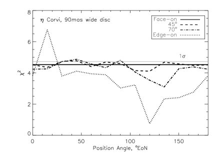
Figure 11: Comparison of inclined disc models to the observed visibility ratios of $\eta$ Corvi at a fixed disc radius of 90mas. Inclinations are measured from face-on = 0^∘.

5.3 Transient sources of emission

For both sources we infer the dust to lie at 1-1.7AU and so consider that it must have a transient origin (Wyatt et al. 2007). One possible source for the transient emission is a recent massive collision within a coincident planetesimal belt (a possibility proposed for BD+20307, see Zuckerman et al. 2008, and references therein). The emission from such an event might be expected to be clumpy or asymmetric as the dust would start off concentrated in a small spatial region (rather than dispersed in a ring like an asteroid belt for example). There is no evidence for such a structure from the MIDI observations. Furthermore this scenario was considered as possible but unlikely due to the expected low frequency of sufficiently massive collisions and the lifetime of resulting dust particles from such events (Wyatt et al. 2007). Thus it seems more likely that the parent bodies of the dust seen at $\sim$1AU originated in a planetesimal belt at larger distances where collisional timescales are much longer. The mechanism transporting the dust into 1AU remains unknown, though one possibility is a dynamical instability in a period analogous to the Late Heavy Bombardment (LHB) in the Solar System (Gomes et al. 2005; Booth et al. 2009), the cause of which could be a recent stellar flyby or the migration of giant planets in the system.

The known cool dust population toward $\eta$ Corvi (Wyatt et al. 2005) could represent the outer parent planetesimal belt suspected to be feeding the hot dust, a suggestion supported by the tentative evidence from the MIDI observations for a position angle for the hot component (120^∘) that is similar to that of the cool dust (130$\pm$10^∘). However, the errors and sparse baseline coverage of the current data do not allow significant limits to be placed at this stage on the hot disc’s inclination and position angle. In contrast no cold dust population has yet been detected around HD69830. Indeed the MIPS photometry limits the excess emission at 70$\mu$m to 1$\pm$3 mJy (Beichman et al. 2005), with SCUBA photometry limiting excess flux at 850$\mu$m to $<$7mJy (Sheret et al. 2004; Matthews et al. 2007), indicating that there is little if any cold dust in the system. One possible way around the conclusion that the dust has to be transient was suggested by Payne et al. (2009), who considered the dynamical evolution of the HD69830 planetesimal disc during the growth and migration its 3 planets (Alibert et al. 2006). In their model significant planetesimal mass remained outside 1AU on high eccentricity orbits, and they suggested that the increased collisional lifetime of highly eccentric orbits could allow significant mass to persist even to 2Gyr, a possibility which is currently being investigated.

6 Conclusions

In this paper we present MIDI observations of HD69830 and $\eta$ Corvi, which for the first time resolve the hot dust emission in these systems, and setting lower limits on the radial location of the emission of $>$0.05AU and $>$0.16AU, respectively. We also present new VISIR observations of HD69830 which show no evidence for resolved emission, thus constraining the radial location of the emission to $<$2.4AU. Similar 8m observations of $\eta$ Corvi were already presented in Smith et al. (2008) showing this emission originates $<$3AU. These mid-infrared observations thus place the dust squarely at a location consistent with that predicted from SED modelling at 1.0 and 1.7AU for HD69830 and $\eta$ Corvi respectively. At such a location the emission to both sources is expected to be transient.

There is no evidence from the MIDI data that the emission is anything but smooth and symmetric. However, assuming a 1.7AU radius for the emission toward $\eta$ Corvi the data marginally favour a more edge-on disc lying at a position angle consistent with that of the known 150AU cool disc at 130$\pm$10^∘. Such a correlation would further support the suggestion that the cool outer disc is feeding the inner disc. The MIDI data also suggest that the HD69830 emission is partially, rather than completely, resolved, placing it at 0.1–0.3AU. Observational uncertainties, including a possible residual slope, mean that this interpretation is not favoured at present given the SED constraints, but if confirmed would present a challenge to the current modelling of the IRS spectra of this source.

These observations highlight the viability of exploration of dust in terrestrial planet regions using mid-infrared interferometry. Future MIDI observations of HD69830 and $\eta$ Corvi that extend the baseline coverage would allow more stringent constraints to be placed on the geometry of these debris discs, including measuring the disc inclination for HD69830 (thus constraining the masses of planet found by radial velocity studies), the disc position angle for $\eta$ Corvi (for comparison with that of the outer cool disc), and searching for the clumpy or asymmetric structure that might be expected from a recent massive collision. Such observations thus have significant potential to constrain the different theories for the origin of these unusual hot dust populations.

Appendix A Modelling the MIDI observations

In this appendix we outline the method used to compare models for geometry of the excess emission to the MIDI data. We consider symmetric Gaussians of varying FWHM and ring models. The ring models are face-on axisymmetric discs with a fixed width and varying radius. The disc is assumed to be centred on the point-like star and has uniform surface brightness. The tested widths are $dr/r=0.2,1$ or 2, with different disc radii, parameterised by $r$, the mid-point of the disc (so disc has inner radius $r-dr/2$, outer radius $r+dr/2$) with $r$ between 5–200 mas. Due to the large range of possible non-axisymmetric disc models (for example discs with brightness asymmetries or clumps, or those inclined to the line of sight at all position angles) we consider only a restricted range of discs outside these face-on models. These were edge-on discs and those inclined at 45 and 70^∘ to the line-of-sight. These discs were assumed to have a fixed radius (80mas for HD69830, 90mas for $\eta$ Corvi; sizes from SED fitting) and had position angles on sky of 0–180^∘ East of North in steps of 15^∘.

The excess region (Gaussian or ring) visibilities were determined using the Interferometric Visibility Calculator available at http://www.mporzio.astro.it/%7Elicausi/IVC/. Determination of the total model visibility then follows from equation 3, assuming the visibility of the star is 1 at all wavelengths. We determined the visibility for the models across the wavelength ranges used in the characterisation of the dips (i.e. 8–9$\mu$m and 10–11.5$\mu$m, Tables 3 and 4). The models assume flux ratios for the star and disc components are accurately given by the IRS photometry and the Kurucz model profiles.

A.1 Applying a goodness-of-fit test

As the absolute levels of visibility are poorly constrained but the ratio of visibilities at different wavelengths is constrained much better (see sections 2.4, 3.1 and 3.2), we shall use comparison between the observed and model visibility ratios to determine the goodness-of-fit of different models. The sources of error for this comparison must be carefully considered to allow an accurate goodness-of-fit calculation.

In this paper we have used the IRS photometry to calculate visibilities. Following equations 1 and 2, each observed visibility is calculated as

$$V=I_{\rm{corr,tar}}/I_{\rm{corr,cal}}\times F_{\rm{tot,cal}}/F_{\rm{tot,tar}}\times V_{\rm{cal}}.$$ (5)

When we consider the ratio of visibilities, we divide the two visibilities as averaged over the appropriate wavelength ranges

$$V_{\rm{obs,ratio}}=\frac{I_{\rm{corr,tar,10}}}{I_{\rm{corr,tar,8}}}\times\frac{F_{\rm{tot,cal,10}}}{F_{\rm{tot,cal,8}}}\times\frac{I_{\rm{corr,cal,8}}}{I_{\rm{corr,cal,10}}}\times\frac{F_{\rm{tot,tar,8}}}{F_{\rm{tot,tar,10}}}\times\frac{V_{\rm{cal,10}}}{V_{\rm{cal,8}}}$$ (6)

where the subscript 10 refers to the value of this term averaged over the wavelength range 10–11.5$\mu$m, and the subscript 8 refers to averaging over the range 8–9$\mu$m. We now consider the errors from each term in the above equation.

The first term in equation 6, $\frac{I_{\rm{corr,tar,10}}}{I_{\rm{corr,tar,8}}}$, is from the correlated fluxes as measured in the fringe tracking. Errors in each wavelength range are given by variation in the five sub-integrations of the fringe tracking (as given in Tables 3 and 4) and are propagated as $\sigma_{I,\rm{ratio}}/I_{\rm{ratio}}=\sqrt{(\sigma_{I,8}/I_{8})^{2}+(\sigma_{I,10}/I_{10})^{2}}.$ The second term, $\frac{F_{\rm{tot,cal,10}}}{F_{\rm{tot,cal,8}}}$, is given by Kurucz model profile fits to the standard stars. As the slope is considered to be well modelled by such profiles in the mid-infrared and there are no spectral features expected in this range for the standards we consider errors on this term to be negligible. The third term, $\frac{I_{\rm{corr,cal,8}}}{I_{\rm{corr,cal,10}}}$, comes from the standard star correlated flux measurements. As shown in section 2.4 this ratio should always be 1 but has an error of 3.7%. In those instances in which an average calibration from two standard star observations was used this error can be reduced by a factor of $\sqrt{2}$. The term $\frac{F_{\rm{tot,tar,8}}}{F_{\rm{tot,tar,10}}}$ is given by the IRS spectrum of each target. For this we must consider how well the IRS spectra captures the shape of a spectrum. Beichman et al. (2006) showed that for Sun-like stars with no excess emission deviations from a photospheric slope were 1.3% in the range 8.5–13$\mu$m after removing the effects of absolute calibration error (by scaling to the photospheric model at 7–8$\mu$m). The stars included in this study are of the same or similar spectral type to HD69830 (which was in fact included in the sample). $\eta$ Corvi was just excluded by spectral type; the paper considered stars in the range F5–K5, but we do not consider an F2 star likely to be very different to this sample. We therefore use the error of 1.3% as the error on the total flux ratio for the science targets. The term $\frac{V_{\rm{cal,10}}}{V_{\rm{cal,8}}}$ is determined by the assumed size of the standard star used for calibration and in these calculations is assumed to be perfect. In fact as can be seen in Table 1 there is an uncertainty on the size of the standard stars. This uncertainty is very small however (typically 0.01mas) and potential error on the calibrator visibility ratio is thus very small ($<$0.01%). We therefore neglect this uncertainty in our error calculations.

To calculate the same ratio for each model we must use the following equation (c.f. equation 3):

$$V_{\rm{mod,ratio}} = \frac{(F_{\star\rm{,tar,10}}/F_{\rm{tot,tar,10}})+(F_{\rm{disc,tar,10}}/F_{\rm{tot,tar,10}})V_{\rm{disc,tar,10}}}{(F_{\star\rm{,tar,8}}/F_{\rm{tot,tar,8}})+(F_{\rm{disc,tar,8}}/F_{\rm{tot,tar,8}})V_{\rm{disc,tar,8}}}$$ (7)

$$= \frac{F_{\star\rm{,tar,10}}}{F_{\star\rm{,tar,8}}}\times\frac{F_{\rm{tot,tar,8}}}{F_{\rm{tot,tar,10}}}\times\frac{1+V_{\rm{disc,tar,10}}\left(\frac{F_{\rm{tot,tar,10}}}{F_{\star\rm{,tar,10}}}-1\right)}{1+V_{\rm{disc,tar,8}}\left(\frac{F_{\rm{tot,tar,8}}}{F_{\star\rm{,tar,8}}}-1\right)}$$

where it has been assumed the $V_{\star}$ is 1 in both wavelength ranges (see section 3). The errors on each term for the model ratio also require careful consideration. The first term in equation 7, $\frac{F_{\star\rm{,tar,10}}}{F_{\star\rm{,tar,8}}}$, comes from Kurucz model profiles, and again as the stellar emission in this range can be considered to have a well-defined slope the error on this term is negligible. The second term, $\frac{F_{\rm{tot,tar,8}}}{F_{\rm{tot,tar,10}}}$, again comes from the IRS spectrum of this source, and thus we again consider the errors on this ratio to be 1.3% (see above).

The errors on the final term in equation 7 are more complex. We consider that for each model the visibility $V_{\rm{disc,tar}}$ is perfectly known. However errors on $F_{\rm{tot,tar}}/F_{\star\rm{,tar}}$ in both wavelength ranges come from a variety of sources, some of which are systematic across the different wavelength ranges considered. In order to determine the error on this factor we used a Monte-Carlo method. For each model (each with a fixed $V_{\rm{disc,tar,8}}$ and $V_{\rm{disc,tar,10}}$ for each baseline) the value of this final factor was calculated over 1000 iterations, with the values of $F_{\rm{tot,tar}}$ and $F_{\star\rm{,tar}}$ chosen as follows. The values of $F_{\star\rm{,tar,8}}$ and $F_{\star\rm{,tar,10}}$ were determined by using the Kurucz model profile for the correct spectral type (see Table 1). Scaling was determined by taking the $\chi^{2}$ minimisation over a range of scalings to find the best fit to the B- and V-band magnitudes of the stars as listed in the Hipparcos catalogue and J-, H- and K-band magnitudes from the 2MASS catalogue. The percentage points of the $\chi^{2}$ distribution were used to determine a 1$\sigma$ limit on this scaling. The scaling used in the Monte-Carlo testing was then taken from a normal distribution with a mean given by the best fitting scaling and standard deviation at the level of the 1$\sigma$ error. The $F_{\rm{tot,tar,8}}$ and $F_{\rm{tot,tar,10}}$ values were determined by averaging over the appropriate wavelength ranges after the flux in each spectral channel was randomly sampled from a normal distribution with a mean of the IRS total flux in the channel and standard deviation the error in the channel. To approximate the effect of calibration error the values of $F_{\rm{tot,tar,8}}$ and $F_{\rm{tot,tar,10}}$ were then multiplied by a factor randomly sampled from a normal distribution with mean 1 and standard deviation 0.05 (calibration uncertainty for IRS typically 5% at short wavelengths; Hines et al. 2005); the same “calibration value” was used for $F_{\rm{tot,tar,8}}$ and $F_{\rm{tot,tar,10}}$. The mean value of this final factor in equation 7 was checked against the its value assuming no errors on $F_{\rm{tot,tar}}$ and $F_{\star\rm{,tar}}$ and found to be the same. The error term on this final factor was then taken from the standard deviation over the 1000 iterations, and was found to be typically at the 1% level for both sources averaged over all disc model and baseline combinations.

To test how well each model reproduces the observed visibility ratios we use the $\chi^{2}$ goodness-of-fit test. Typically this takes the form $\Sigma_{n=1}^{N}(D-M)^{2}/\sigma^{2}$ where N is the number of data points, $D$ is some observed data with associated error $\sigma$ and $M$ is a model with no error. As both $V_{\rm{obs,ratio}}$ and $V_{\rm{mod,ratio}}$ have errors associated with them, we use the ratio of the observed to model visibility ratios and compare them to 1 (as if the model is a good fit to the data then $V_{\rm{mod,ratio}}\approx V_{\rm{obs,ratio}}$). The errors from both visibility ratios must be included in the value of $\sigma$. Our $\chi^{2}$ calculation then becomes

$$\chi^{2}=\sum_{i=1}^{4}\left(\frac{V_{\rm{obs,ratio}}(i)/V_{\rm{mod,ratio}}(i)-1}{\sigma_{i}}\right)^{2}$$ (8)

where $i$ labels the observations of each source, and $\sigma_{i}$ is the error on $V_{\rm{obs,ratio}}/V_{\rm{mod,ratio}}$. Consideration of equations 6 and 7 shows that the $F_{\rm{tot,tar}}$ term cancels when taking the ratio of the observed and model visibility calculations, and thus the 1.3% error term does not explicitly appear in our $\chi^{2}$ calculations. Errors on the IRS photometry do appear implicitly in the Monte-Carlo calculation of the error on the final term in equation 7 through the calibration error and the statistical errors. The final value of $\sigma$ comes from addition in quadrature of all the remaining error terms outlined in the above paragraphs. We use the percentage points of the $\chi^{2}$ distribution to determine the values of $r$ that provide a reasonable fit to the observed data for both sources. The results of this modelling are discussed in sections 5.1 and 5.2 and shown in Figures 8 and 10.