High Resolution Optical Spectroscopy of a Newly Discovered Post-AGB Star with a Surprising Metallicity in the Globular Cluster M79

Abstract

An abundance analysis based on a high-resolution spectrum is presented for a newly discovered post-AGB star in the globular cluster M79. The surprising result is that the iron abundance of the star is apparently about 0.6 dex less than that of the cluster’s red giants as reported by published studies including a recent high-resolution spectroscopic analysis by Carretta and colleagues. Abundances relative to iron appear to be the same for the post-AGB star and the red giants for the 15 common elements. It is suggested that the explanation for the lower abundances of the post-AGB star may be that its atmospheric structure differs from that of a classical atmosphere; the temperature gradient may be flatter than predicted by a classical atmosphere.

1 Introduction

Post-Asymptotic Giant Branch stars (here, PAGB stars) are low mass stars evolving between the asymptotic giant branch (AGB) and the white dwarf cooling track. PAGB stars evolve from stars with initial masses in the range 0.8$M_{\odot}$ to 8$M_{\odot}$. Thanks to mass loss on the red giant branch and principally on the AGB, the PAGB stars are widely considered to have masses of about $0.8M_{\odot}$ or less. Evolution from the cool AGB star to a hot star at the beginning of the white dwarf cooling track is rapid with times of 10,000 years thought to be representative. Gas lost previously by the star is ionized by the hot PAGB central star to form a planetary nebula. The dust component of the mass loss may be detected as an infrared excess. PAGB stars have been reviewed by Kwok (1993) and Van Winckel (2003). One reason for great interest in PAGB stars is that they have the potential to provide observational constraints, particularly through studies of their chemical compositions, on the complex mix of evolutionary processes – nucleosynthesis, mixing and mass loss – occurring on the AGB. Interpretation of these constraints for field PAGB stars is compromised in part because the composition and mass of the main sequence, red giant, and AGB progenitor are not directly known. Such compromises are essentially eliminated by finding a PAGB star as a member of an open or globular cluster. In this paper, we report on an abundance analysis of the A-type PAGB star discovered by Siegel & Bond (2009, in preparation) in the globular cluster M79. The location of the star in the colour-magnitude diagram is shown in Figure 1. The initial mass of this star must have been slightly in excess of the mass of stars now at the main sequence turn-off, say, $M\simeq 0.8M_{\odot}$. The star’s composition may be referenced to that of the cluster’s red giants, stars for which abundance analyses have been reported. Comparison of abundances for the PAGB and RGB stars may reveal changes imposed by the evolution beyond the RGB; such changes are not necessarily attributable exclusively to internal nucleosynthesis and dredge-up. It was in the spirit of comparing the compositions of the PAGB and RGB stars that we undertook our analysis. For the RGB stars, we use results kindly provided in advance of publication by Carretta (2008, private communication). PAGB stars because they are rapidly evolving are understandably rare in globular clusters. At spectral types of F and G, a few luminous variables are known. These are sometimes referred to as Type II Cepheids. Abundance analyses of cluster variables have been reported, for example, for one or two stars in the clusters M2, M5, M10, and M28 (Gonzalez & Lambert 1997; Carney, Fry & Gonzalez 1998). These stars have ($B-V)_{0}$ of 0.5-0.6 rather than the $(B-V)_{0}=0.28$ of the M79 discovery. At even earlier spectral types than A, the PAGB stars in globular stars are widely referred to as ‘UV-bright’ stars (see review by Moehler 2001). Three such B-type stars have been subject to an abundance analysis - see Thompson et al. (2007). In this paper, we present the abundance analysis of the M79 PAGB star and compare its composition to that of the cluster’s red giants. Many determinations of the metallicity [Fe/H] of cluster red giants have given estimates near [Fe/H]$=-1.6$. For example, Zinn & West (1984) give [Fe/H]$=-1.69$ and Kraft & Ivans (2003) give [Fe/H]$=-1.64$. Recently from high-resolution UVES/FLAMES spectra Carretta and colleagues (2008, private communication) performed an abundance analysis for 20 elements obtaining [Fe/H]$=-1.58$ for a sample of ten RGB stars.

2 Observations and Data Reduction

Spectra for the abundance analysis were obtained on five nights between 2008 January 15 and March 3 with the 2.7 meter Harlan J. Smith reflector and its $2dcoud$é cross-dispersed échelle spectrograph (Tull et al. 1995). The chosen spectral resolving power was $\lambda/d\lambda\simeq 35,000$ with 3 pixels per resolution element. Full spectral coverage is provided from 3800 Å to 5700 Å  with incomplete but substantial coverage beyond 5700 Å; the effective short and long wavelength limits are set by the useful S/N ratio. A ThAr hollow cathode lamp provided the wavelength calibration. Flat-field and bias exposures completed the calibration files. Observations were reduced using the STARLINK reduction package ECHOMOP (Mills & Webb 1994). A series of 30 minute stellar exposures was combined to obtain the final spectrum. The equivalent width (EW) of a line was measured with the package DIPSO using a fitted Gaussian profile for lines weaker than 90 mÅ and direct integration for stronger lines. A section of the final spectrum is shown in Figure 2, among the identified lines, the strongest line (excluding the Mg ii blend at 4481 Å) is the Ti ii line at 4501.27 Å with an EW of 167 mÅ. The weaker lines of Fe i at 4476.019 Å and Ti ii at 4470.840 Å have EWs of 21 mÅ and 38 mÅ, respectively. The heliocentric radial velocity measured from the final spectrum is $+211\pm$5 km s^-1 with no evidence of a variation greater than about $\pm$7 km s^-1 over the observing runs. This velocity is consistent with the cluster’s velocity of $+207.5$ km s^-1 given by Harris (1996). This agreement between the PAGB star’s velocity and that of the cluster confirms a result given by Siegel and Bond (2009, in preparation).

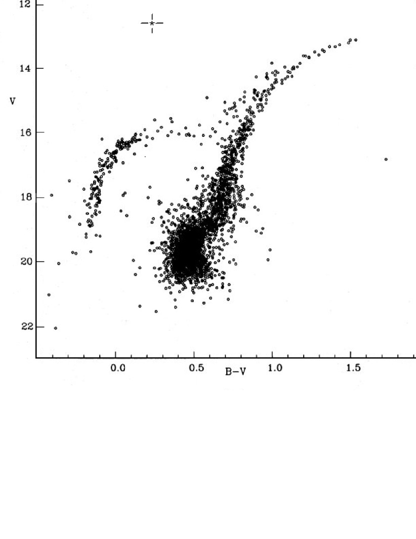
Figure 1: The colour-magnitude diagram of M79 with photometry from Ferraro et al. (1992). The PAGB star is marked by the cross.

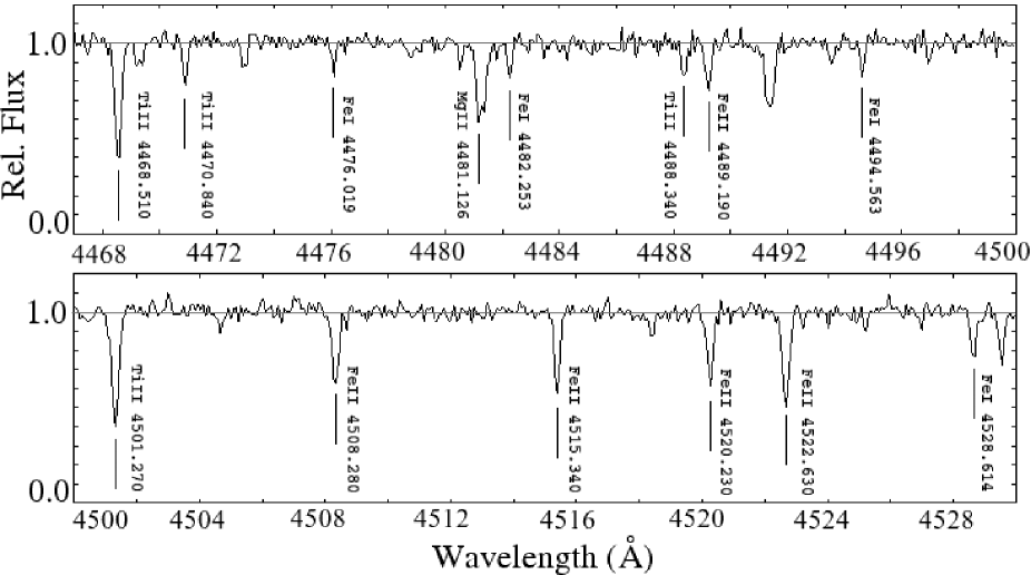
Figure 2: The spectrum for the PAGB star over the wavelength regions between 4467-4500 Å (upper panel) and 4500-4530 Å (lower panel). Selected lines are identified.

3 Abundance Analysis – The Model Atmospheres

The abundance analysis was undertaken with model atmospheres and the line analysis programme MOOG (Sneden 2002). The models drawn from the ATLAS9 grid (Kurucz 1993) are line-blanketed plane-parallel atmospheres in Local Thermodynamical Equilibrium (LTE) and hydrostatic equilibrium with flux (radiative plus convective) conservation. MOOG adopts LTE for the mode of line formation. A model is defined by the parameter set: effective temperature $T_{\rm eff}$, surface gravity $g$, chemical composition as represented by metallicity [Fe/H] and all models are computed for a microturbulence $\xi$ = 2 km s^-1. A model defined by the parameter set is fed to MOOG except that $\xi$ is determined from the spectrum and not set to the canonical 2 km s^-1 assumed for the model atmosphere. Several methods are available for obtaining estimates of the atmospheric parameters from photometry and spectroscopy. Most methods are sensitive to both $T_{\rm eff}$ and $\log g$ and, therefore, provide loci in the $T_{\rm eff}$ versus $\log g$ plane. We discuss several methods in an attempt to find consistent values for the effective temperature and gravity.

3.1 Photometry

Bond (2005, see also Siegel & Bond 2005) developed a photometric system with one of several aims being the detection of ‘stars of high luminosity in both young (yellow supergiants) and old (post-AGB stars) populations’. The system combines the Thuan-Gunn $u$ filter with the Johnson-Kron-Cousins $B$, $V$, and $I$ filters. Stellar parameters $T_{\rm eff}$ and gravity $g$ are obtainable from the colour-colour diagrams ($u-B$) versus ($B-V$) and $(u-B)-(B-V)$ versus $(V-I)$. Bond provides calibration diagrams for metallicities [Fe/H] = 0 and $-2$. Siegel (2008, private communication) reports the magnitudes of the M79 PAGB star to be $u$=13.803, $B$=12.480, $V$=12.203 and $I$=11.744. M79 is reddened by a negligible amount: $E(B-V)=0.01$ magnitudes (Heasley et al. 1986; Ferraro et al. 1992, 1999), a correction that is ignored here. This photometry and the [Fe/H] $=-2$ grid provides the following estimates ($u-B$) vs ($B-V$): $T_{\rm eff}=6400$K and $\log g=1.2$ cgs units.
$(u-B)-(B-V)$ vs $(V-I)$: $T_{\rm eff}=6300$K and $\log g=0.8$ cgs units.
The mean results are $T_{\rm eff}$=6350K and $\log g=1.0$ cgs units. Our abundance analysis indeed suggests that [Fe/H] $\simeq-2$. Analyses of the cluster’s red giants have, however, found [Fe/H] $\simeq-1.6$. Interpolation, necessarily crude given grids at only [Fe/H] = 0 and $-2$, suggests that for [Fe/H] $=-1.6$, the $T_{\rm eff}$ and $\log g$ are increased by 450 K and 0.8 dex, respectively. A calibration of the $(B-V)$ colour by Sekiguchi & Fukugita (2000) gives $T_{\rm eff}=6625$K (their equation 2) but the parameter space near [Fe/H]$=-2$ and $\log g=1.5$ is poorly represented by calibrating stars.

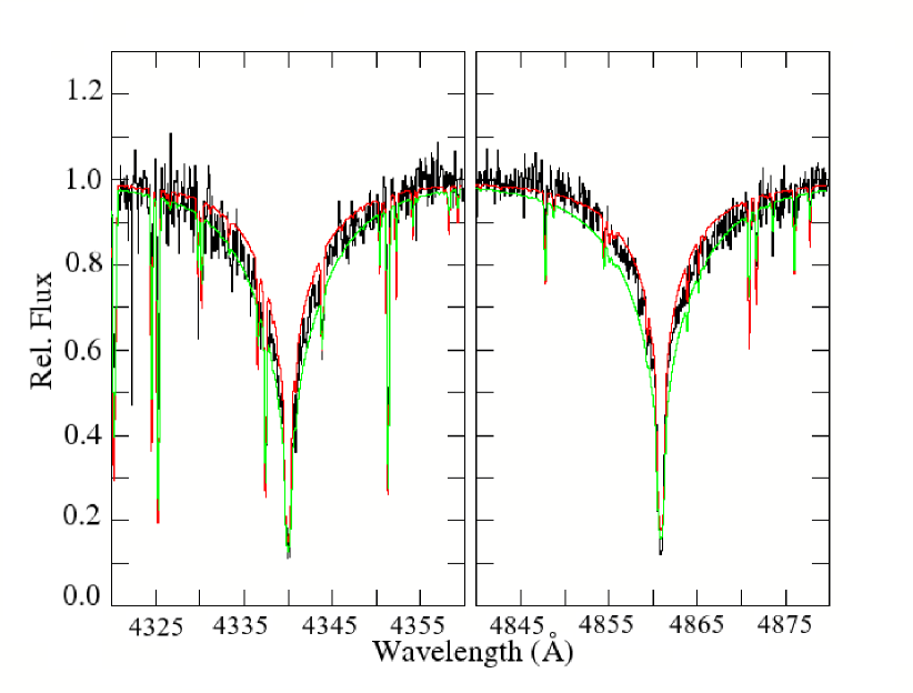
Figure 3: Observed and model line profiles for H$\beta$ and H$\gamma$. The theoretical profiles have been generated for a surface gravity $\log g=1.0$ dex and a metallicity [Fe/H]$=-2$. The red and green lines show the theoretical profiles for $T_{\rm eff}$= 6000 and 6500 K, respectively.

3.2 Balmer lines

The Balmer lines at temperatures around 6300 K are sensitive to $T_{\rm eff}$ with a weak dependence on gravity. The synthetic spectra for the Balmer lines H${\rm\beta}$ and H${\rm\gamma}$ have been computed with SYNTHE which is a suite of different programs , called one after the other by an input script with the purpose of producing a synthetic spectrum. These profiles were convolved with a gaussian profile in DIPSO to simulate the instrumental broadening. At $T_{\rm eff}<6000$ K, the theoretical H$\beta$ and H$\gamma$ profiles are narrower than the observed profiles for all plausible values of the surface gravity. At $T_{\rm eff}>6500$ K, the theoretical profiles are broader than the observed profiles. Acceptable fits are found for $T_{\rm eff}=6250$ K. A change of greater than $\pm 200$K in $T_{\rm eff}$ provides an unsatisfactory fit of theoretical to observed profiles. A gravity range of $\log g$ = 1.0 to 2.0 (and probably greater) does not impair the fit. In Figure 3, we show the observed profiles with theoretical line profiles for $T_{\rm eff}$=6000 K and 6500 K for $\log g=1.0$ and [Fe/H] $=-2$.

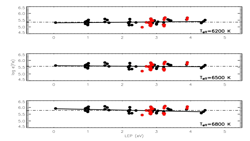
Figure 4: Iron abundances from individual Fe i (black filled circles) and Fe ii (red filled circles) lines versus a line’s lower excitation potential (LEP). Results are shown for three effective temperatures. The solid line in each plot is the least-squares fit to the abundances from the Fe i lines. The non-zero slope of this line for $T_{\rm eff}=6200$K and 6800K suggests that these values are too cool and too hot, respectively. The Fe ii lines in the mean are forced to provide the same Fe abundance as the Fe i lines by means of a different choice of surface gravity for each effective temperature (see text). The microturbulence velocity is 3.4 km s^-1.

3.3 Spectroscopy - Fe i and Fe ii lines

A selection of 42 Fe i lines was measured with lower excitation potentials (LEP) ranging from 0 to 4.4 eV and EWs of up to 170 mÅ but only three lines have EW greater than 100 mÅ. Measured Fe i and 25 Fe ii lines are listed in Table 1. The $gf$-values are taken from the recent critical compilation by Fuhr & Wiese (2006). In the limit that a line selection contains only weak lines, the $T_{\rm eff}$ is found by imposing the condition that the derived abundance be independent of the LEP. In the limit that all lines have the same LEP and a similar wavelength, the microturbulence $\xi$ is found by requiring that the derived abundance be independent of the EW. For our sample of Fe i lines, these two conditions must be imposed simultaneously. No species other than Fe i provides a sample of lines spanning an adequate range in LEP and EW to provide additional estimates of both $T_{\rm eff}$ and $\xi$. Solutions for $T_{\rm eff}$ and $\xi$ are not very sensitive to the adopted surface gravity. To illustrate the sensitivity to $T_{\rm eff}$, we show in Figure 4 the abundance-LEP relations for 6200 K, 6500 K, and 6800 K, i.e., $\pm 300$ K around the best value. It is to be noted that the slopes of the least-squares fitted relations are for 6200 K and 6800 K slight but possibly acceptable as different from zero.

Figure 5: The standard deviation of the Fe abundance from the suite of Fe i lines as a function of the microturbulence $\xi$ for a model with $T_{\rm eff}=6300$ K, $\log$ g = 0.8, and [Fe/H] $=-2$.

The microturbulence is determined separately from the Fe i and Ti ii lines. For a given model, we compute the dispersion in the Fe (or Ti) abundances over a range in the $\xi$. Figure 5 shows the dispersion $\sigma$ for Fe for $\xi$ from 0.5 to 7 km s^-1. A minimum value of $\sigma$ is reached at $\xi$ = 3.0 km s^-1 and a range of 2.2 km s^-1 to 5.0 km s^-1 covers the $\pm$50$\%$ range about the minimum value of $\sigma$. A value slightly less than $\xi=5$ km s^-1 is a firm upper limit because at higher values the predicted line widths exceed the observed widths, even if the macroturbulence is put at the unlikely value of 0 km s^-1. A similar exercise with the Ti ii lines gives $\xi=3.8$ km s^-1. We adopt a mean value of 3.4 km s^-1. These results are for a model with $T_{\rm eff}$ = 6300 K, $\log$ g = 0.8, and [Fe/H] =$-2$. Tests show that the derived $\xi$ is insensitive to these parameters over quite a wide range. Our abundances are primarily based on weak lines and are, thus, insensitive to the precise value of $\xi$. A third condition provides an estimate of the gravity. This is the familiar requirement that Fe i and Fe ii lines provide a single value of the Fe abundance. Obviously, this condition of ionization equilibrium provides a locus in the temperature-gravity plane running from low $T_{\rm eff}$ and low $g$ to high $T_{\rm eff}$ and high $g$ with the iron abundance increasing along this locus.

3.4 Ionization equilibria for Mg and Cr

Often, iron is the primary and occasionally the sole element used via ionization equilibrium to provide a $T_{\rm eff}-\log g$ locus which with an independent estimate of $T_{\rm eff}$ is used to obtain an estimate of $\log g$. The primary reason for iron’s supremacy is that it provides a plentiful collection of both neutral and ionized lines: here, 42 Fe i and 25 Fe ii lines. Our spectrum provides other elements with lines from the neutral and singly-ionized atoms, although much less well represented than iron. The elements in question are Mg and Cr for which the available lines are listed in Table 3. (The sources of the $gf$-values for these lines are identified in the subsequent discussion of elemental abundances.) Figure 6 shows that Mg, Fe and Cr loci in the $T_{\rm eff}-\log g$ plane.

3.5 Mass and Luminosity

An aspect of globular cluster membership is that one can estimate a star’s surface gravity from the known luminosity, effective temperature and a constraint on the estimated stellar mass. Combining the relations $L\propto R^{2}T_{\rm eff}^{4}$ and $g\propto M/R^{2}$, one obtains

$$\hskip 42.67912ptlogL/L_{\odot}=logM/M_{\odot}+4logT_{\rm eff}-logg-10.61$$ (1)

The absolute visual magnitude is $M_{V}=-3.37$. This with bolometric corrections from Fiorella Castelli (2008, private communication) provides estimates of $L/L_{\odot}$ as weak functions of $T_{\rm eff}$, $\log g$, and [Fe/H]: for example, $T_{\rm eff}$ = 6500K, $\log g$=1.5 and [Fe/H]= -2.0 give $L/L_{\odot}$ = 1740. This absolute luminosity is consistent with the range $L/L_{\odot}$ = 1070 to 1862 reported by Gonzalez & Lambert (1997) from five RV Tauri variables in other globular clusters and the theoretical characteristic that PAGB stars evolve at approximately constant luminosity. The mass of the PAGB star is less than 0.8$M_{\odot}$ and greater than the mass of white dwarfs in the cluster, say 0.5$M_{\odot}$ from mass estimates of the PAGB and white dwarfs in globular clusters (0.53$M_{\odot}$ is the typical PAGB remnant mass in NGC 5986 (Alves, Bond, & Onken 2001) and 0.50$\pm$0.02$M_{\odot}$ is the average mass of white dwarfs in nearby GCs and the halo field (Alves, Bond, & Livio 2000 and references therein). Adopting a mass of 0.6$M_{\odot}$, $T_{\rm eff}$=6500 K, and $L/L_{\odot}$ = 1740, we obtain the $\log g$=1.18. Extending this procedure to other $T_{\rm eff}$ gives a locus in the $T_{\rm eff},\log g$ plane but one which has a quite different slope to those from other indicators (Figure 6).

3.6 The Atmospheric Parameters

Figure 6 shows the loci discussed above. Convergence of the loci suggests adoption of the parameters ($T_{\rm eff}$ in K, $\log g$ in cgs) = (6300,0.8). The microturbulence $\xi=3.4$ km s^-1 is adopted from the Fe i and Ti ii lines analysis. The corresponding iron abundance is $\log\epsilon$(Fe) = 5.42 or [Fe/H] = $-2.03$ for the solar Fe abundance of $\log\epsilon$(Fe)=7.45 (Asplund et al. 2005). We refer to this model as the consensus choice. With these parameters, Fe ionization equilibrium is satisfied by design. Mg, and Cr ionization equilibria are quite well met: the abundance differences in the sense of neutral minus ionized lines is -0.1 dex for Mg and -0.2 dex for Cr. Also, there is a satisfactory fit to the Balmer line profiles, the excitation of the Fe i lines, and the $uBVI$ photometry. One is struck immediately by the fact that the consensus model yields a [Fe/H] that is lower by about 0.6 dex than the abundance previously derived for this cluster from its red giants (see Introduction). No modern abundance determination known to us has obtained a result near [Fe/H] $\simeq-2.0$. Adjustments for different assumptions about the solar Fe abundance will not reconcile previous and our results. As part of a preliminary exploration of ways to reconcile the composition of the PAGB star with that of the red giants, we report in Table 3 abundance analyses of the PAGB star for four model atmospheres falling along the ionization equilibrium track for iron: ($T_{\rm eff},\log g)$ = (6300,0.80), (6500,1.18), (6800,1.67), and (7000,1.98) where the final model returns essentially the Fe abundance reported for the cluster from its red giants. These abundances are obtained using the line selections described in the next section. In Table 3, the quantities $\log\epsilon$(X) and [X/Fe] reported by Carretta are given in columns two and three. In the next eight columns, we give our abundances and [X/Fe] computed from the solar abundances given by Asplund et al. (2005) which are given in the final column.

Figure 6: The $T_{\rm eff}$ versus $\log g$ plane showing the various loci discussed in the text. The loci include those derived from the fit to the Balmer line profiles H$\beta$ and H$\gamma$, the mass and luminosity estimates (L-M), the excitation of the Fe i lines, (FeI(ext)) and the imposition of ionization equilibrium for Mg (dashed line), Cr (solid line), and Fe (dashed line).

Table 1: Fe I and Fe II lines used in the analysis and corresponding abundances for the consensus model.

$$\begin{array}[]{@{}cc@{}r@{}c@{}rr||cc@{}r@{}c@{}rr@{}}\hline\cr\hline\cr$Species$&\lambda&$EW$&\log\epsilon(Fe)&$LEP$&\log(gf)&$Species$&\lambda&$EW$&\log\epsilon(Fe)&$LEP$&\log(gf)\\ &($\AA$)&(m$\AA$)&(dex)&($eV$)&&&($\AA$)&(m$\AA$)&($dex$)&($eV$)&\\ \hline\cr Fe$\,{\sc i}$&4383.540&167&5.1&1.49&0.20&Fe$\,{\sc i}$&5434.524&51&5.4&1.01&-2.12\\ Fe$\,{\sc i}$&4404.760&138&5.1&1.56&-0.14&Fe$\,{\sc i}$&5446.917&53&5.2&0.99&-1.91\\ Fe$\,{\sc i}$&4427.312&42&5.4&0.05&-3.04&Fe$\,{\sc i}$&5455.630&70&5.6&1.01&-2.09\\ Fe$\,{\sc i}$&4442.390&29&5.4&2.20&-1.26&Fe$\,{\sc i}$&5569.620&23&5.5&3.42&-0.49\\ Fe$\,{\sc i}$&4447.722&28&5.5&2.22&-1.34&Fe$\,{\sc i}$&5572.840&33&5.5&3.40&-0.28\\ Fe$\,{\sc i}$&4459.121&30&5.4&2.18&-1.28&Fe$\,{\sc i}$&5586.755&49&5.6&3.37&-0.14\\ Fe$\,{\sc i}$&4466.552&24&5.2&2.83&-0.60&Fe$\,{\sc i}$&5615.652&72&5.6&3.33&0.05\\ Fe$\,{\sc i}$&4476.019&21&5.4&2.85&-0.82&Fe$\,{\sc i}$&6494.980&24&5.4&2.40&-1.27\\ Fe$\,{\sc i}$&4482.253&31&5.7&2.22&-1.48&Fe$\,{\sc ii}$&4173.490&73&5.1&2.58&-2.61\\ Fe$\,{\sc i}$&4494.563&26&5.2&2.20&-1.14&Fe$\,{\sc ii}$&4303.200&96&5.4&2.70&-2.61\\ Fe$\,{\sc i}$&4528.614&61&5.4&2.18&-0.82&Fe$\,{\sc ii}$&4385.380&89&5.4&2.78&-2.58\\ Fe$\,{\sc i}$&4871.318&54&5.4&2.87&-0.36&Fe$\,{\sc ii}$&4416.817&92&5.4&2.78&-2.60\\ Fe$\,{\sc i}$&4872.138&33&5.4&2.88&-0.57&Fe$\,{\sc ii}$&4472.920&22&5.5&2.84&-3.53\\ Fe$\,{\sc i}$&4878.211&18&5.4&2.89&-0.89&Fe$\,{\sc ii}$&4489.190&58&5.4&2.83&-2.97\\ Fe$\,{\sc i}$&4957.593&134&5.7&2.81&0.23&Fe$\,{\sc ii}$&4508.280&117&5.5&2.86&-2.35\\ Fe$\,{\sc i}$&5001.860&28&5.6&3.88&-0.01&Fe$\,{\sc ii}$&4515.340&92&5.2&2.84&-2.36\\ Fe$\,{\sc i}$&5041.756&20&5.5&1.49&-2.20&Fe$\,{\sc ii}$&4520.230&87&5.4&2.81&-2.62\\ Fe$\,{\sc i}$&5049.819&16&5.2&2.28&-1.36&Fe$\,{\sc ii}$&4522.630&128&5.3&2.84&-1.99\\ Fe$\,{\sc i}$&5051.634&18&5.5&0.92&-2.80&Fe$\,{\sc ii}$&4555.890&97&5.2&2.83&-2.25\\ Fe$\,{\sc i}$&5139.463&48&5.5&2.94&-0.51&Fe$\,{\sc ii}$&4576.330&78&5.6&2.84&-2.92\\ Fe$\,{\sc i}$&5171.596&62&5.7&1.49&-1.79&Fe$\,{\sc ii}$&4582.840&70&5.7&2.84&-3.06\\ Fe$\,{\sc i}$&5191.455&32&5.4&3.04&-0.55&Fe$\,{\sc ii}$&4620.510&29&5.3&2.83&-3.19\\ Fe$\,{\sc i}$&5192.344&34&5.3&3.00&-0.42&Fe$\,{\sc ii}$&4629.340&101&5.2&2.81&-2.26\\ Fe$\,{\sc i}$&5194.942&29&5.6&1.56&-2.09&Fe$\,{\sc ii}$&4666.750&46&5.7&2.83&-3.37\\ Fe$\,{\sc i}$&5266.555&33&5.3&3.00&-0.39&Fe$\,{\sc ii}$&4731.440&50&5.6&2.89&-3.13\\ Fe$\,{\sc i}$&5270.356&68&5.4&1.61&-1.34&Fe$\,{\sc ii}$&5197.560&91&5.2&3.23&-2.05\\ Fe$\,{\sc i}$&5324.180&50&5.4&3.21&-0.10&Fe$\,{\sc ii}$&5234.620&112&5.6&3.22&-2.21\\ Fe$\,{\sc i}$&5367.500&26&5.6&4.42&0.44&Fe$\,{\sc ii}$&5264.810&34&5.7&3.23&-3.23\\ Fe$\,{\sc i}$&5369.962&27&5.5&4.37&0.54&Fe$\,{\sc ii}$&5276.000&109&5.2&3.20&-1.90\\ Fe$\,{\sc i}$&5383.369&30&5.3&4.31&0.65&Fe$\,{\sc ii}$&5325.560&40&5.1&3.22&-2.57\\ Fe$\,{\sc i}$&5397.128&78&5.3&0.92&-1.99&Fe$\,{\sc ii}$&5534.890&66&5.8&3.25&-2.86\\ Fe$\,{\sc i}$&5404.200&26&5.5&4.44&0.52&Fe$\,{\sc ii}$&6238.430&24&5.6&3.89&-2.75\\ Fe$\,{\sc i}$&5405.775&63&5.3&0.99&-1.84&Fe$\,{\sc ii}$&6456.390&72&5.7&3.90&-2.19\\ Fe$\,{\sc i}$&5429.696&86&5.5&0.96&-1.88&&&&&&\\ \hline\cr\hline\cr\end{array}$$

Table 2: Equivalent width measurements from the optical spectra. The corresponding abundances are presented for the consensus model.

$$\begin{array}[]{l@{}cr@{}rrr||l@{}cr@{}rcr@{}}\hline\cr\hline\cr$Species$&\lambda&$EW$&\log\epsilon(X)&$LEP$&\log(gf)&$Species$&\lambda&$EW$&\log\epsilon(X)&$LEP$&\log(gf)\\ &($\AA$)&(m$\AA$)&($dex$)&($eV$)&&&($\AA$)&(m$\AA$)&($dex$)&($eV$)&\\ \hline\cr C$\,{\sc i} $&9061.440&SS&\leq 5.7&7.48&-0.35&Ti$\,{\sc ii}$&4468.510&166&3.0&1.13&-0.62\\ C$\,{\sc i} $&9062.490&SS&\leq 5.7&7.48&-0.46&Ti$\,{\sc ii}$&4470.840&38&3.1&1.17&-2.28\\ C$\,{\sc i} $&9078.290&SS&\leq 5.7&7.48&-0.58&Ti$\,{\sc ii}$&4488.340&41&3.4&3.12&-0.82\\ O$\,{\sc i} $&8446.247&SS&8.0&9.52&-0.46&Ti$\,{\sc ii}$&4501.270&167&3.1&1.12&-0.75\\ O$\,{\sc i} $&8446.359&SS&8.0&9.52&0.24&Ti$\,{\sc ii}$&4529.480&61&3.5&1.57&-2.03\\ O$\,{\sc i} $&8446.758&SS&8.0&9.52&0.01&Ti$\,{\sc ii}$&4533.970&212&3.9&1.24&-0.77\\ O$\,{\sc i} $&9260.863&SS&\leq 8.0&10.74&-0.04&Ti$\,{\sc ii}$&4563.770&161&3.3&1.22&-0.96\\ O$\,{\sc i} $&9262.676&SS&\leq 8.0&10.74&0.09&Ti$\,{\sc ii}$&4571.960&185&3.6&1.57&-0.52\\ Na$\,{\sc i} $&8183.255&SS&\leq 4.0&2.10&0.24&Ti$\,{\sc ii}$&4708.650&35&3.0&1.24&-2.21\\ Na$\,{\sc i} $&8194.790&SS&\leq 4.0&2.10&-0.46&Ti$\,{\sc ii}$&4779.980&70&3.3&2.05&-1.37\\ Mg$\,{\sc i} $&4057.480&32&5.8&4.35&-0.90&Ti$\,{\sc ii}$&4798.530&30&3.0&1.08&-2.43\\ Mg$\,{\sc i} $&4167.230&26&5.6&4.35&-0.75&Ti$\,{\sc ii}$&4805.090&78&3.2&2.06&-1.12\\ Mg$\,{\sc i} $&4703.000&66&5.8&4.35&-0.44&Ti$\,{\sc ii}$&4874.010&24&3.1&3.10&-0.79\\ Mg$\,{\sc i} $&5183.620&201&5.7&2.72&-0.17&Ti$\,{\sc ii}$&5129.160&50&3.0&1.89&-1.40\\ Mg$\,{\sc i} $&5528.410&61&5.8&4.35&-0.50&Ti$\,{\sc ii}$&5154.070&66&3.4&1.57&-1.92\\ Mg$\,{\sc i} $&8806.760&153&6.2&4.35&-0.13&Ti$\,{\sc ii}$&5185.900&48&2.9&1.89&-1.35\\ Mg$\,{\sc ii}$&4481.126&SS&5.9&8.86&0.75&Ti$\,{\sc ii}$&5188.690&125&3.3&1.58&-1.22\\ Mg$\,{\sc ii}$&4481.150&SS&5.9&8.86&-0.55&Ti$\,{\sc ii}$&5211.544&28&3.2&2.59&-1.36\\ Mg$\,{\sc ii}$&4481.325&SS&5.9&8.86&0.59&Ti$\,{\sc ii}$&5336.780&57&3.1&1.58&-1.70\\ Si$\,{\sc ii}$&6347.091&SS&6.2&8.12&0.15&Ti$\,{\sc ii}$&5381.010&42&3.3&1.57&-2.08\\ Si$\,{\sc ii}$&6371.359&SS&6.2&8.12&-0.08&Ti$\,{\sc ii}$&5418.770&33&3.1&1.58&-1.99\\ Ca$\,{\sc i} $&4425.444&44&4.8&1.88&-0.36&Cr$\,{\sc i} $&4254.350&120&3.6&0.00&-0.11\\ Ca$\,{\sc i} $&4434.967&56&4.6&1.89&-0.01&Cr$\,{\sc i} $&4274.800&73&3.2&0.00&-0.23\\ Ca$\,{\sc i} $&4435.688&37&4.8&1.89&-0.52&Cr$\,{\sc i} $&4289.720&85&3.5&0.00&-0.36\\ Ca$\,{\sc i} $&4454.793&90&4.7&1.90&0.26&Cr$\,{\sc i} $&5204.510&38&3.6&0.94&-0.21\\ Ca$\,{\sc i} $&5588.764&31&4.5&2.53&0.21&Cr$\,{\sc i} $&5206.020&60&3.6&0.94&0.02\\ Ca$\,{\sc i} $&6102.722&25&4.8&1.88&-0.79&Cr$\,{\sc i} $&5208.420&58&3.4&0.94&0.16\\ Ca$\,{\sc i} $&6122.219&37&4.6&1.89&-0.32&Cr$\,{\sc ii}$&4242.380&40&3.7&3.87&-1.33\\ Ca$\,{\sc i} $&6162.172&57&4.6&1.90&-0.09&Cr$\,{\sc ii}$&4261.920&34&3.8&3.86&-1.53\\ Sc$\,{\sc ii}$&4246.840&182&1.3&0.32&0.24&Cr$\,{\sc ii}$&4555.016&20&3.5&4.07&-1.25\\ Sc$\,{\sc ii}$&4305.710&38&1.1&0.60&-1.21&Cr$\,{\sc ii}$&4558.660&67&3.6&4.07&-0.66\\ Sc$\,{\sc ii}$&4314.090&160&1.5&0.62&-0.10&Cr$\,{\sc ii}$&4592.090&30&3.6&4.07&-1.22\\ Sc$\,{\sc ii}$&4670.404&53&1.4&1.36&-0.58&Cr$\,{\sc ii}$&4616.640&40&3.9&4.07&-1.29\\ Sc$\,{\sc ii}$&5031.019&75&1.4&1.36&-0.40&Cr$\,{\sc ii}$&4618.820&53&3.9&4.07&-1.11\\ Sc$\,{\sc ii}$&5239.823&33&1.3&1.46&-0.77&Cr$\,{\sc ii}$&4634.100&32&3.7&4.07&-1.24\\ Sc$\,{\sc ii}$&5526.809&60&1.2&1.77&0.02&Cr$\,{\sc ii}$&4824.120&66&3.9&3.87&-1.23\\ Sc$\,{\sc ii}$&5657.870&40&1.3&1.51&-0.60&Cr$\,{\sc ii}$&4848.240&55&3.7&3.86&-1.13\\ Ti$\,{\sc ii}$&4367.657&63&3.1&2.59&-0.72&Cr$\,{\sc ii}$&4876.410&33&3.7&3.86&-1.47\\ Ti$\,{\sc ii}$&4386.850&34&3.3&2.60&-1.26&Cr$\,{\sc ii}$&5237.350&32&3.6&4.07&-1.16\\ Ti$\,{\sc ii}$&4394.020&61&3.0&1.22&-1.89&Cr$\,{\sc ii}$&5274.990&18&3.4&4.07&-1.29\\ Ti$\,{\sc ii}$&4395.830&74&3.5&1.24&-2.17&Mn$\,{\sc i} $&4030.753&SS&\leq 2.7&0.00&-0.48\\ Ti$\,{\sc ii}$&4407.680&32&3.2&1.22&-2.47&Ni$\,{\sc i} $&5476.910&SS&4.3&1.83&-0.89\\ Ti$\,{\sc ii}$&4411.100&47&3.3&3.10&-0.62&Sr$\,{\sc ii}$&4077.730&172&0.2&0.00&0.14\\ Ti$\,{\sc ii}$&4417.720&128&3.3&1.17&-1.43&Sr$\,{\sc ii}$&4215.540&159&0.2&0.00&-0.18\\ Ti$\,{\sc ii}$&4418.310&62&3.0&1.24&-1.82&Y$\,{\sc ii}$&4900.110&SS&\leq-0.3&1.03&-0.09\\ Ti$\,{\sc ii}$&4441.730&28&3.1&1.18&-2.41&Zr$\,{\sc ii}$&4208.980&SS&\leq 0.7&0.71&-0.51\\ Ti$\,{\sc ii}$&4443.820&162&3.0&1.08&-0.71&Ba$\,{\sc ii}$&5853.675&15&-0.1&0.60&-0.91\\ Ti$\,{\sc ii}$&4444.540&46&2.9&1.12&-2.03&Ba$\,{\sc ii}$&6141.718&75&0.0&0.70&-0.03\\ Ti$\,{\sc ii}$&4450.500&104&2.9&1.08&-1.45&Ba$\,{\sc ii}$&6496.897&57&0.1&0.60&-0.41\\ Ti$\,{\sc ii}$&4464.460&82&3.4&1.16&-2.08&Eu$\,{\sc ii}$&4205.050&30&-1.0&0.00&0.21\\ \hline\cr\hline\cr\end{array}$$

Table 3: Abundances of the observed species for M79 PAGB star are presented for four different model atmospheres. Also listed are abundances of the RGB stars in the same globular cluster analyzed by Carretta et al. (2008, private communication).

$$\begin{array}[]{@{}l||c@{}r@{}rrr||@{}c@{}}\hline\cr\hline\cr&&&(T_{\rm eff},\log\,g)&&&\\ \cline{2-6}\cr$Species$&$RGB$&$(6300,0.80)$&$(6500,1.18)$&$(6800,1.67)$&$(7000,1.98)$&\log\epsilon_{\odot}^{\star}\\ \cline{2-6}\cr&&&\log\epsilon(X),$[X/Fe]$&&&\\ \hline\cr\hline\cr C$\,{\sc i}$&...,...&\leq 5.7,\leq-0.7&\leq 5.7,\leq-0.8&\leq 5.9,\leq-0.8&\leq 6.0,\leq-0.9&8.39\\ O$\,{\sc i}$&7.29,+0.05&8.0,+1.4&8.0,+1.2&8.0,+1.0&7.9,+0.8&8.66\\ Na$\,{\sc i}$&5.05,+0.42&\leq 4.0,\leq-0.1&\leq 3.8,\leq-0.5&\leq 3.8,\leq-0.7&\leq 3.7,\leq-0.9&6.17\\ Mg$\,{\sc i}$&6.13,+0.28&5.8,+0.2&5.8,+0.2&6.0,+0.1&6.1,+0.1&7.53\\ Mg$\,{\sc ii}$&...,...&5.9,+0.4&6.0,+0.4&6.0,+0.1&6.0,+0.0&7.53\\ Si$\,{\sc ii}$^{\star}&6.24,+0.29&6.2,+0.7&6.2,+0.6&6.2,+0.4&6.3,+0.3&7.51\\ Ca$\,{\sc i}$&4.93,+0.28&4.7,+0.4&4.8,+0.4&4.9,+0.3&5.1,+0.3&6.31\\ Sc$\,{\sc ii}$&1.51,+0.04&1.1,+0.1&1.2,+0.1&1.5,+0.1&1.6,+0.1&3.05\\ Ti$\,{\sc ii}$&3.49,+0.07&3.2,+0.3&3.4,+0.4&3.6,+0.4&3.8,+0.4&4.90\\ Cr$\,{\sc i}$&3.96,-0.13&3.5,-0.1&3.7,-0.1&3.9,-0.1&4.1,-0.0&5.64\\ Cr$\,{\sc ii}$&4.14,-0.02&3.7,+0.1&3.8,+0.1&4.0,+0.1&4.1,-0.0&5.64\\ Mn$\,{\sc i}$&3.23,-0.53&\leq 2.7,\leq-0.7&\leq 2.9,\leq-0.6&\leq 3.1,\leq-0.6&\leq 3.3,\leq-0.5&5.40\\ Fe$\,{\sc i}$&5.96,+0.00&5.4,+0.0&5.6,+0.0&5.8,+0.0&5.9,+0.0&7.45\\ Fe$\,{\sc ii}$&5.94,+0.00&5.4,+0.0&5.6,+0.0&5.8,+0.0&5.9,+0.0&7.45\\ Ni$\,{\sc i} $&4.54,-0.16&4.3,+0.1&4.4,+0.1&4.7,+0.1&4.8,+0.2&6.23\\ Sr$\,{\sc ii}$&...,...&0.2,-0.7&0.4,-0.6&0.8,-0.5&1.0,-0.4&2.92\\ Y$\,{\sc ii}$&0.42,-0.27&\leq-0.3,\leq-0.5&\leq-0.1,\leq-0.4&\leq 0.2,\leq-0.3&\leq 0.4,\leq-0.3&2.21\\ Zr$\,{\sc ii}$&0.89,-0.16&\leq 0.7,\leq+0.1&\leq 0.9,\leq+0.2&\leq 1.1,\leq+0.2&\leq 1.4,\leq+0.4&2.59\\ Ba$\,{\sc ii}$&0.80,+0.13&0.0,-0.1&0.2,-0.1&0.5,+0.0&0.8,+0.2&2.17\\ Eu$\,{\sc ii}$&-0.62,+0.38&-1.0,+0.5&-0.8,+0.6&-0.5,+0.7&-0.2,+0.9&0.52\\ \hline\cr\hline\cr\end{array}$$

• ${}^{\mathrm{{{}^{\star}}}}$ The reported RGB abundance for silicon is from neutral silicon lines.

4 Abundance Analysis – Elements and Lines

For prospective elements, a systematic search was conducted for, as appropriate, lines of either the neutral and/or singly-ionized atoms with the likely abundance, lower excitation potential and $gf$-value as the guides. In this basic step, the venerable Revised Multiplet Table (Moore 1945) remains a valuable initial guide. When a reference to solar abundances is necessary in order to convert our abundance of element X to either of the quantities [X/H] or [X/Fe], we defer to Asplund et al. (2005). In general, many stellar lines are strong saturated lines in the solar spectrum and, therefore, a line-by-line analysis for the stellar-solar abundance differences is precluded. Carretta provided their adopted solar abundances which we use to convert their [X/Fe] to abundances $\log\epsilon$(X). In addition, they provided a list of lines which were the basis for the line selection made in the analysis of the red giants. A statistical comparison of the $gf$-values for common lines suggests that zero-point differences in abundances arising from different choices of $gf$-value between the RGB stars and the PAGB star are small. Our abundances are presented in Table 3 for the consensus model (6300, 0.80) and the three other models. An error analysis is summarized in Table 4 where we give the abundance differences resulting from models that are variously 300 K hotter, +0.2 dex of higher gravity, and experiencing a $\pm 0.5$ km s^-1 different microturbulence than the consensus model.

Comments on individual elements follow: C: Detection of C i lines was sought via the 3s³P^o-3p³P multiplet with lines between 9061Å and 9112Å. The multiplet is absent. The upper limit to the C abundance for the consensus model is $\log\epsilon$(C)$\leq 5.7$ from the 9061.44, 9062.49, and 9078.29Å lines with the $gf$-values from the NIST database. O: The O i triplet at 7774 Å is strong (Figure 7); an abundance $\log\epsilon$(O) $\simeq 8.0$ fits the triplet. The 8446 Å feature is present and provides an abundance $\log\epsilon$(O) $\simeq 8.0$ (Figure 7). The O i lines at 9260.8 Å and 9262.7 Å are absent and the upper limit $\log\epsilon$(O) $\leq 8.0$ is obtained. These consistent abundances correspond to the consensus model and to adoption of the NIST $gf$-values. Carretta (private communication) has noted that a correction for non-LTE effects lowers the 7774 Å abundance by about 0.6-0.8 dex. Corrections of a similar magnitude may apply to the other O i lines.

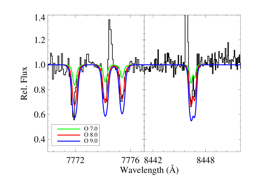
Figure 7: Observed and synthetic spectra around 7774 Å  and 8446 Å O i multiplets. The emission lines at 7774.5 and 8446.5 Å are night-sky emission OH lines.

Na: The Na D lines are prominent features in the spectrum (Figure 8). Three contributors are identifiable: strong stellar D lines, interstellar D lines with several blended components, and the night sky emission features which are not completely removed in the data reduction. The interstellar lines are similar as regards strength and velocity with the interstellar D lines reported by Gratton & Ortolani (1989) from spectra of two cluster red giants.

The Na abundance $\log\epsilon$(Na) $\simeq 5.5$ provides a fair fit to both D lines with the consensus model. However, as Figure 8 clearly shows, the stellar Na D lines are ill-suited for an abundance analysis as they fall on the ‘flat’ part of the curve of growth. The Na abundance is sensitive to small uncertainities in the measured EW and the adopted value of the microturbulence. The EW uncertainty of $\pm$13 mÅ translates to an abundance uncertainty of about $\pm$0.2 dex. A microturbulence uncertainty of $\pm 0.5$ km s^-1 corresponds to an abundance uncertainty of about $\pm$0.3 dex. Taking into account the $T_{\rm eff}$ sensitivity of (all) Na i lines, the likely uncertainty of a Na abundance derived from the D lines is in the range of $\pm$0.5 dex, even if LTE were valid.

In light of the inherent uncertainty in use of the Na D lines, we searched for weaker Na i lines. The leading candidates are the lines at 8183.3Å and 8194.8Å. Neither line is present in our spectrum. Spectrum synthesis gives the upper limit to the Na abundance as $\log\epsilon$(Na) $\leq 4.0$ for the consensus model, the value we adopt for the PAGB star. A Na abundance at this value provides Na D lines clearly much weaker than observed. We suppose that the predicted profiles for $\log\epsilon$(Na)=4.0 may be increased to match the observed D profiles by considering Na absorption from an extended (stationary) atmosphere, non-LTE effects, and/or an atmospheric structure different from that of the computed model atmosphere.

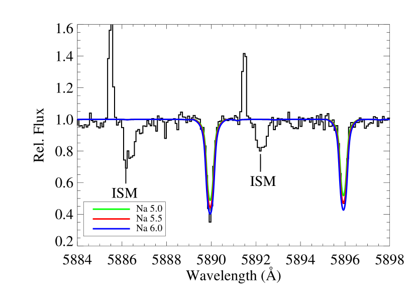
Figure 8: Observed and synthetic spectra around the 5895 Å Na i D lines. The interstellar Na D components are labelled ISM. Night-sky emission components are present.

Mg: Six Mg i lines are listed in Table 2 with their $gf$-values taken from the NIST database. Carretta et al. chose their $gf$-values from the same source. In calculating the mean Mg abundance from Mg i lines we drop the two strong lines (5183.6 Å and 8806 Å) as their derived abundances are sensitive to the adopted microturbulence and EW uncertainities.

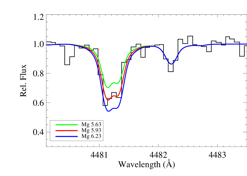
Figure 9: Observed and synthetic spectra around the 4481 Å Mg ii triplet lines.

For the Mg ii 4481Å feature, we take the $gf$-values also from the NIST database. Spectrum synthesis is used to provide the Mg abundance - see Figure 9. For the consensus model, the Mg abundances from the Mg i and Mg ii are 5.8 and 5.9, respectively.

Si: Silicon is represented solely by the Si ii lines at 6347 Å and 6371 Å. For the Si ii doublet, the $gf$-values are those recommended by Kelleher & Podobedova (2008, see also the NIST database). Spectrum syntheses for three Si abundances are shown with the observed spectrum in Figure 10. For the consensus model, the syntheses show that the abundance $\log\epsilon$(Si)=6.2 is a good fit to both lines with a poorer fit occurring for abundances differing by more than about $\pm$0.15 dex from this value.

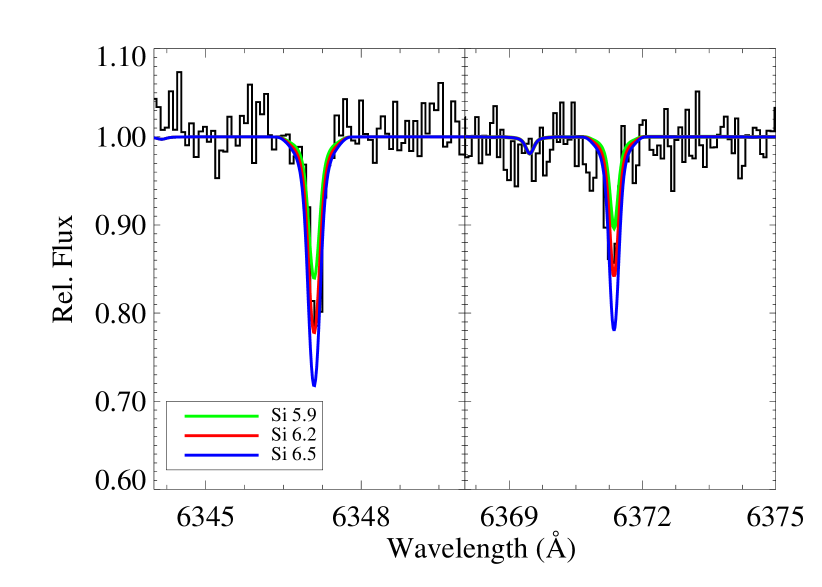
Figure 10: Observed and synthetic spectra around the 6347 and 6371 Å Si ii lines.

A search for Si i lines proved negative. The tightest limit on the Si abundance from Si i lines is obtained from a line at 7282.8 Å with the $gf$-value taken from Lambert & Warner (1968). This upper limit to the Si abundance is clearly in excess of that from the Si ii lines and the condition of ionization equilibrium, i.e., the constraint on the Si locus in Figure 6 is compatible with the loci for Mg, Cr, and Fe. Ca: The Ca abundance is based on the Ca i lines listed in Table 2 with their $gf$-values drawn from the NIST database. Carretta’s $gf$-values include NIST values but also Smith & Raggett’s (1981) measurements for some lines. The difference between our and Carretta’s $gf$-values varies from line to line but on average is probably small (say, $<0.05$ dex) and dependent on the particular line selection made by Carretta.

Sc: Our $gf$-values are taken with one exception from the NIST database. The exception is for the line at 4305Å which is in the NIST database but without an entry for the $gf$-value. For this line we adopt the value given by Gratton et al. (2003); Carretta adopts Gratton et al.’s recommendations for all Sc ii lines. With half weight given to the strongest lines (4246Å and 4314Å) and the 4305Å line with the non-NIST $gf$-value, the mean Sc abundance for the consensus and other models is given in Table 3. These mean abundances are approximately 0.1 dex greater than the value based on Gratton et al.’s $gf$-values. Ti: The search for Ti i lines was unsuccessful. The spectrum of Ti ii is well represented. For the ion, we take the $gf$-values from the NIST database. The exceptions are Ti ii lines at 4367, 4394, 4411, and 4418 Å. For 4394 Å line, we use $gf$-value from Roberts et al. (1973) and for the rest of four, $gf$-values from Ryabchikova et al. (1994) have been adopted. The abundances from NIST $gf$-values for these four differ from the mean of about $\pm 0.5$ dex. Carretta’s line list is also based on the NIST database. If a few outliers returning a high abundance are neglected, the Ti abundance from the Ti ii lines is independent of the EW of a line. The abundance for the consensus model is $\log\epsilon$(Ti) = 3.2. Cr: The Cr i lines in Table 2 have the well determined laboratory $gf$-values (Blackwell, Menon & Petford 1984; Tozzi, Brunner & Huber 1985) adopted for the NIST database and confirmed recently by Sobeck et al. (2007). Nilsson et al. (2006) from measurements of radiative lifetimes and branching ratios provide $gf$-values for many Cr ii lines, all with wavelengths short of 4850Å. The NIST database includes $gf$-values for all but three of our lines; Carretta adopts the NIST database. For six common lines, the mean abundance from Nilsson et al. is 0.01 dex smaller than from the NIST compilation. The dispersion from this subset of Cr ii lines is the same for both sets of $gf$-values. The Cr abundance from the Cr i lines is 3.5 and from the Cr ii lines is 3.7 dex from the consensus model. Mn: Lines of Mn are not detectable in our spectrum. The upper limit for the Mn abundance is best determined from the absence of the Mn i resonance lines near 4030Å with their $gf$-values known reliably from laboratory measurements for which we adopt the NIST database’s recommendations. For the consensus model, the upper limit is $\log\epsilon$(Mn) $\leq 2.7$. Carretta adopt NIST results for all Mn i lines in the spectra of the red giants. We assume that the RGB Mn abundance may be compared directly with the upper limit here determined. Fe: The $gf$-values for Fe i and Fe ii lines are from Fuhr & Wiese (2006). Carretta’s analysis of RGB stars uses $gf$-values from Gratton et al. (2003) that are essentially those of Fuhr & Wiese. Abundance analysis of our lines using the gf-value selection made by Gratton et al. gives an abundance only 0.06 dex higher from Fe i lines and 0.09 dex higher from Fe ii lines than our result. These differences indicate that the PAGB and RGB Fe abundances are essentially on the same scale. Ni: One Ni i line is listed in Table 2 with its $gf$-value from the NIST database. The Ni abundance for the consensus model is $\log\epsilon$(Ni) = 4.3. Carretta’s list of Ni i lines does not include this line but Carretta’s $gf$-values are essentially on the NIST scale. Sr: The Sr ii resonance lines at 4077Å and 4215Å are strong lines: Figure 11 shows these lines together with synthetic spectra. The $gf$-values are from Brage et al. (1998). These lines fall near the damping portion of the curve of growth and the derived abundance is, therefore, sensitive to the small uncertainties in the EWs, the microturbulence and to the damping (radiative) constant. The insensitivity of the predicted line profile to the Sr abundance is well illustrated by the synthetic spectra for Sr abundances of $-0.3$, $+0.2$, and $+0.7$.

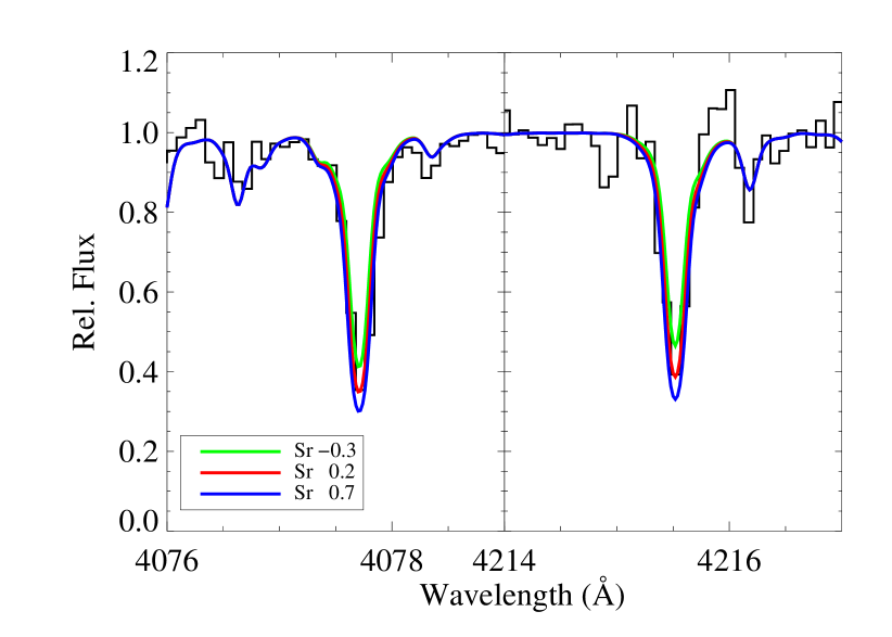
Figure 11: The observed spectrum around the Sr ii 4077.7 Å and 4215.5 Å  resonance lines.

Y: In our search for Y ii lines, Hannaford et al.’s (1982) list of clean solar Y ii lines with accurate $gf$-values was our starting point. Seven solar lines longward of 4300Å and with a solar EW greater than 35mÅ were considered. A representative line is included in Table 2: a series of synthetic spectra for this line at 4900.12Å  suggest an upper limit $\log\epsilon$(Y) $\leq-0.3$ for the consensus model. Zr: Our search for Zr ii lines drew on the papers by Biémont et al. (1981) and Ljung et al. (2006) who measured accurate laboratory $gf$-values and conducted an analysis of Zr ii lines to determine the solar Zr abundance. The strongest solar line identified with Zr ii is at 4208.98 Å. Synthetic spectra provide the upper limit $\log\epsilon$(Zr) $\leq 0.7$ for the consensus model.

Ba: The Ba ii resonance lines at 4554 Å and 4934 Å are present in great strength. The abundance analysis is based on the triplet of excited lines from the 5d²D levels at 5853 Å, 6141 Å, and 6496 Å with $gf$-values taken as the mean of the experimental values from Gallagher (1967) and Davidson et al. (1992). The lines have EWs such that consideration of hyperfine and isotopic splitting may be neglected. (The NIST $gf$-values for the resonance and these excited lines are erroneous. In compiling these values, it would appear that the absorption $f$-value given by Davidson et al. was treated as a $gf$-value, i.e., the NIST entries should be multiplied by the statistical weight $g$ of the lower level of the transition to obtain the $gf$-value.) Eu: The Eu ii resonance line at 4205.05Å is present.The weaker line at 4129.73 Å may be present. The $gf$-values are the accurate values provided by Lawler et al. (2001). The abundance is $\log\epsilon$(Eu) = $-1.0$ for the consensus model from the 4205 Å line with the 4129 Å line providing weak confirmation. The formal errors for the abundances arising from uncertainties of the atmospheric parameters – $T_{\rm eff},\log$ g, and $\xi$ – are summarized in Table 4 for changes with respect to the consensus model of $+300$K, $+0.2$ cgs units, and $\pm 0.5$ km s^-1 for the selected lines (i.e., the Na entries are based on the EW upper limits for the 8183 Å and 8194 Å lines). Given the estimated combined uncertainties and the dispersion in the line-to-line abundances for a given element, we elect to quote the abundances in Table 3 to one decimal place.

Table 4: Sensitivity of the derived abundances to the uncertainties in the model atmosphere parameters for the consensus model.

$$\begin{array}[]{@{}l||rrcc}\hline\cr\hline\cr&&\Delta log\,\epsilon&&\\ \cline{2-5}\cr$Species$&\Delta T_{\rm eff}&\Delta log\,g&\Delta\,\xi&\Delta\,\xi\\ \cline{2-5}\cr&$+300$&$+0.2$&$+0.5$&$-0.5$\\ &($K$)&($cgs$)&($km$\,s^{-1})&\\ \hline\cr C$\,{\sc i}$&-0.04&-0.05&\hskip 7.0pt0.00&0.00\\ O$\,{\sc i}$&-0.15&-0.09&-0.05&0.06\\ Na$\,{\sc i}$&+0.20&0.00&\hskip 7.0pt0.00&0.00\\ Mg$\,{\sc i}$&+0.17&-0.01&-0.02&0.02\\ Mg$\,{\sc ii}$&-0.10&+0.10&-0.05&0.15\\ Si$\,{\sc ii}$&-0.10&+0.05&-0.02&0.05\\ Ca$\,{\sc i}$&+0.22&-0.03&-0.03&0.03\\ Sc$\,{\sc ii}$&+0.11&+0.05&-0.05&0.05\\ Ti$\,{\sc ii}$&+0.12&+0.06&-0.07&0.10\\ Cr$\,{\sc i}$&+0.28&-0.01&-0.04&0.07\\ Cr$\,{\sc ii}$&+0.05&+0.06&-0.01&0.04\\ Mn$\,{\sc i}$&+0.35&-0.05&\hskip 7.0pt0.00&0.00\\ Fe$\,{\sc i}$&+0.25&-0.01&-0.03&0.04\\ Fe$\,{\sc ii}$&+0.08&+0.06&-0.05&0.08\\ Ni$\,{\sc i}$&+0.20&0.00&\hskip 7.0pt0.00&0.00\\ Sr$\,{\sc ii}$&+0.24&+0.05&-0.27&0.39\\ Y$\,{\sc ii}$&+0.15&+0.05&\hskip 7.0pt0.00&0.00\\ Zr$\,{\sc ii}$&+0.15&0.00&\hskip 7.0pt0.00&0.00\\ Ba$\,{\sc ii}$&+0.30&+0.03&-0.02&0.04\\ Eu$\,{\sc ii}$&+0.23&+0.04&-0.02&0.01\\ \hline\cr\hline\cr\end{array}$$

5 DISCUSSION

This exploration through quantitative spectroscopy of the newly discovered PAGB star in the globular cluster M79 has led to an unexpected and, therefore, fascinating result: the standard LTE analysis of the star has resulted in a metallicity different from that of the RGB stars analysed also by standard LTE techniques by Carretta. The consensus model of (6300,0.8) provides a [Fe/H] of $-2.0$ but the RGB analysis gives a [Fe/H] of $-1.5$. Here, we open a discussion of how one might account for this unexpected difference which exceeds a possible difference that might arise from uncertainties in the abundance analysis of these two different kinds of stars. Application of photometric and spectroscopic indicators of the atmospheric parameters for the PAGB star led to the consensus choice of $T_{\rm eff}=6300$ K and $\log g$=0.8. A model with these parameters (and a microturbulence $\xi=3.4$ km s^-1) fits not only the indicators but also the locus in the $T_{\rm eff}$ versus $\log g$ plane provided by the constraint on the star’s luminosity and mass. Table 3 summarizes the PAGB star’s composition for such a model atmosphere and contrasts it with the mean composition of the RGB stars. The PAGB star’s Fe abundance is $-0.5$ dex lower than that of the RGB stars. For the majority of the investigated elements, the difference in abundance $\log\epsilon$(X) in the sense (Ours $-$ Carretta) is within the range $-0.5\pm 0.3$ dex, i.e., the differences are equal to $-0.5$ dex to within measurement uncertainties. This result is readily seen from Table 3 by looking at the entries for [X/Fe] for elements measured in both the RGB and PAGB stars; The exceptions are O, Na, and Si. Strontium should be added to this trio because one anticipates that [Sr/Fe] $\simeq$ [Y/Fe] $\simeq$ [Zr/Fe] but [Sr/Fe] for the PAGB star is apparently 0.7 dex less than [Y/Fe] and [Zr/Fe] for the RGB stars. The exceptions of O and Na may be related. Carretta notes that the RGB stars show the O-Na correlation found in other globular clusters: high-Na paired with low-O. Here, the PAGB star has ([O/Fe],[Na/Fe]) = ($1.4,<-0.1$) but the mean for the 10 RGB stars is ($+0.05,+0.42$). A likely contributor to the explanation, as suggested by its lower Na abundance is that the PAGB star evolved from an RGB star largely uncontaminated with the products of the H-burning reactions that consume O and produce Na. The [O/Fe] of $+1.4$ is higher than expected for unevolved metal-poor stars. Estimated non-LTE effects on the O i 7770 Å triplet lines reduce the O abundance by about 0.6 – 0.8 dex. If similar corrections apply to the 8446 Å feature, the [O/Fe] would be cut from +1.0 to +0.2 – 0.4, an expected value for a metal-poor star as the value reported for the cluster’s RGB stars. (Carretta et al. used the [O i] lines that are unaffected by non-LTE effects.) The [X/Fe] for the PAGB star are generally consistent with expectation for metal-poor stars and, as noted above, generally equal to the measured values for the cluster’s RGB stars. The limit on [C/Fe] ($<-0.8$) indicates reduction of C by the first dredge-up and the absence of a C enrichment on the AGB. The [X/Fe] for the $\alpha$-elements (Mg, Ca, and Ti) at about $+0.3$ show the characteristic enhancement for metal-poor stars. Silicon is a notable exception – [Si/Fe] $=+0.7$ – for the PAGB star. The RGB stars have the expected value for [Si/Fe] of $+0.3$. This difference may be due to the use of the Si ii lines for the PAGB star and Si i lines for the RGB stars; non-LTE effects may have enhanced the strengths of the Si ii lines. Strontium was not measured in the RGB stars but our result [Sr/Fe] $=-0.7$ is, as noted above, strongly at odds with the RGB stars’ values of $-0.3$ for Y and $-0.2$ for Zr. This discrepancy is discussed below. Are these differences between the PAGB star and the RGB stars in [X/H] for many elements and [X/Fe] for a few elements intrinsic differences or reflections of systematic errors in the analyses? Certainly, the differences cannot be eliminated by an alternative choice of atmospheric parameters within the confluence of the various loci in Figure 6, i.e., models with $T_{\rm eff}$ within 300 K and $\log g$ within 0.3 dex of the consensus model (see Table 4). These questions we discuss next. Cluster RV Tauri variables analysed previously have not shown a clear [Fe/H] difference with the [Fe/H] of the RGB stars of the host cluster. Gonzalez & Lambert (1997) analysed variables in M2, M5, M10, and M28. With the exception of one variable in M5, the $T_{\rm eff}$ (spectroscopically derived from Fe i lines) were cooler than 5750 K. For three stars in clusters with [Fe/H] from $-1.2$ to $-1.6$, the RV Tauri star’s [Fe/H] was found to be within 0.1 dex of that from the RGB stars. The exception was a cluster (M10) with the RV Tauri star at $T_{\rm eff}=4750$ K giving [Fe/H]$=-2$ and with RGB stars showing [Fe/H]$=-1.5$ - an intriguing parallel with M79? The hottest variable in the sample (M5 V42, a star remarkable for the presence of Li) was reanalysed by Carney et al. (1998) using three spectra providing spectroscopic temperatures of 5200, 5500, and 6000 K. The [Fe/H] was $-1.2$ from each spectrum and equal to that from the cluster’s RGB stars. It is surely ironic that adoption of plane-parallel atmospheres for the analysis of these variable stars returns the same composition as their cluster’s RGB but the use of the model atmospheres for the (apparently) non-variable PAGB star in M79 gives rise to the abundance difference with the RGB stars.

5.1 Evolution and abundances

In the evolution of a RGB star to a PAGB star, there are several processes that may affect the surface compositions. At the tip of the RGB, the He-core flash and attendant mass loss may mix products of He burning to the surface. Evolution along the AGB following He-core burning may through the third dredge-up bring C and $s$-process products to the surface. Severe mass loss along and at the tip of the AGB may enhance changes in surface composition. Additionally, the surface composition of a PAGB star may be altered by processes unconnected to internal nucleosynthesis and dredge-up. PAGB stars have been found with abundance anomalies correlated with (i) the condensation temperature at which an element condenses out as dust or onto dust, and (ii) the ionization potential of the neutral atom, the so-called first ionization potential or FIP effect. Dust-gas separation, also referred to as winnowing, is possibly associated with a circumbinary dusty disk from which gas but not dust is accreted by the AGB and/or PAGB star (Van Winckel 2003). The signature of dust-gas winnowing is an underabundance correlated with the element’s predicted condensation temperature ($T_{\rm C}$). Observational examination of the dust-gas winnowing phenomena suggests that it is ineffective in intrinsically metal-poor stars, say [Fe/H] $<-1$ (Giridhar et al. 2005), and, therefore, is unlikely to have been effective in the M79 star, even were it a binary. Indeed, the RV Tauri stars in M2, M5, M10, and M28 (see Introduction) do not show evidence of dust-gas winnowing. Rao & Reddy (2005) show that field RV Tauri variables not portraying a clear signal of dust-gas winnowing may show abundance anomalies correlated with the ionization potential of the neutral atom (the FIP effect). Our search (see below) for an explanation of the composition difference between the PAGB and RGB stars in terms of nucleosynthesis and dredge-up, dust-gas winnowing, and the FIP effect proves negative.

5.1.1 Nucleosynthesis and dredge-up

The PAGB star’s C abundance is evidence that the PAGB star’s progenitor either did not experience C-enrichment from the third dredge-up or the enrichment was subsequently erased by (presumably) H-burning. The upper limit [C/Fe] $<-0.7$ is consistent with observations of other globular clusters that give [C/Fe] $<0$ with a decrease along the RGB, as anticipated from the first dredge-up. (Carretta does not report a C abundance for the RGB stars in M79.) Apparently, the He-core flash at the tip of the RGB and evolution from the horizontal branch to the AGB did not result in C enrichment from the addition of He-burning products to the atmosphere. Comparison of the heavy element abundances for the PAGB star with results for the RGB stars appears to provide a fascinating puzzle. For the RGB stars, Carretta reports [X/Fe] = $-0.27,-0.16,+0.13$ for Y, Zr, and Ba ($s$-process indicators) and $+0.38$ for Eu ($r$-process indicator), with [Fe/H] $=-1.6$. The star-to-star intrinsic variation in these [X/Fe] is less than the small observational uncertainties. These mean values are not at all unusual; field stars and stars in globular clusters of a comparable metallicity have these values (Gratton et al. 2004). For the PAGB star, our results are [X/Fe] = $<-0.5$, $<+0.1$ and $-0.1$ for Y, Zr, and Ba and $+0.5$ for Eu for the consensus model. The upper limits for Y and Zr are consistent with the values for the RGB stars. The [Ba/Fe] is less than for the RGB stars but possibly within the range of observational uncertainties considering that non-LTE effects have not been considered for either the PAGB star or the RGB stars. In short, there is no evidence that the PAGB star is a victim of $s$-processing on the AGB. Our [Eu/Fe]$\simeq+0.5$ matches the RGB stars’ Eu abundance. The outstanding puzzle is the Sr abundance of the PAGB star. The [Sr/Fe] $=-0.7$ is clearly at odds with [Y/Fe] $\simeq$ [Zr/Fe] $\simeq-0.2$ for the RGB stars. Moreover, among metal-poor stars – see the sample displayed by Lambert & Allende Prieto (2002) – the ratio [Sr/Ba] is positive but here [Sr/Ba] is highly negative ($-0.6$); the PAGB star would then be a remarkable outlier far from the representative sample shown by Lambert & Allende Prieto. It may be possible to conceive of a $s$-process scenario that reduces all three of these ratios yet keeps [Ba/Fe] close to the value for the RGB stars, but even highly contrived operating conditions for the $s$-process may not exist for producing the low [Sr/Fe] relative to [Y/Fe] and [Zr/Fe]. The key to the Sr problem may be that the Sr ii lines are strong and thus the Sr abundances are particularly uncertain with the microturbulence and non-LTE effects as major contributors to uncertainty. The consensus model adopts $\xi=3.4\pm 0.6$ km s^-1. If microturbulence is reduced to about $\xi=2.8$ km s^-1, the Sr abundance is raised to [Sr/H] $\simeq 0.7$ and [Sr/Fe] $\simeq-0.2$, a value consistent with the results for Y and Zr among the RGB stars. This value of $\xi$ is certainly not excluded by Figure 5. If one were confident that other effects (i.e., non-LTE) were not affecting the Sr ii lines in a serious way, one might use the Sr abundance to set $\xi$ for the abundance analysis. This alternative choice for $\xi$ has a minor effect on the other abundances except for the few elements represented exclusively by strong lines. The Sr ii line profiles may be fitted with this lower $\xi$ and a modest value for the macroturbulence. The key to resolving the Sr question will be observations of the 4d²D - 5p²P^o multiplet with lines at 10036.6 Å, 10327.3 Å, and 10914.9 Å.

5.1.2 Dust-gas winnowing and the FIP effect

A search for a correlation with the condensation temperature ($T_{\rm C}$) for an element returns a negative result. Some field RV Tauri variables show a striking correlation, e.g., HP Lyr (Giridhar et al. 2005). In HP Lyr, the Sc, and Ti underabundances at $T_{\rm C}\simeq 1600$ K are 2 dex greater than for Fe with $T_{\rm C}=1330$ K, Ca with $T_{\rm C}=1520$ K is 1 dex more underabundant, and Na at $T_{\rm C}=960$ K is 1 dex more abundant than Fe. For the consensus model, the [X/Fe] are here not correlated at all with $T_{\rm C}$. There is no indication that Sc and Ti in the PAGB star are underabundant relative to Fe and other elements of similar $T_{\rm C}$. Indeed, as noted above, the [X/Fe] of the PAGB star are not only generally equal to the values for the RGB star where dust-gas winnowing may be dismissed as a possible influence, but also essentially equal to the [X/Fe] expected for a metal-poor star. The Sr anomaly identified above is not attributable to dust-gas winnowing; the $T_{\rm C}$ of Sr is intermediate between that of Ca and Fe. Similarly there is no correlation of the abundances with the FIP.

5.2 Alternative choices of model atmosphere

If matching the [Fe/H] of the PAGB star to that of the RGBs is an overriding requirement in the selection of the model atmosphere parameters along with retention of the assumption of LTE in the model’s construction and the abundance analysis, one may pursue $T_{\rm eff},\log g$ combinations that lie along the line of Fe ionization equilibrium. A combination such as (7000, 1.98) is needed. Abundances for this and intermediate combinations are given in Table 3. This approach clearly provides Balmer line profiles that are far broader than the observed profiles (Figure 3), an Fe abundance from Fe i lines that decreases with increasing excitation potential (Figure 4). There is yet another problem raised by use of the (7000,1.98) model: this combination lies far off the locus set by the $L-M$ relation (Figure 6). To increase the $\log g$ from this relation requires an increase by 0.85 dex in the ratio $\log M/L$ (equation 1). Clearly, the allowable range on $M$ does not permit anything but a very small part of this increase. The major part has to be attributed to a decrease of the luminosity $L$. If one entertains the not implausible idea that the PAGB star may be affected by circumstellar dust, one immediately realises that extinction from a circumstellar dust shell aggravates the problem because the $L$ inferred from the magnitude $m_{V}$ is then increased not decreased. Luminosity $L$ may be decreased by a substantial reduction of the distance modulus but this negates the association of the star with M79. In short, matching the PAGB star’s Fe abundance to that of the RGB stars by choosing a much hotter classical model for the PAGB star that is consistent with the ionization equilibrium of Fe (and approximately Mg and Cr too) does not result in a satisfactory understanding of the PAGB star. This unsatisfactory state of affairs may in part arise because of the retention of the assumption of LTE. To first-order the principal non-LTE effect may be the over-ionization of Fe and similar metals. This over-ionization has a major effect on the strength of the lines of Fe i and similar metals. Since the Fe is predominantly present as Fe⁺, such non-LTE effects are weak for Fe ii lines. Also, effects of the overionization on the structure of the atmosphere are anticipated to be slight too because the additional contribution of electrons attributable to this non-LTE effect is very small. Thus, one might suppose that the Fe ii lines are a safe indicator of the PAGB star’s Fe abundance.

Discarding LTE in this way and raising the PAGB star’s Fe abundance from the Fe ii lines to the RGB stars’ value (where we assume non-LTE effects are minimal for the giants) requires a combination of a higher surface gravity and a higher effective temperature. The desired 0.6 dex increase in [Fe/H] is very difficult to achieve by sliding slightly the PAGB star along the $L-M$ relation; Table 4 shows that $T_{\rm eff}$ and $\log$g increases both raise the Fe abundance derived from the Fe ii lines. A very extreme slide to $T_{\rm eff}=7500$ K and $\log g=1.5$ increases the Fe abundance from Fe ii lines by the desired 0.5 dex. Thus, our simple assessment of likely non-LTE effects does not ease at all the reconciliation of the PAGB and RGB Fe abundances. One is seemingly forced to the conclusion that the model atmosphere may require substantial revision for the PAGB star. One concern is that the model atmospheres and the line analysis program assume a plane-parallel geometry but a spherical geometry may be more appropriate for the PAGB star. Heiter & Eriksson (2006) evaluated this concern for stars of solar metallicity and temperatures and gravities spanning the values of our PAGB star. Their conclusion is that abundance errors resulting from use of the plane-parallel geometry in model and line analysis rather than a consistent use of spherical geometry are minor provided that the analysis is restricted to weak (EW $<$ 100 mÅ) lines. Heiter & Eriksson express the expectation that this conclusion is likely valid too for low-metallicity stars and this was verified by Eriksson (2009, private communication) for this PAGB star. Apart from a few elements (e.g., Sr), our analysis is indeed based primarily on weak lines. Thus, the generally lower abundances for the PAGB star relative to the RGB stars are not attributable to use of the inappropriate geometry. An alternative representation of the model atmospheres seems necessary. Reproduction of the observed line strengths with the RGB star’s composition may be possible by invoking a departure from the structure of line-forming regions predicted by the ATLAS9 model. Two obvious qualitative possibilities are the presence of stellar granulation on small and/or large scales and a flatter temperature gradient over a uniform atmosphere. Such a change in gradient requires a different balancing of heating and cooling in the affected regions. Perhaps, convective transport of energy is inadequately modelled and/or ‘mechanical energy’ (e.g., acoustic waves) is supplied from the deep convective envelope. Of course, a revised atmospheric structure invalidates the determination of atmospheric parameters based on ATLAS9 models. Detailed exploration of semi-empirical atmospheres with might be undertaken to see how or if an atmospheric structure may be discovered that reconciles the wide variety of line strengths from the many elements with the composition of the RGB stars.

This suggestion about a failure of classical atmospheres to predict correctly the temperature gradient echoes a previous similar suggestion concerning the atmospheres of the R CrB stars, warm supergiants with a very H-deficient composition (Asplund et al. 2000). For those stars, the diagnostic indicating the failure was the strengths of the C i lines. The strengths of these lines should be quasi-independent of the atmospheric parameters because the continuous opacity is predicted to be from photoionization of carbon from levels only slightly greater in excitation than those providing the observed lines. These lines have very similar strengths across the R CrB sample (as expected) but the observed strengths are markedly weaker than predicted by classical (H-deficient) atmospheres. After a comprehensive review of a suite of possible explanations for this ‘carbon problem’, Asplund et al. proposed a flattening of the temperature gradient; the flattening investigated was assumed to apply to the entire atmosphere but it might possibly arise as a net effect of severe stellar granulation. The authors remarked that ‘spectra of (H-rich) F supergiants should be studied in attempts to trace similar effects’. This we have done for a star whose composition may be rather securely inferred from the RGB (and other) cluster members.

Although our study might appear to suggest that the ‘carbon problem’ affects H-rich as well as H-deficient supergiants, Galactic warm supergiants both in and out of the Cepheid instability strip may be innoculated against the ‘carbon problem’; the compositions determined spectroscopically are consistent with the various lines of evidence independent of spectroscopy that these stars must have an approximately solar metallicity. Thus, the parameter space over which the ‘carbon problem’ affects H-rich supergiants remains to be defined. Overall metallicity may be a key factor.

6 Concluding remarks

Our exploration of the PAGB star in M79 began with the expectation that either the star might show the canonical effects of the third dredge-up on the AGB (i.e., notably, a carbon and $s$-process enrichment) or the effects of dust-gas winnowing or the FIP effect. The exploration was derailed when it became apparent that an analysis using standard tools of the trade showed no evidence of expected abundance effects but rather an apparent 0.5 dex deficiency of iron and other elements. Qualitative considerations of how standard tools might be modified to effect an upward revision of the abundances by 0.5 dex led to the idea that the temperature profile of the PAGB’s atmosphere may be flatter than in a classical atmosphere.

Acquisition and analysis of a superior high-resolution spectrum may test our proposal concerning the atmospheric structure. It will not be difficult to improve upon the quality of our spectrum acquired with a ‘small’ (2.7 m) telescope: high S/N ratio and wavelength coverage are desirable. Detailed analysis of the spectral energy distribution, particularly across the Balmer jump may be valuable in assessing the temperature profile.

Our conclusion that standard model atmospheres are an inadequate representation of this post-AGB star would not have been drawn had the star not been a member of a globular cluster. For a field star, the conclusion would simply have been that [Fe/H] $=-2$ represented the star. The conclusion also suggests that abundance analyses of field PAGB stars may need reconsideration. Construction - empirically or theoretically - of more realistic model atmosphere will be very challenging but the task seems important if one is to unravel more completely the secrets of internal nucleosynthesis, dust-gas winnowing and the FIP effect that the post-AGB stars hold in the atmospheric compositions.

7 Acknowledgments

This research was begun when Howard Bond and Mike Siegel unselfishly alerted us to their discovery of the PAGB star in M79. We thank them both for the opportunity to analyse this interesting star. We are especially grateful to Eugenio Carretta for providing unpublished information on the composition of RGB stars in M79. We thank Fiorella Castelli for providing bolometric corrections for stars like the PAGB star in M79 and Bengt Gustafsson and Kjell Eriksson for offering comments on the use of spherical rather than plane-parallel atmospheres. This research has been supported in part by the grant F-634 from the Robert A. Welch Foundation of Houston, Texas.

References

- Alves, Bond, & Livio (2000) Alves, D. R., Bond, H. E., Livio, M., 2000, AJ, 120, 2044
- Alves & Bond (2001) Alves, D. R., Bond, H. E., Onken, C., 2001, AJ, 121, 318
- Asplund et al. (2000) Asplund, M., Gustafsson, B., Lambert, D.L., & Rao, N.K. 2000, A&A, 353, 287
- Asplund et al. (2005) Asplund, M., Grevesse, N., Sauval, A. J., 2005, in ASP Conf. Ser. 336, Cosmic Abundances as Records of Stellar Evolution and Nucleosynthesis, ed. T. G. Barnes III & F. N. Bash (San Francisco: ASP), vol. 336, 25
- Hannaford et al. (1981) Biémont, E., Grevesse, N., Hannaford, P., Lowe, R. M., 1981, ApJ, 248, 867
- Blackwell et al. (1984) Blackwell, D. E., Menon, S. L. R., Petford, A. D., 1984, MNRAS, 207, 533
- Bond (2005) Bond, H. E., 2005, AJ, 129, 2914
- Brage et al. (1998) Brage, T., Wahlgren, G. M., Leckrone, D. S., Proffitt, C. R., 1998, ApJ, 496, 1051
- Carney, Fry & Gonzalez (1998) Carney, B. W., Fry, A. M., Gonzalez, G., 1998, AJ, 116, 2984
- Davidson et al. (1992) Davidson, M. D., Snoek, L. C., Volten, H., Donszelmann, A., 1992, A&A, 255, 457
- Ferraro et al. (1992) Ferraro, F. R., Clementini, G., Pecci, F. F., Sortino, R., Buonanno, R., 1992, MNRAS, 256,391
- Ferraro et al. (1999) Ferraro, F. R., Messineo, M., Fusi Pecci, F., de Palo, M. A., Straniero, O., Chieffi, A., Limongi, M., 1999, AJ, 118, 1738
- Führ & Wiese (2006) Fuhr, J. R., Wiese, W. L., 2006, J. Phys. Chem. Ref. Data, 35, 1669
- Gallagher (1967) Gallagher, A., 1967, Phys. Rev., 157, 24
- Giridhar et al. (2005) Giridhar, S., Lambert, D. L., Reddy, B. E., Gonzalez, G., Yong, D., 2005, ApJ, 627, 432
- Gonzalez & Lambert (1997) Gonzalez, G., Lambert, D. L., 1997, AJ, 114, 341
- Gratton et al. (2003) Gratton, R. G., Carretta, E., Claudi, R., Lucatello, S., Barbieri, M., 2003, A&A, 404, 187
- Gratton & Ortolani (1989) Gratton, R. G., Ortolani, S., 1989, A&A, 211, 41
- Gratton et al. (2004) Gratton, R., Sneden, C., Carretta, E., 2004, ARA&A, 42, 385
- Hannoford et al. (1982) Hannaford, P., Lowe, R. M., Grevesse, N., Biémont, E., 1982, ApJ, 261, 736
- Harris (1996) Harris, W. E., 1996, AJ, 112, 1487
- Heasley et al. (1986) Heasley, J. N., Janes, K. A., Christian, C. A., 1986, AJ, 91, 1108
- Heiter & Eriksson (2006) Heiter, U., Eriksson, K., 2006, A&A, 452, 1039
- Kelleher & Podobedova (2008) Kelleher, D. E., Podobedova, L. I., 2008, J. Phys. Chem. Ref. Data, 37, 1285
- Kraft & Ivans (2003) Kraft, R. P., Ivans, I. I., 2003, PASP, 115, 143
- Kurucz (1993) Kurucz, R. L., 1993, ATLAS9 Stellar atmosphere Programs and 2 km grid CDRoM Vol 13 (Cambridge: Smithsonian Astrophysical Observatory)
- Kwok (1993) Kwok, S., 1993, ARA&A, 31, 63
- Lambert & Allende Prieto (2002) Lambert, D.L., Allende Prieto, C., 2002, MNRAS, 335, 325L
- Lambert & Warner (1968) Lambert, D. L., Warner, B., 1968, MNRAS, 138, 181
- Lawler et al. (2001) Lawler, J. E., Wickliffe, M. E., Den Hartog, E. A., 2001, ApJ, 563, 1075
- Ljung et al. (2006) Ljung, G., Nilsson, H., Asplund, M., Johansson, S., 2006, A&A, 456, 1181
- Mills & Webb (1994) Mills, D., Webb, J., 1994, Rutherford Appleton Laboratory, SUN 152.1
- Moehler (2001) Moehler, S., 2001, PASP, 113, 1162
- Moore (1945) Moore, C.E., 1945, ”A Multiplet Table of Astrophysical Interest”, Princeton Obs. Contr. No. 20 (reprinted 1959, Nat. Bur. Stand. Technical Note 36)
- Nilsson et al. (2006) Nilsson, H., Ljung, G., Lundberg, H., Nielsen, K. E., 2006, A&A, 445, 1165
- Rao & Reddy (2005) Rao, N. K., Reddy, B. E., 2005, MNRAS, 357, 235
- Roberts et al. (1973) Roberts, J. R., Andersen, T., Sørensen, G., 1973, ApJ, 181, 567
- Ryabchikova et al. (1994) Ryabchikova, T.A., Hill, G.M., Landstreet, J.D., Piskunov, N., Sigut, T.A.A., 1994, MNRAS, 267, 697
- Sekiguchi & Fukugita (2000) Sekiguchi, M., Fukugita, M., 2000, AJ, 120, 1072
- Siegel & Bond (2000) Siegel, M. S., Bond, H. E., 2005, AJ, 129, 2924
- Smith & Raggett (1981) Smith, G., Raggett, D. St. J., 1981, J. Phys. B, 14, 4015,
- Sneden (2002) Sneden, C., 2002, MOOG An LTE Stellar Line Analysis Program
- Sobeck et al. (2007) Sobeck, J. S., Lawler, J. E., Sneden, C., 2007, ApJ, 667, 1267
- Thompson et al. (2007) Thompson, H. M. A., Keenan, F. P., Dufton, P. L., Ryans, R. S. I., Smoker, J. V., Lambert, D. L., Zijlstra, A. A., 2007, MNRAS, 378, 1619
- Tozzi et al. (1985) Tozzi, G. P., Brunner, A. J., Huber, M. C. E., 1985, MNRAS, 217, 423
- Tull et al. (1995) Tull, R. G., MacQueen, P. J., Sneden, C. Lambert, D. L., 1995, PASP, 107, 251
- Van Winckel (2003) Van Winckel H., 2003, ARA&A, 41, 391
- Zinn & West (1972) Zinn, R., West, M. J., 1984, ApJS, 55, 45