Scaling of load in communications networks

Abstract

We show that the load at each node in a preferential attachment network scales as a power of the degree of the node. For a network whose degree distribution is $p(k)\sim k^{-\gamma},$ we show that the load is $l(k)\sim k^{\eta}$ with $\eta=\gamma-1,$ implying that the probability distribution for the load is $p(l)\sim 1/l^{2}$ independent of $\gamma.$ The results are obtained through scaling arguments supported by finite size scaling studies. They contradict earlier claims, but are in agreement with the exact solution for the special case of tree graphs. Results are also presented for real communications networks at the IP layer, using the latest available data. Our analysis of the data shows relatively poor power-law degree distributions as compared to the scaling of the load versus degree. This emphasizes the importance of the load in network analysis.

A variety of problems in fields ranging from the social sciences to biology to engineering deal with networks, for which a unified understanding has been sought bareview ; dorog ; newman . One of the models commonly used is the preferential attachment (PA) model due to Barabasi and Albert barabasi and its generalizations russian ; russian2 ; redner . This model generates scale-free networks, in which the probability for a node to have a degree $k$ scales as $p(k)\sim k^{-\gamma}.$ Depending on the parameters of the model, $\gamma$ can be varied continuously over the range $2<\gamma\leq 3.$ It has been argued that this model is appropriate to describe communications networks such as the Internet.

Among the various properties of PA networks that have been studied is the distribution of load (with uniform demand) at different nodes of the network. This is defined by assuming that one unit of traffic flows between each pair of nodes in the network along the shortest path connecting themfootbc . (If there are multiple shortest paths between a pair of nodes, the traffic between them is divided equally among all the shortest pathsfoot1 .) In this setting, the amount of traffic flowing through a node is its load. Based on numerical simulations goh , it was claimed that the probability distribution for the load scales as $p(l)\sim 1/l^{\delta}$ with $\delta=2.2.$ Subsequently, data for networks in various different fields were presented, and it was argued that goh2 there are two universality classes with $\delta=2$ and $\delta=2.2.$ These claims were disputed comment on the basis further numerical simulations, which seemed to indicate that $\delta$ varies continuously with $\gamma$ and is therefore not universal. For the special case of PA networks that are trees, it was argued szabo and then proved riordan that $\delta=2.$

In this paper, we show that the average load at nodes of degree $k$ scales as $l(k)\sim k^{\eta}$ with $\eta=\gamma-1$ for the PA model, regardless of $\gamma.$ (As $k$ is increased for fixed $N,$ finite size effects are seen.) If we assume that the distribution of load for fixed $k$ and $N$ does not have an anomalously large width, this implies that the exponent $\delta$ is universal, but is equal to 2, contradicting the earlier claims goh ; goh2 ; comment , and extending the exact result for PA trees. We also extend the analytical proof of Ref. riordan for tree graphs to show directly that $\eta=2,$ supporting the assumption that the distribution of $l$ for fixed $k$ is not anomalous. Our results are obtained by simple scaling arguments that are reinforced by finite size scaling studies. The deviations from this universal result that are observed goh ; comment are due to finite size scaling and subleading corrections to the asymptotic scaling form.

We also show results for load analyses on networks drawn from a recent database rocketfuel of connectivity of communications networks at the IP layer. The data are collected with new measurement techniques, and find many more routers and links than earlier studies f3 . The results demonstrate that the scaling of the load $l(k)\sim k^{\eta}$ is much clearer than that of the —more commonly studied— degree distribution.

In the generalized PA model, a network grows one node at a time. Each node is born with $m$ undirected edges which are attached to preexisting nodes. The probability of attachment to a preexisting node of degree $k$ is proportional to $k+k_{0}.$ Thus $k_{0}$ and $m$ are the parameters of the model, with $k_{0}<-m.$ For an infinite network, it can be shown that the probability of a randomly chosen node having a degree $k$ is to

$$p_{k}\propto k^{-\gamma}\qquad\gamma=3+k_{0}/m$$ (1)

for large $k.$ For such a network, we assume —as verified later through numerical simulations— that the average load $l_{N}(k)$ at all the nodes of degree $k$ in a network of $N$ nodes has the scaling form

$$l_{N}(k)=Nk^{\eta}\hat{l}(k/N^{\mu})$$ (2)

where $\hat{l}(x)\rightarrow 1$ as $x\rightarrow 0$ and $\hat{l}(x)\rightarrow 0$ as $x\rightarrow\infty.$ The prefactor of $N$ is reasonable, since most of the load at nodes near the periphery of the network, for which $k\sim O(1)$, is due to traffic that starts or ends there, and is therefore $O(N).$ The exponent $\eta$ can be found by noting that $\sum_{k}[Np_{k}]l_{N}(k)$ is the total traffic flowing in the network. Since $N^{2}$ units of traffic are generated in the graph, and the average geodesic length is $\sim\ln N,$ the sum should scale as $\sim N^{2}\ln N$ for large $N.$ From Eqs.(1) and (2), this implies that

$$\eta=\gamma-1.$$ (3)

To find the exponent $\mu,$ we note that for a network of $N$ nodes, the maximum degree $k_{max}$ that is achieved can be estimated by requiring $(1-\sum_{k_{max}}^{\infty}p_{k})^{N}$ to be $\sim O(1).$ From Eq.(1), for large $k_{max}$ this is equivalent to $\exp[-AN/k_{max}^{\gamma-1}]\sim O(1)$ with some constant $A,$ from which $k_{max}\sim N^{1/(\gamma-1)}.$ If we assume that all characteristic $k$’s scale with $N$ in the same way, we obtain

$$\mu=1/(\gamma-1).$$ (4)

For $k<<N^{\mu},$ Eq.(2) implies that $l_{N}(k)\sim Nk^{\eta}.$ When combined with Eq.(1), we have $p(l)dl\sim dl/l^{\delta}$ with

$$\delta=\frac{\gamma-1}{\eta}+1=2$$ (5)

where we have used Eq.(3).

Although these results are plausible, they are based on assumptions, most notably the scaling hypothesis of Eq.(2) itself. To check these assumptions, we turn to finite size scaling numerical simulations. Networks with $N$ ranging from 500 to 8000 or 16000 were generated for different values of $m$ and $k_{0}.$ We considered the cases $k_{0}=0$ with $m=1,2,4,6$ and $m=6$ with $k_{0}=1,2,3,4,5.$ For each choice of $k_{0},m$ and $N,$ 10000 graphs were generated, with traffic flowing as described above. $l_{N}(k)$ was calculated by averaging over all the nodes of degree $k$ in the 100 graphs. For the plots, it is more convenient to use the form $l_{N}(k)=N^{2}\tilde{l}(k/N^{\mu})$ instead of Eq.(2), which one obtains if one uses Eqs.(4) and (3).

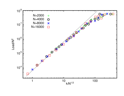
Figure 1: Average traffic at nodes of degree $k$ as a function of $k$ for the PA model with $m=1,k_{0}=0.$ (Here and in the subsequent figures, $N/8000$ is used to scale both axes instead of $N.$) A scaling collapse with the exponents from Eqs.(3) and (4) works reasonably well. However, a straight line with the predicted slope of 2.0 is shown and only fits the curve — if at all — for small $k.$ Similar deviations are seen for $m=2,4,6$ with $k_{0}=0.$

Figure 1 shows the results for $m=1$ and $k_{0}=0,$ for which $\mu=1/2$ from Eq.(4). The scaling collapse is reasonable, but the best fit straight line is in fact $l(k)\sim k^{1}.8,$ consistent with earlier results szabo . In view of the analytical results for PA tree graphs, this discrepancy must be attributed to finite size scaling effects which flatten the curve for large $k$ and presumably reduce the apparent value of $\eta.$ The same discrepancy is seen for $k_{0}=0$ with $m=2,4,6$; it is reasonable to attribute it to the same cause.

Figure 2: Scaling plot of the average traffic at nodes of degree $k$ as a function of $k$ for the PA model with $m=6,k_{0}=3.$ The scaling collapse is very good, as is the fit to $\sim k^{3/2}$ in the scaling regime.

Figure 2 shows a similar scaling plot for $m=6$ and $k_{0}=3,$ for which $\mu=2/3.$ The scaling collapse and the fit to $l(k)\sim k^{1}.5$ are both very good in this case. Figure 3 is a similar plot for $m=6$ and $k_{0}=5.$ The scaling collapse is again very good, but finite size corrections for large $k$ now increase the slope of the curve. Thus the fit to the predicted form of $\sim k^{7/6}$ only works when $k<<N^{6/7}$ but $k>>O(1).$ ( Unless the scaling hypothesis breaks down, Eq.(3) follows from the $\ln N$ factor in the total load. Therefore, we do not try a scaling plot with adjustable exponents..) We have also made similar plots for $m=6$ and $k_{0}=1,2$ and 4. For $k_{0}<3,$ finite size corrections reduce the apparent $\eta$ for large $k,$ while for $k_{0}>3,$ they increase the apparent $\eta$ for large $k.$ This is consistent with Ref. comment .

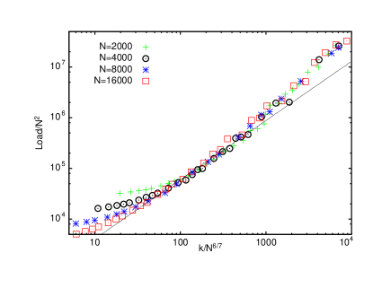
Figure 3: A plot similar to Figure 2 but with $k_{0}=5.$ For $k\sim O(1),$ the individual curves pull away from the scaling form. For $k\sim O(N^{6/7}),$ finite size effects cause the curves to bend upwards. Between these two regimes, the slope is consistent with $\sim k^{7/6}$ as predicted.

For the tree graphs generated by the PA model with $m=1,k_{0}=0,$ the result $l(k)\sim k^{2}$ follows from $p(k)\sim 1/k^{3}$ and $p(l)\sim 1/l^{2}$ if we assume that $l(k)$ scales as a power of $k$ and that the distribution of $l$ for fixed $k$ is not anomalously broad. Although these are reasonable assumptions, it is not difficult to prove $l(k)\sim k^{2}$ directly. The probability that the node created at time $\tau$ will be attached to a preexisting node of degree $k$ is equal to $k/(2\tau-2).$ Therefore the probability that a node created at time $\tau$ will have exactly $k$ nodes subsequently attached to it is

$$p_{k+1,N}(\tau)=\sum_{\tau<\tau_{1}<\ldots\tau_{k}}^{N}P(\tau+1,\tau_{1}-1,1)\frac{1}{2(\tau_{1}-1)}P(\tau_{1}+1,\tau_{2}-1,2)\frac{2}{2(\tau_{2}-1)}\ldots P(\tau_{k-1}+1,\tau_{k}-1,k)\frac{k}{2\tau_{k}-2}P(\tau_{k}+1,N,k+1)$$ (6)

where

$$P(\tau,\tau^{\prime},m)=\Bigg{(}1-\frac{m}{2\tau-2}\Bigg{)}\Bigg{(}1-\frac{m}{2\tau}\Bigg{)}\ldots\Bigg{(}1-\frac{m}{2\tau^{\prime}-2}\Bigg{)}.$$ (7)

Replacing $P(\tau,\tau^{\prime},m)$ as the exponential of an integral instead of a sum in the approximation $\tau>>1,$ we have $P(\tau,\tau^{\prime},m)=(\tau/\tau^{\prime})^{m/2}.$ With this, Eq.(6) simplifies to

$$p_{k+1,N}(\tau)\approx\sum_{\tau_{1}=\tau}^{N}\ldots\sum_{\tau_{k}=\tau}^{N}\sqrt{\frac{\tau}{N}}\frac{1}{2\sqrt{\tau_{1}N}}\ldots\frac{1}{2\sqrt{\tau_{k}N}}$$ (8)

where we have used the symmetry of the $\tau_{i}$’s to eliminate the restriction $\tau_{1}<\tau_{2}\ldots<\tau_{k}.$ If the sums are replaced with integrals, $p_{k+1,N}(\tau)=\sqrt{\tau/N}[1-\sqrt{\tau/N}]^{k}$kr and $p_{k}=(1/N)\sum_{\tau}p_{k,N}(\tau)\sim 1/[k(k+1)(k+2)]$ for large $N.$

If $n_{1},n_{2},\ldots n_{k}$ are the sizes of the $k$ subtrees descending from a node of degree $k+1,$ one can show riordan that for large $N$ the load at the node is proportional to $N\sum n_{i}.$ If $n_{i}(t)$ is the size of the $i$’th subtree at time $t\geq\tau_{i},$ with $n_{i}(N)=n_{i},$ the probability that $n_{i}(t+1)=n_{i}(t)+1$ is $(2n_{i}-1)/(2t),$ with the initial condition $n_{i}(t)=1.$ at time $t.$ Averaging over randomness for fixed $\tau_{i},$ the solution is $\langle n_{i}(t)\rangle=(t/\tau_{i}+1)/2.$ With the symmetrization of the previous paragraph,

$$l_{N}(k+1;\tau)\propto N\langle\sum n_{i}\rangle=Nk\langle n_{i}\rangle=\frac{kN}{1-x}\int_{x}^{1}\frac{1+x_{i}^{2}}{x_{i}^{2}}dx_{i}$$ (9)

where $\tau_{i}=Nx_{i}^{2},\tau=Nx^{2}$ and we have replaced sums with integrals. This yields

$$l_{N}(k+1)\propto Nk^{3}\int_{0}^{1}x(1-x)^{k}[2k(1+x)+x]dx\propto Nk^{2}$$ (10)

where we have only kept the terms that are relevant for $N>>k>>1.$ The terms dropped with the $k>>1$ approximation are corrections to asymptotic scaling and cause the imperfect collapse in Figure 1 .

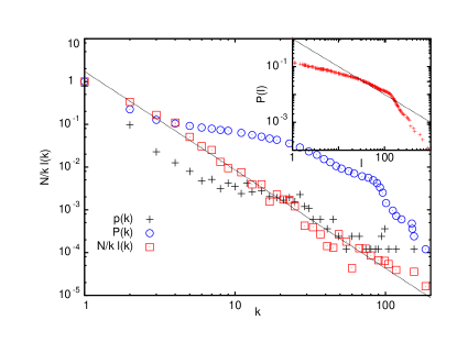
Figure 4: Log log plot of $N/(kl(k))$ as a function of $k$ for the Sprintlink network rocketfuel . The dashed line is visually adjusted for best fit, and has a slope of $-2.3$ corresponding to $l(k)\sim k^{\eta}$ with $\eta=1.3.$ The plot also shows the degree distribution $p(k)$ and the cumulative distribution $P(k)=\sum_{k}^{\infty}p(k_{1}).$ The inset shows the cumulative load distribution $P(l)=\int_{l}^{\infty}p(l_{1})dl_{1}$ and a straight line with slope -1.

We now compare with network data from the Rocketfuel database rocketfuel , which is the most recent, comprehensive and publicly available collection of measurements of the connectivity between nodes of communications networks at the IP layer. There are ten networks with 121 to 10214 routing nodes (from here on referred to as ”routers”) in the database. Since the data is insufficient to test scaling functions (in our simulations we worked with 100 networks for each $N,$ with $500<N<\sim 10000$), we only consider how the traffic at nodes scales with their degree without regard to any finite size cutoff. Figure 4 shows the results for one of the larger networks in the database, the Sprintlink network with 8355 routers. The load as a function of degree fits quite well to a power law with a slope of 1.3. The degree distribution itself is much more irregular, and it is difficult to say whether it is of the form $\sim k^{-\gamma}$ with $\gamma=\eta+1.$ The cumulative degree distribution is also shown in the figure; it is much smoother, but does not show clear power law behavior. The inset shows the cumulative load distribution and a straight line with the predicted slope of -1, which is equally unconvincing. Figure 5 is a similar figure with all ten networks in the database merged. The plots are straighter, and one could perhaps argue for a narrow power law regime in the cumulative degree distribution as is done in Ref. rocketfuel or a regime with slope $-1$ in the inset. However, the load versus degree has a much closer linear behavior in the log-log plot, and is therefore a more natural demonstration of power-law scaling in communications networks than the more commonly studied degree distribution.

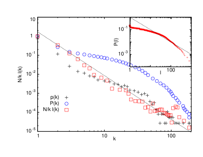
Figure 5: Plot similar to Figure 4 but with results from all ten networks in the database combined.

In conclusion, we have shown that for a preferential attachment model with degree distribution $p(k)\sim k^{-\gamma},$ the average traffic as a function of node degree scales as $l(k)\sim k^{\gamma-1}.$ This is equivalent to the statement that the probability distribution for the load scales as $p(l)\sim 1/l^{2}$ regardless of $\gamma.$ Although the numerical simulations and analytical calculations are for a specific model, the result follows from the scaling assumption and the small-world phenomenon and is therefore more robust. The scaling $l(k)\sim k^{\eta}$ is also seen clearly in networks at the IP layer, and is in fact much better than the degree distribution which has attracted much more interest.

This work was supported by AFOSR grant FA9550-08-1-0064.

References

- (1) R. Albert and A.-L. Barabasi, Rev. Mod. Phys. 74, 47 (2002).
- (2) S.N. Dorogovtsev and J.F.F. Mendes, Adv. Phys. 51, 1079 (2002).
- (3) M.E.J. Newman, SIAM Review 45, 167 (2003).
- (4) A.-L. Barabasi and R. Albert, Science 286, 509 (1999).
- (5) S.N. Dorogovtsev, J.F.F. Mendes and A.N. Samukhin, Phys. Rev. Lett. 85, 4633 (2000).
- (6) S.N. Dorogovtsev and J.F.F. Mendes, Phys. Rev. E 63, 056125 (2001).
- (7) P.L. Krapivsky, S. Redner and F. Leyvraz, Phys. Rev. Lett. 85, 4629 (2000).
- (8) This notion of load is sometimes referred to as “betweenness centrality”.
- (9) We do not distinguish between geodesics that are partly overlapping and those that are completely distinct. Thus if there are three geodesics between a pair of nodes, with the first two overlapping for most of their lengths and the last one completely separate, the traffic along each would be resulting in greater traffic over most of the overlapping geodesics.
- (10) K-I. Goh, B. Kahng and D. Kim, Phys. Rev. Lett. 87, 278701 (2001).
- (11) K-I. Goh, E. Oh, H. Jeong, B. Kahng and D. Kim, Proc. Natl. Acad. Sci, 99, 12583 (2002).
- (12) M. Barthelemy, Phys. Rev. Lett. 91, 189803 (2003).
- (13) G. Szabo, M. Alava and J. Kertesz, Phys. Rev. E 66, 026101 (2002).
- (14) B. Bollobas and O. Riordan, Phys. Rev. E 69, 036114 (2004).
- (15) N. Spring, R. Mahajan, D. Wetherall, Proc. ACM/SIGCOMM ’02, 133 (2002). Data archive at http://www.cs.washington.edu/research/networking/rocketfuel/.
- (16) M. Faloutsos, P. Faloutsos and C. Faloutsos, Proc. ACM/SIGCOMM ’99, 251 (1999). For a discussion of the difficulties in interpreting this data, see for instance Q. Chen, H. Chang, R. Govindan, S. Jamin, S.J. Shenker and W. Willinger, Proc. INFOCOM 2002, 608 (2002).
- (17) P.L. Krapivsky and S. Redner, Phys. Rev. E 63, 066123 (2001).