ACCELERATING COSMOLOGY IN RASTALL’S THEORY

Abstract

In an attempt to look for a viable mechanism leading to a present-day accelerated expansion, we investigate the possibility that the observed cosmic speed up may be recovered in the framework of the Rastall’s theory, relying on the non-conservativity of the stress-energy tensor, i.e. $T^{\mu}_{\nu;\mu}\neq 0$. We derive the modified Friedmann equations and show that they correspond to Cardassian-like equations. We also show that, under suitable assumptions on the equation of state of the matter term sourcing the gravitational field, it is indeed possible to get an accelerated expansion, in agreement with the Hubble diagram of both Type Ia Supernovae (SNeIa) and Gamma Ray Bursts (GRBs). Unfortunately, to achieve such a result one has to postulate a matter density parameter much larger than the typical $\Omega_{M}\simeq 0.3$ value inferred from cluster gas mass fraction data.

I Introduction

The observed cosmic speed up Riess98 ; Perlmutter99 ; Bennet et al. (2003) questions the validity of General Relativity (GR) on large scales. In fact, if on one hand the model of gravitational interaction as described by Einstein’s theory is in agreement with many observational tests on relatively small scales, as Solar System and binary pulsars observations show Will06 , it is well known that in order to make GR agree with the observed acceleration of the Universe the existence of dark energy, a cosmic fluid having exotic properties, has been postulated. Actually, many candidates for explaining the nature of dark energy have been proposed (see e.g. peebles03 , dark and references therein), some of them relying on the modification of the geometrical structure of the theory, some others on the introduction of physically (up to day) unknown fluids into the equations governing the behaviour of our universe. Moreover, it is interesting to point out that the problem of explaining the acceleration of the Universe has been addressed also in the framework of GR (see kolb and references therein).

In this context, we want to consider here a generalization of Einstein’s theory, the so-called Rastall’s model rastall , based on the requirement that the stress-energy tensor for the matter/energy content is not conserved, i.e. $T^{\mu}_{\nu;\mu}\neq 0$. Rastall’s model has been initially motivated by the need for a theory able to allow a non-conservativity of the source stress-energy tensor without violating the Bianchi identities. As such, the original theory was based on purely phenomenological motivations and directly started with the field equations without any attempt to derive them from a variational principle (even if there have been subsequent attempts to deduce Rastall’s field equations from a variational principle, but none of them have succeeded smalley93 ; lind82 ).

As for the confrontation with the data, it is interesting to point out that Rastall’s field equations, in vacuum, are equivalent to GR ones: as a consequence, all classical tests of GR are correctly reproduced. On the other hand, it could be useful to test the cosmological predictions of the theory, by considering the solutions within the cosmological fluid. Our work is motivated by the fact that Rastall’s theory was introduced more than 30 years ago, so it is interesting to test it against the recent cosmological data. In particular, we focus on the possibility of describing the accelerated expansion of the Universe in Rastall’s framework, by investigating the conditions that the parameters of the theory have to fulfill in order to reproduce the data. Furthemore, prompted by a recent paper Raw , we check whether the Cardassian model Card ; fay06 can be derived by Rastall’s tensorial equations, because, despite the fact that this model passed almost all observational tests, it is purely phenomenological.

The plan of the paper is as follows: we will firstly give an introduction to Rastall’s model in Sect. II, while the corresponding cosmological scenario and the analogy with the Cardassians expansion model is worked out in Sect. III. In order to check the possible viability of the Rastall’s proposal, we test the model with respect to the SNeIa and GRBs Hubble diagram, as detailed in Sect. IV. Conclusions are finally presented in Sect. V.

II Rastall’s Model

In 1972 P. Rastall rastall explored a model in which the stress-energy tensor of the source of the gravitational field, $T_{\mu\nu}$, was not conserved, i.e. the condition $T^{\mu}_{\nu;\mu}\neq 0$ is imposed a priori.

Indeed, Einstein equations read

$$G_{\mu\nu}\doteq R_{\mu\nu}-\frac{1}{2}g_{\mu\nu}R=\kappa_{GR}T_{\mu\nu}\ ,\$$ (1)

where the Ricci tensor is obtained from a metric connection, so that $R_{\mu\nu}=R_{\mu\nu}(g)$ and the scalar curvature $R$ has to be intended as $R\equiv R(g)=g^{\alpha\beta}R_{\alpha\beta}(g)$; furthermore we have set $\kappa_{GR}=\frac{8\pi G}{c^{4}}$.

These equations naturally imply the stress-energy tensor conservation as a consequence of the contracted Bianchi identities,

$$G^{\mu}_{\nu;\mu}=0\ .\$$ (2)

It is therefore worth wondering whether it is possible to fulfill the requirement $T^{\mu}_{\nu;\mu}\neq 0$ without violating Eqs.(2). A possible way out could be introducing further geometrical terms on the right hand side of Einstein equations, even if one should ask whether this makes sense. Actually, if we insist in deriving these relations from a metric variational approach, the sudden answer would be of course negative: in this case the stress-energy tensor would be surely conserved by construction, so no way to escape the conditions $T^{\mu}_{\nu;\mu}=0$.

Another remark against the non-conservativity focuses on the equivalence principle: as a matter of fact, the conservation of the stress-energy tensor is tested with high accuracy in the realm of Special Relativity (SR). Then, one jumps to the realm of GR just invoking the principle of minimal coupling. However, one has to go easy with such an approach, as this principle could be misleading Traut . To give an example, when passing from GR to SR, we completely miss the information provided by terms explicitly depending on the curvature tensor, $R^{\alpha}_{\mu\beta\nu}$, as it becomes identically zero when the spacetime becomes flat. This means that the two sets of equations

$$\nabla_{\alpha}j^{\alpha}=0$$ (3)

and

$$\nabla_{\sigma}j^{\sigma}+R^{\alpha}_{\mu\beta\nu}\nabla_{\alpha}j^{\mu}\nabla^{\beta}j^{\nu}=0\ ,$$ (4)

give exactly the same equations, i.e. $\partial_{\alpha}j^{\alpha}=0$, in SR. So, the straightforward application of the equivalence principle in writing conservation laws should be carefully considered.

The question is now how to pick up a proper geometrical term such that the Bianchi identities are still valid, but nevertheless the conservation of the stress-energy tensor of the gravity source is violated. To resume, we ask for a four-vector, say $a_{\nu}$, such that (i) $T^{\mu}_{\nu;\mu}=a_{\nu}$; (ii) $a_{\nu}\neq 0$ on curved spacetime, but $a_{\mu}=0$ on flat spacetime in order not to conflict with the validity of SR. Both these properties hold for the Rastall’s proposal, that is

$$T^{\mu}_{\nu;\mu}=\lambda R_{,\nu}\ ,\$$ (5)

$\lambda$ being a suitable non-null dimensional constant.

Because of the assumption (5), the field equations are obviously modified and now read

$$R_{\mu\nu}-\frac{1}{2}\left(1-2\kappa_{r}\lambda\right)Rg_{\mu\nu}=\kappa_{r}T_{\mu\nu}\ ,$$ (6)

where $\kappa_{r}$ is a dimensional constant to be determined in order to give the right Poisson equation in the static weak-field limit. It is manifest that in vacuum, where $T_{\mu\nu}=0$, Rastall’s field equations (6) are equivalent to GR ones.

As a matter of fact, the same set of equations can be obtained as the result of guesswork, that is assuming the left hand side of the sought after equations to be a symmetric tensor only consisting of terms that are linear in the second derivative and/or quadratic in the first derivatives of the metric Wein . Moreover, the time-time component of such equations must give the Poisson equations back for a stationary weak-field. Accordingly, the only requirement we drop with respect to the derivation of the Einstein equations is the one concerning the conservation of $T_{\mu\nu}$. Hence, starting from $G_{\mu\nu}=C_{1}R_{\mu\nu}+C_{2}Rg_{\mu\nu}$, with $C_{1}$ and $C_{2}$ appropriate constants, we end up with Eqs.(6) again, provided that we set:

$$C_{2} = \frac{C_{1}\left(C_{1}-2\right)}{2\left(3-2C_{1}\right)}\ ,$$ (7)

$$\kappa_{r} = \frac{8\pi G}{C_{1}c^{4}}\equiv\frac{\kappa_{GR}}{C_{1}}\ ,$$ (8)

$$\kappa_{r}\lambda = \frac{C_{1}\left(1-C_{1}\right)}{2\left(3-2C_{1}\right)}\ ,$$ (9)

where we have chosen to rewrite all the other constants in terms of the $C_{1}$. Note, in particular, that the coupling constant between matter and geometry, $\kappa_{r}$, is not the same as in GR, unless $C_{1}=1$, that is $\lambda=0$ (i.e., we consistently go back to GR).

Taking the trace of Eqs.(6) gives us the structural or master equation Ferr  :

$$\left(4\kappa_{r}\lambda-1\right)R=\kappa_{r}T\ .$$ (10)

For a traceless stress-energy tensor, $T=0$ (as for the electromagnetic tensor) and two possibilities arise. The first is that $R=0$ so that we get no differences with standard GR. On the other hand, one could also solve Eq.(10) setting $\kappa_{r}\lambda=1/4$, whatever the value of $R$ is. However, inserting this condition in Eq.(9), we get a complex value for $C_{1}$ which is clearly meaningless. Therefore, we hereafter assume that $\kappa_{r}\lambda\neq 1/4$.

Another fundamental question concerns geodesic motions. As it is well known, the equations $T^{\mu}_{\nu;\mu}=0$ are nothing but the equations of motion of the fluid we are dealing with. The problem is then, what sort of curves are described in a curved spacetime by a fluid whose stress-energy tensor is not conserved. Following the calculations made by Rastall, we find that in his model geodesics are those curves characterized by the fact that the scalar curvature $R$ is constant along them. Moreover, it is still possible to speak of conservation of energy for an ideal fluid rastall , but again provided that $R$ is constant along the time-like four-velocity vector of the fluid, $u_{\mu}$. The question remains whether particles creation takes place in the regions where this condition does not hold.

It is worth mentioning that the Rastall’s equations (6) can be recast into the same form as the usual Einstein ones. Indeed, one can immediately write

$$G_{\mu\nu}=\kappa_{r}S_{\mu\nu}\ ,\$$ (11)

where

$$S_{\mu\nu}=T_{\mu\nu}-\frac{\kappa_{r}\lambda}{4\kappa_{r}\lambda-1}g_{\mu\nu}T\ .\$$ (12)

By construction, this new stress-energy tensor is conserved, $S^{\mu}_{\nu;\mu}=0$. On introducing $S_{\mu\nu}$, we can recover all the known solutions of Einstein GR by simply taking care of the difference between $S_{\mu\nu}$ and $T_{\mu\nu}$. Furthermore, if we assume $T_{\mu\nu}=(\rho+p)u_{\mu}u_{\nu}-pg_{\mu\nu}$, i.e. the source is a perfect fluid with energy density $\rho$ and pressure $p$, we can explicitely work out an expression for $S_{\mu\nu}$. This turns out to be still a perfect fluid, provided we redefine its energy density and pressure as

$$\rho_{S} = \frac{(3\kappa_{r}\lambda-1)\rho+3\kappa_{r}\lambda p}{4\kappa_{r}\lambda-1}\ ,$$ (13)

$$p_{S} = \frac{\kappa_{r}\lambda\rho+(\kappa_{r}\lambda-1)p}{4\kappa_{r}\lambda-1}\ .$$ (14)

In order to obtain the value of the coupling constant $\kappa_{r}$, we remember that the time-time component of the modified equations should recover the Poisson equation in the static weak-field limit. One thus gets:

$$\frac{\kappa_{r}}{4\kappa_{r}\lambda-1}\left(3\kappa_{r}\lambda-\frac{1}{2}\right)=\kappa_{GR}\ ,$$ (15)

whence it is immediate to derive exactly the same coupling as in Einstein gravity only when $\lambda=0$, that is when the conservation of $T_{\mu\nu}$ is granted.

III A Cardassian analog and the cosmic speed up

It has been recently claimed Raw that a Cardassian-like Card ; fay06 modification of the Friedman equation in the form

$$H^{2}=\frac{8\pi G}{3c^{2}}\left[\rho+B(t)(\rho-3p)^{n}\right]\ ,$$ (16)

can be obtained from Rastall-like equations, where $B(t)$ is a function of the cosmic time $t$. We would now like to show that, although it is indeed possible to recast the Rastall’s theory equations in such a way that a Cardassian-like model is recovered, the parameter $B$ in (16) must be a constant.

To this aim, we derive the cosmological equations for the Rastall’s theory. We first remember that, when the isotropic and homogenous Robertson-Walker (RW) metric is adopted, in GR one gets the usual Friedmann equations

$$H^{2} = \frac{\kappa_{GR}c^{2}}{3}\rho\ ,$$ (17)

$$\dot{H}+H^{2} = -\frac{\kappa_{GR}c^{2}}{6}\left(\rho+3p\right)\ ,$$ (18)

where $H=\dot{a}/a$ is the Hubble parameter, $a$ the scale factor and a dot denotes the derivative with respect to cosmic time $t$. To get the corresponding equations for the Rastall’s theory, one has to insert the RW metric into Eqs.(6) and consider the only independent equations that can be obtained, that is

$$3\dot{a}^{2}-6\kappa_{r}\lambda\left(\dot{a}^{2}+a\ddot{a}\right) = \kappa_{r}a^{2}\rho\ ,$$ (19)

$$\dot{a}^{2}+2a\ddot{a}+6\kappa_{r}\lambda\left(\dot{a}^{2}+a\ddot{a}\right) = -\kappa_{r}a^{2}p\ ,$$ (20)

respectively. The master equation thus becomes

$$6\left(\dot{a}^{2}+a\ddot{a}\right)=-\kappa_{r}a^{2}\left(\rho-3p\right)\ ,$$ (21)

so that multiplying Eq.(20) by $-3$ and then adding to Eq.(19) we finally get the first modified Friedmann’s Equation :

$$\frac{\ddot{a}}{a}=\frac{\kappa_{r}}{6}\frac{\rho+3p-6\kappa_{r}\lambda(\rho+p)}{4\kappa_{r}\lambda-1}\ ,$$ (22)

which makes it possible to directly infer the sign of the acceleration. To obtain the second modified Friedmann’s equation, it is easier to proceed in a slightly different way. Let us first take the Rastall’s equations in the form

$$R_{\mu\nu}=\kappa_{r}\left(T_{\mu\nu}-\frac{1}{2}\frac{2\kappa_{r}\lambda-1}{4\kappa_{r}\lambda-1}Tg_{\mu\nu}\right)\ .$$ (23)

By inserting the RW metric and adding up Eq.(19) with three times Eq.(20), we eventually obtain

$$H^{2}=\frac{\kappa_{r}}{6}\left[(\rho+3p)+\frac{2\kappa_{r}\lambda-1}{4\kappa_{r}\lambda-1}(\rho-3p)\right]\ .$$ (24)

It is then only a matter of algebra to rearrange Eqs.(22) and (24) to write them as

$$H^{2}=\frac{\kappa_{r}}{3}\left[\rho-\frac{\kappa_{r}\lambda}{4\kappa_{r}\lambda-1}(\rho-3p)\right]\ ,$$ (25)

$$\dot{H}=\frac{\kappa_{r}}{2(4\kappa_{r}\lambda-1)}\left[\rho+p-4\kappa_{r}\lambda(\rho-p)\right]\ ,$$ (26)

which reduce to the standard Friedmann equations (17) and (18) when the parameter $\lambda$ is switched off. Note also that Eq.(25) has indeed the same expression as the Cardassian-like Eq.(16) provided we set $n=1$ and accordingly redefine the parameter $B$. However, it is straightforward to show that $B$ must be a constant. Indeed, from the condition

$$S^{\mu}_{\nu;\mu}=0\ ,$$ (27)

it is immediate to demonstrate that $\kappa_{r}\lambda$ must be a constant by simply inserting the master equation (21) into Eq.(27) and using the Rastall’s requirement $T^{\mu}_{\nu;\mu}=\lambda R_{,\nu}$. So, an equation like (16), cannot be self-consistently obtained in Rastall’s model.

Moreover, since $T_{\mu\nu}$ is a perfect fluid and remembering the definition of $S_{\mu\nu}$, Eq.(27), we get

$$\dot{\rho}+3H(\rho+p)=\frac{\kappa_{r}\lambda}{4\kappa_{r}\lambda-1}\left(\dot{\rho}-3\dot{p}\right)\ ,\$$ (28)

which generalizes the continuity equation for the Rastall’s theory.

It is worth noticing that, even without integrating the equations, one can immediately predict whether the universe expansion is accelerating or not by simply studying the sign of the right hand side of Eq.(22).

Assuming for simplicity that the equation of state of the perfect fluid is a constant, i.e. setting $p=w\rho$, the condition $\ddot{a}>0$ selects two possible regimes, the first one being

$$w>\frac{6\kappa_{r}\lambda-1}{3(1-2\kappa_{r}\lambda)}\ ,$$ (29)

provided $\kappa_{r}\lambda>1/4$. When $\lambda=0$, however, the above relation reduces to $w>-1/3$ in contrast with the GR result. We have therefore to choose the other solution, namely

$$w<\frac{6\kappa_{r}\lambda-1}{3(1-2\kappa_{r}\lambda)}\ ,$$ (30)

with $\kappa_{r}\lambda<1/4$. The right hand side of (30) may be positive or negative depending on the value of $\kappa_{r}\lambda$. More precisely, if $1/6<\kappa_{r}\lambda<1/4$, then the right hand side is positive, while it is negative for $0<\kappa_{r}\lambda<1/6$. It is worth stressing that, however, the model always gives a monotonic behaviour: always decelerated or, as in the above analyzed case, always accelerated.

By the way, in the spirit of Cardassians, the only sources of gravity are radiation and matter. In particular, the recent epoch is driven by the matter content, described as a perfect fluid with equation of state $w=0$. With this constraint, it is easy to show that an accelerated behaviour is obtained for $\frac{1}{6}<\kappa_{r}\lambda<\frac{1}{4}$, whereas we have a decelerated expansion choosing the following values $\kappa_{r}\lambda<\frac{1}{6}$ or $\kappa_{r}\lambda>\frac{1}{4}$.

IV Rastall’s model confronted with the data

Neglecting the radiation component, the only fluid sourcing the gravitational field is the standard matter, which can be modeled as dust, i.e. $p=0$. In such a case, the continuity equation (28) is straightforwardly integrated giving :

$$\rho\propto\rho_{0}(1+z)^{3w_{eff}}\ ,\$$ (31)

with a $0$ subscript denoting present day quantities, $z-1=\frac{1}{a}$ the redshift (having set $a_{0}=1$ for our flat-space universe), and

$$w_{eff}=1-\frac{\kappa_{r}\lambda}{4\kappa_{r}\lambda-1}\ ,\$$ (32)

an effective equation of state (EoS) for the dust matter, from which a relation between $w_{eff}$ and $\kappa_{r}\lambda$ is easily deduced. Note that, for $\lambda=0$, one recovers the usual matter scaling $\rho\propto(1+z)^{3}$, while deviation from the standard behaviour occurs in $\lambda\neq 0$ Rastall’s theory. Such a different scaling is not surprising at all being an expected consequence of the non-conservativity of the stress-energy tensor. Inserting back Eq.(31) into Eq.(25), we get

$$E^{2}\doteq H^{2}/H_{0}^{2}=(1+z)^{3w_{eff}}\ ,\$$ (33)

which is all what we need to compute the luminosity distance

$$D_{L}(z,w_{eff},h)=d_{H}(1+z)\int_{0}^{z}{\frac{1}{E(z^{\prime})}dz^{\prime}}\ ,\$$ (34)

with the Hubble radius $d_{H}=c/H_{0}\simeq 3h^{-1}{\rm\ Gpc}$ and $h$ the Hubble constant in units of $100\ {\rm km/sMpc}$. We have now all the main ingredients to test the viability of the Rastall’s model by fitting the predicted luminosity distance to the data on the combined Hubble diagram of SNeIa and GRBs. To this aim, we maximize the following likelihood function:

$${\cal{L}}(w_{eff},h)\propto\exp{\left(-\frac{\chi^{2}_{SNeIa}+\chi^{2}_{GRB}}{2}\right)}\ \times\exp{\left[-\left(\frac{h_{HST}-h}{\sigma_{HST}}\right)^{2}\right]}\ ,\$$ (35)

with

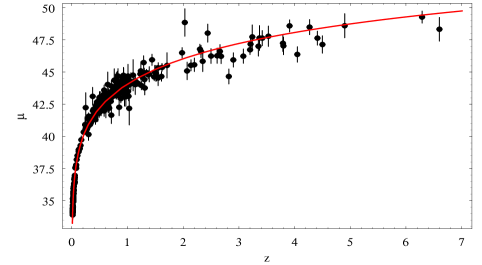
Figure 1: Comparison among predicted and observed SNeIa and GRBs Hubble diagram.

$$\chi^{2}_{SNeIa}=\sum_{i=1}^{{\cal{N}}_{SNeIa}}{\left[\frac{\mu_{obs}(z_{i})-\mu_{th}(z_{i},w_{eff},h)}{\sigma_{i}}\right]^{2}}\ ,\$$ (36)

$$\chi^{2}_{GRB}=\sum_{i=1}^{{\cal{N}}_{GRB}}{\left[\frac{\mu_{obs}(z_{i})-\mu_{th}(z_{i},w_{eff},h)}{\sigma_{i}}\right]^{2}}\ .\$$ (37)

The $\chi^{2}$ terms in (35) take care of the Hubble diagram of SNeIa and GRBs, respectively, and rely on the distance modulus defined as

$$\mu_{th}(z,w_{eff},h)=25+5\log{D_{L}(z,w_{eff},h)}\ .\$$ (38)

We use the Union union dataset for SNeIa and the GRBs sample assembled in Cardone et al. ccd09 to set the observed quantities $(\mu_{obs},\sigma_{i})$ for the SNeIa and GRBs, respectively. Since the Hubble constant $h$ is degenerate with the (unconstrained) absolute magnitude of a SN, we have added a Gaussian prior on $h$ using the results from the HST Key Project freedman thus setting $(h_{HST},\sigma_{HST})=(0.72,0.08)$.

The best fit model turns out to be

$$(w_{eff},h)=(0.55,0.68)\ ,\$$

giving

$$\chi^{2}_{SNeIa}/d.o.f.=1.08\ ,\ \ \chi^{2}_{GRB}/d.o.f.=2.07\ ,\$$

where $d.o.f.=N_{SNeIa}+N_{GRB}-N_{p}$ is the number of degree of freedom of the model, with $N_{SNeIa}=307$ the number of SNeIa in the Union sample, $N_{GRB}=69$ the number of GRBs, and $N_{p}=2$ the number of parameters of the Rastall’s model. While for SNeIa we get a very good reduced $\chi^{2}$, this is not the case for GRBs so that one could be tempted to deem as unsuccessfull the fit. Actually, Fig. 1 shows that the model is indeed fitting quite well both the SNeIa and GRB data so that the large value of $\chi^{2}_{GRB}/d.o.f.$ should be imputed to the large scatter of the high redshift data around the best fit line, not taken into account by the statistical error on the GRBs distance modulus. In order to further test the model, one can consider the constraints on the matter density parameter. Since our model only contains matter, one could naively think that $\Omega_{M}=1$. Actually, one must also take into account that $\Omega_{M}$ is defined using the GR coupling constant $\kappa_{GR}$ which is related to the Rastall’s coupuling $\kappa_{r}$ through Eq.(15). It is then a matter of algebra to show that $\Omega_{M}=w_{eff}$ so that, after marginalizing over $h$, we get the following constraints:

$$\Omega_{M}=0.55_{-0.03\ -0.05}^{+0.02\ +0.05}\ ,$$

where we have used the notation $x^{+x_{1}+x_{2}}_{-y_{1}-y_{2}}$ to mean that $x$ is the median value of the parameter and $(x+x_{1},x-y_{1}),(x+x_{2},x-y_{2})$ are the 68% and 95% confidence ranges respectively. Note that the value thus obtained is in strong disagreement with the typical $\Omega_{M}\simeq 0.3$ obtained from both the cosmic microwave background radiation data and cluster gas mass fractions. Such a large matter density parameter is clearly unacceptable and represents a strong evidence against the Rastall’s model. It is worth noting that such a result could be qualitatively foreseen considering that, because of the non-conservativity of the matter stress-energy tensor, a sort of matter creation takes place thus increasing $\Omega_{M}$ and leading to the final disagreement.
Inverting the relation between $\Omega_{M}$ and $\kappa_{r}\lambda$, we get $\kappa_{r}\lambda=(1-\Omega_{M})/(3-4\Omega_{M})$ so that, for $\Omega_{M}\simeq 0.3$, we get $\kappa_{r}\lambda\simeq 0.39>1/4$. Indeed, our best fit value for $w_{eff}$ gives back a value for $\kappa_{r}\lambda$ that falls outside the suitable range to reproduce an accelerated behaviour.

V Conclusions

In this paper we have focused on Rastall’s theory of gravity, which has been initially motivated by the need for a theory able to allow a non conservativity of the source stress-energy tensor without violating the Bianchi identities. In particular, we have reexamined this model of gravity to investigate the possibility that it could reproduce the observed cosmic speed up. First, we have explicitly worked out the modified Friedmann equations and we have shown that Cardassian-like modifications of Friedmann equations are obtained in Rastall’s model but, contrary to recent claims, they cannot contain time-dependent parameters. Then, we have confronted the model predictions with the available data concerning type Ia Supernovae (SNeIa) and Gamma Ray Bursts (GRBs): what we have showed is that it is possible to get an accelerated expansion that is in agreement with the Hubble diagram of both SNeIa and GRBs, even if there is unfortunately no possibility to reproduce an accelerated-decelerated-accelerated expansion for our universe as it seems to be requested. These results have also a major drawback: indeed, to get them it is necessary to postulate a matter density parameter much larger than the typical $\Omega_{M}\simeq 0.3$ value inferred from cluster gas mass fraction data. As a consequence, Rastall’s theory is not in agreement with current cosmological observations of late time acceleration. However, since the non-conservativity of the matter stress-energy tensor can be related to matter creation, such a model could have important effects during the inflationary period, as it has been suggested smalley93 , even though an analysis of this issue is beyond the scopes of the present paper.

Note added. After the publication of a preprint of this paper, the problem of structure formation in Rastall’s theory has been studied in batista , where the authors point out the difficulties of finding an agreement between this modified gravity model and the observational data.

References

- (1) Riess, A.G., et al., Astron. J. 116, 1009 (1998)
- (2) Perlmutter, S., et al., Astrophys. J. 517, 565 (1999)
- Bennet et al. (2003) Bennet, C.L., et al., Astrophys. J. Suppl. 148, 1 (2003)
- (4) Will, C.M., Living Rev. Relativity 9, http://www.livingreviews.org/lrr-2006-3, (2006)
- (5) Peebles, P.J., Ratra, B., Rev. Mod. Phys. 75, 559 (2003)
- (6) Kamionkowski, M., arXiv:0706.2986 [astro-ph] (2007)
- (7) Kolb, E.W., Matarrese, S., Riotto, A. New J. Phys. 8, 322 (2006)
- (8) Rastall, P., Phys. Rev. D 6, 3357 (1972)
- (9) Smalley, L. L., Class. Quantum Grav. 10, 1179 (1993)
- (10) Lindblom, L., Hiscock, W.A., J. Phys. A 15, 1827 (1982)
- (11) Al - Rawaf, A.S., Mod. Phys. Lett. A 23, 2691 (2008)
- (12) Freese, K., Lewis, M., Phys. Lett. B 540, 1 (2002)
- (13) Fay, S., Amarzguioui, M., Astronomy and Astrophysics 460, 37 (2006)
- (14) Trautman, A., in Lectures on General Relativity, edited by Deser, S., and Ford, K.W., Prentice-Hall, Englewood Cliffs, New Jersey (1965)
- (15) Weinberg, S., Gravitation and Cosmology, J. Wiley and Sons, New York (1972)
- (16) Ferraris, M., Francaviglia, M., Volovich, I., Class. Quant. Grav. 11, 1505 (1994)
- (17) Kowalski M., et al., Astrophys. J. 686, 749 (2008)
- (18) Cardone, V.F., Capozziello, S., Dainotti, M.G., arXiv:0901.3194 [astro-ph.CO] (2009)
- (19) Freedman, W.L. et al., Astrophys. J. 553, 47 (2001)
- (20) Batista, C.E.M., Fabris, J.C., Hamani Daouda, M., arXiv:1004.4603 [astro-ph.CO] (2010)