Dark Periods in Rabi Oscillations of Superconducting Phase Qubit Coupled to a Microscopic Two-Level System

Abstract

We propose a scheme to demonstrate macroscopic quantum jumps in a superconducting phase qubit coupled to a microscopic two-level system in the Josephson tunnel junction. Irradiated with suitable microwaves, the Rabi oscillations of the qubit exhibit signatures of quantum jumps: a random telegraph signal with long intervals of intense macroscopic quantum tunneling events (bright periods) interrupted by the complete absence of tunneling events (dark periods). An analytical model is developed to describe the width of the dark periods quantitatively. The numerical simulations indicate that our analytical model can capture underlying physics of the system. Besides calibrating the quality of the microscopic two-level system, our results have significance in quantum information process since dark periods in Rabi oscillations are also responsible for errors in quantum computing with superconducting qubits.

I INTRODUCTION

Superconducting Josephson devices coherently driven by external fields provide new insights into fundamentals of quantum mechanics and hold promise for use in quantum computation and quantum information.Mooij ; Makhlin ; Nielsen Recent experiments based on Josephson tunnel junctions have unambiguously demonstrated the quantum behavior of macroscopic variable. Jackel ; Nakamura ; Yu ; Martinis One interesting quantum phenomenon is known as quantum jumps, which was proposed by Bohr as early as 1913.Bohr Bohr suggested that the interaction of light and matter occurs in such a way that an atom undergoes instantaneous transitions of its internal state upon the emission or absorption of a light quantum. These sudden transitions have become known as ’quantum jumps’.Scully ; Orszag ; Carmichael ; Plenio ; Blatt Quantum jumps were firstly observed in experiments in the 1980s by investigating the fluorescence of a single trapped ion driven by laser.ion In such atomic systems, quantum jumps are a random telegraphic process with long intervals of intense photon emissions interrupted by periods of the absence of photons. To observe quantum jumps in macroscopic systems such as superconducting qubits, one may naturally think that it can be achieved by detecting microwave photon emissions in analogy with the way in atomic systems. However, this idea suffers from the absence of microwave photodetectors, although some theoretical efforts have been made.Helmer ; Romero Recently, macroscopic quantum jumps were experimentally demonstrated for the first time in a superconducting phase qubit coupled with a TLS inside the Josephson junction.Yu2 In this experiment, the state of the system is read out not by detecting photon emissions but by detecting macroscopic quantum tunneling events, and quantum jumps behave in the form of jumping randomly between upper branch and lower branch of the switching currents. In addition, recent experiments on superconducting charge qubits also demonstrated quantum jumps by observing quasiparticle tunneling in the time domain,Aumentado ; Shaw and theory for the kinetics of the system has been developed.Lut

In this article, we show that macroscopic quantum jumps can be better observed in a Rabi-oscillation experiment in the phase qubit-TLS coupling system. The main points we are going to make are the following. Firstly, quantum jumps in coherent excitations of macroscopic quantum states can be well studied based on our model. In the experiment by Yu et al.,Yu2 the energy level structure keeps changing during the measurement time, and coherent characteristic of the dynamics cannot be observed directly. The scheme proposed in this article is based on a fixed energy level structure, which is usually implemented to demonstrate Rabi oscillations as the basic skill to manipulate quantum states. As we can see below, as a result of the coherent dynamics in our model, some new features of quantum jumps which have not been expected in the previous experiments can appear.

Secondly, macroscopic quantum jumps in the qubit-TLS coupling system bring new insights into our understanding of the effects of TLS on the dynamics of the qubit. Qubit-TLS coupling system has received dramatic attention recently in both experimentalSimmonds ; Kim ; Lup and theoreticalShnirman ; Faoro ; Clare1 ; Galperin ; Clare2 ; Ashhab studies because it is suggested that TLS is a major source of decoherence in superconducting Josephson qubits. In particular, Rabi oscillations in such qubit-TLS coupling system have been studied by several authors. Simmonds ; Galperin ; Clare2 ; Ashhab However, the previous works mainly emphasized on the ensemble characteristic of the system, without considering the effects of quantum jumps in single trajectories, which is actually the original form of experimental data.Yu ; Yu2 Therefore, a detailed description of the effect of TLS on the trajectories of a single qubit is desirable.

Thirdly, recent experiments have demonstrated that TLS can be used as quantum memory with good performance.Neeley It is also suggested that such TLSs themselves can serve as qubits Zagoskin ; LinTian and can be implemented to generate genuine multi-qubit entangled states.Zhu Therefore, characterizing the TLS is critical to improve the performance of such solid-state qubits. In this article, we show that the macroscopic quantum jumps phenomenon can be used to read out the state of TLS, which provides a new approach to calibrate individual TLS quantitatively.

This article is organized as follows. In Sec. II we briefly describe the basic physics of superconducting phase qubit under coherent driving fields, and then introduce the Monte Carlo wavefunction method which can be adopted to study the Rabi oscillations in the superconducting phase qubit. In Sec. III we introduce the qubit-TLS coupling system, and present the Hamiltonian of the hybrid system. In Sec. IV, we provide a clear physical picture of macroscopic quantum jumps in such qubit-TLS coupling system. In Sec. V, we study the width of dark periods in Rabi oscillations quantitatively with both numerical and analytical methods. In Sec VI, we show that the quantum jumps approach can be used to characterize the TLS quantitatively, and this article ends with a brief discussion on the relation between quantum jumps and readout fidelity in superconducting quantum computing.

II QUANTUM JUMP APPROACH TO RABI OSCILLATIONS IN SUPERCONDUCTING PHASE QUBIT

In this section we briefly present the basic physics of superconducting Josephson phase qubit driven by coherent fields, and then introduce how the quantum-jump approach can be used to simulate Rabi oscillations of a single qubit. To grasp the spirit of quantum-jump approach in a simple way, here we firstly consider the qubit without coupling to a TLS.

Superconducting Josephson phase qubit is essentially a current-biased Josephson junction. The Hamiltonian of the phase qubit as shown in Fig.1(a) readsLeggett ; Martinis2 ; Clarke ; Martinis3

$$H_{qb}=\frac{1}{2C}\hat{Q}^{2}-\frac{I_{0}\Phi_{0}}{2\pi}\cos\hat{\delta}-\frac{I\Phi_{0}}{2\pi}\hat{\delta},$$ (1)

where $I_{0}$ is the critical current of the Josephson junction, $I$ is the bias current, $C$ is the junction capacitance, $\Phi_{0}=h/2e$ is the flux quantum, $\hat{Q}$ denotes the charge operator and $\hat{\delta}$ represents the gauge invariant phase difference across the junction, which obeys the convectional quantum commutation relation $[\hat{\delta},\hat{Q}]=2ei$. Quantum behavior can be observed for large area junctions when the bias current is slightly smaller than the critical current. The junction works as a phase qubit when the Josephson coupling energy $E_{J}=I_{0}\Phi_{0}/2\pi$ is much larger than the single charging energy $E_{C}=e^{2}/2C$. In this regime, the two lowest energy levels, $|0\rangle$ and $|1\rangle$ as shown in Fig.1(b), are usually employed as a qubit in quantum computation. The state of the qubit can be controlled through the bias current $I(t)$ given byMartinis3

$$I(t)=I_{dc}+\Delta I(t)=I_{dc}+I_{\mu w}\cos\omega t,$$ (2)

where the classical bias current is parameterized by the dc current $I_{dc}$ and the ac current with the magnitude $I_{\mu w}$ and frequency $\omega$.

Truncating the full Hilbert space of the junction to the qubit subspace $\{|0\rangle$, $|1\rangle\}$, the Hamiltonian of the phase qubit can be written as

$$H_{qb}=\hbar\omega_{0}|0\rangle\langle 0|+\hbar\omega_{1}|1\rangle\langle 1|+\hbar\Omega_{m}\cos\omega t(|0\rangle\langle 1|+|1\rangle\langle 0|),$$ (3)

where $\omega_{n}$ is the energy frequency of state $|n\rangle$, $\Omega_{m}=I_{\mu w}\sqrt{1/2\hbar\omega_{10}C}$ is Rabi frequency, and $\omega_{10}=\omega_{1}-\omega_{0}$ is the energy frequency between state $|0\rangle$ and $|1\rangle$. In the interaction picture and choosing a rotating frame of the frequency $\omega$, Hamiltonian (3) can be simplified to

$$H_{qb}=\hbar\Delta|1\rangle\langle 1|+\frac{\hbar\Omega_{m}}{2}(|0\rangle\langle 1|+|1\rangle\langle 0|),$$ (4)

where $\Delta\equiv\omega_{10}-\omega$ represents the detuning.

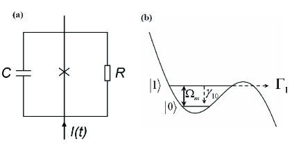
Figure 1: (a) Equivalent circuit of a current-biased Josephson tunnel junction. (b) An illustration of various coherent and incoherent processes in a superconducting phase qubit radiated by a microwave.

To better understand our simulation method, we give a brief description of the experimental procedure firstly. In experiments,Yu the system is prepared in the initial state $|0\rangle$ firstly, then a microwave source is turned on for a duration time $\tau_{m}$ (For convenience, we call $\tau_{m}$ the measurement time below). Because the tunneling rates depend exponentially on the barrier height, the bias current $I_{dc}$ can be chosen so that the tunneling from $|0\rangle$ is essentially ’frozen out’.Yu Therefore, the Rabi oscillations between states $|0\rangle$ and $|1\rangle$ lead to an oscillating probability for the system to tunnel out of the potential. At the end of the measurement time $\tau_{m}$ for a single run, no matter the tunneling event has happened or not, the biased current $I_{dc}$ is adjusted to initialize the state for the next run. Here we label the time interval for initializing the qubit state as $\tau_{p}$.

To simulate the dynamics of the phase qubit system with and without TLS coupling, we adopt Monte Carlo wavefunction method, which is also called ’quantum trajectories’ methodScully ; Orszag ; Carmichael ; Plenio ; Dalibard ; Dalibard2 ; Carmichael2 . In this method, the time evolution of the system can be described by the non-Hermitian effective Hamiltonian

$$H_{eff}=H_{qb}-\frac{i\hbar}{2}(\gamma_{10}+\Gamma_{1})|1\rangle\langle 1|,$$ (5)

where $\gamma_{10}$ is the rate of energy relaxation from $|1\rangle$ to $|0\rangle$ and $\Gamma_{1}$ is the tunneling rate from the level $|1\rangle$ out of the potential. The ’conditional state’ $|\Psi_{c}(t)\rangle$ of the system is determined by

$$|\Psi_{c}(t+\delta t)\rangle=\exp[-iH_{eff}\delta t/\hbar]|\Psi_{c}(t)\rangle.$$ (6)

The procedure adopted in quantum-jump simulation of Rabi oscillations of a single qubit can be summarized as follows:

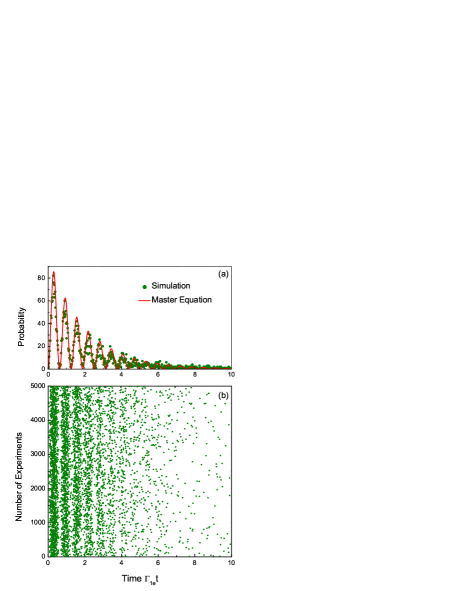
Figure 2: (Color online)Simulated Rabi oscillations of a single superconducting phase qubit. (a) Average over $N=5000$ quantum tunneling events obtained using Monte Carlo wavefunction method(green dots). The red line is an ensemble result obtained using master equation. (b) Trajectories of quantum tunneling events obtained with Monte Carlo wavefunction method. The parameters are $\Omega_{m}=10\Gamma_{1}$, $\Delta=0$, and $\gamma_{10}=\Gamma_{1}/4$.

(i) Determine the current probability of a relaxation or tunneling event, i.e., $\Delta P_{r}=\gamma_{10}\delta t\langle\Psi|1\rangle\langle 1|\Psi\rangle$ and $\Delta P_{t}=\Gamma_{1}\delta t\langle\Psi|1\rangle\langle 1|\Psi\rangle$.

(ii) Obtain random numbers $r_{1}$ and $r_{2}$ between zero and one, compare with $\Delta P_{t}$ and $\Delta P_{r}$ respectively, and decide on tunneling or relaxation for different cases:

(a) If $r_{1}<\Delta P_{t}$ a quantum tunneling event happens. Register the time $t$ of the event, and then turn to step (iii).

(b) If $r_{1}>\Delta P_{t}$ and $r_{2}<\Delta P_{t}$ there is a relaxation, so that the system jumps to the state $|0\rangle$.

(c) If $r_{1}>\Delta P_{r}$ and $r_{2}>\Delta P_{t}$ no quantum jumps take place, so the system evolves under the influence of the non-Hermitian form

$$|\Psi\rangle\to\frac{\{1-(i/\hbar)H_{qb}\delta t-(\gamma/2)\delta t|1\rangle\langle 1|\}|\Psi\rangle}{(1-\Delta P)^{1/2}},$$ (7)

where $\gamma\equiv\gamma_{10}+\Gamma_{1}$ and $\Delta P\equiv\Delta P_{r}+\Delta P_{t}$.

(iii) If no tunneling event happens, repeat the previous steps until the end of the measurement time $\tau_{m}$.

(iv) Accounting time $t$ over many simulation runs.

By using this Monte Carlo wavefunction method, we simulate the trajectories of Rabi oscillations in a single superconducting phase qubit and the results are shown in Fig.2(b). We emphasize that it is possible that a tunneling event never happens during a finite measurement time $\tau_{m}$ for a single run, which is important for observing dark periods as discussed in Sec. V. To test the efficiency of our simulation method, we compare the simulated results with those obtained with master equation used in Ref [6]. As shown in Fig.2(a), they agreed very well. Actually, it can be proved that the Monte Carlo method is equivalent, on average, to the master equation.Scully ; Orszag ; Carmichael Guaranteed with the efficient method for simulating Rabi oscillations in superconducting phase qubit, we turn to the more interesting qubit-TLS coupling system.

III HAMILTONIAN OF QUBIT-TLS COUPLING SYSTEM

Experiments have shown that some TLSs may locate inside the Josephson tunnel barrier, as illustrated in Fig.3(a). A TLS is understood to be an atom, or a small group of atoms, that tunnels between two lattice configurations, Phillips ; Neeley , with different wave functions $|L\rangle$ and $|R\rangle$. The two states of the TLS correspond to two different values of the Josephson junction critical current $I_{0}$ which is proportional to the square of the tunneling matrix element across the junction. When the TLS is in state $|R\rangle$ ($|L\rangle$), the junction critical current is $I_{0R}$ ($I_{0L}$). Then the interaction Hamiltonian between the qubit and the TLS is:

$$H_{int}=-\frac{\Phi_{0}I_{0R}}{2\pi}\cos\delta\otimes|R\rangle\langle R|-\frac{\Phi_{0}I_{0L}}{2\pi}\cos\delta\otimes|L\rangle\langle L|.$$ (8)

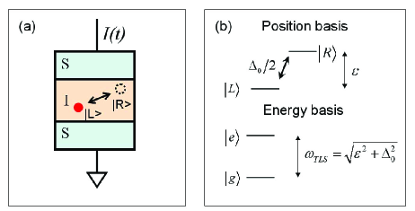
Figure 3: (Color online) (a) Schematic of a TLS in the oxide tunnel barrier of the Josephson junction. Because the barrier material is disordered, some atoms can occupy two positions, labelled $|L\rangle$ and $|R\rangle$. (b) The position states are separated by an energy difference $\varepsilon$ and connected by a tunneling energy $\Delta_{0}/2$. In the energy eigenstate basis, the ground state $|g\rangle$ and excited state $|e\rangle$, are separated by an energy $\omega_{TLS}$. The charge motion between $|L\rangle$ and $|R\rangle$ couples to the currents and voltages of the qubit circuit.

Assume an asymmetric potential with energy separated by $\hbar\omega_{TLS}$ for the TLS, then the ground and excited states are $|g\rangle=\sin(\theta/2)|L\rangle+\cos(\theta/2)|R\rangle$ and $|e\rangle=\cos(\theta/2)|L\rangle-\sin(\theta/2)|R\rangle$, where $\omega_{TLS}=\sqrt{\varepsilon^{2}+\Delta_{0}^{2}}$, $\theta=\arctan(\Delta_{0}/\varepsilon)$ with $\varepsilon/2$ being the energy asymmetry and $\Delta_{0}/2$ being the bare tunneling matrix element (Fig.3(b)). Considering the junction is biased near its critical currentMartinis3 ; Clare2 , i.e., $\delta=\pi/2-\delta^{\prime}$ with $|\delta^{\prime}|\ll 1$, then $\cos(\pi/2-\delta^{\prime})=\sin\delta^{\prime}\approx\delta^{\prime}$. In this case, $\delta^{\prime}$ can be well approximated as position coordinate operator of the harmonic oscillator. Using these facts and including only the dominant resonant terms arising from the interaction Hamiltonian, Equation (8) becomes

$$H_{int}=\frac{\delta I_{0}\sin\theta}{2}\sqrt{\frac{\hbar}{2\omega_{10}C}}(|0e\rangle\langle 1g|+|1g\rangle\langle 0e|),$$ (9)

where $\delta I_{0}\equiv I_{0R}-I_{0L}$ is the fluctuation amplitude in $I_{0}$ produced by the TLS. The coupling of the two intermediate energy levels through $H_{int}$ produces an energy splitting which can be characterized in spectroscopic measurements.Yu2 ; Simmonds ; Kim ; Lup The Hamiltonian of the qubit-TLS coupling system in the basis {$|0g\rangle$, $|1g\rangle$, $|0e\rangle$, and $|1e\rangle$} then reads

$$H=\hbar\left(\begin{array}[]{cccc}0&\Omega_{m}\cos\omega t&0&0\\ \Omega_{m}\cos\omega t&\omega_{10}&\Omega_{c}&0\\ 0&\Omega_{c}&\omega_{TLS}&\Omega_{m}\cos\omega t\\ 0&0&\Omega_{m}\cos\omega t&\omega_{10}+\omega_{TLS}\\ \end{array}\right).$$ (10)

To understand the underlying physics that governs the dynamic of the system more clearly, we chose the interaction picture and make a transformation to a rotating frame. Then the Hamiltonian can be simplified to the time independent form (see appendix)

$$H^{\prime}=\hbar\left(\begin{array}[]{cccc}0&\Omega_{m}/2&0&0\\ \Omega_{m}/2&\Delta&\Omega_{c}&0\\ 0&\Omega_{c}&\Delta+\Delta_{r}&\Omega_{m}/2\\ 0&0&\Omega_{m}/2&2\Delta+\Delta_{r}\\ \end{array}\right),$$ (11)

where $\Delta\equiv\omega_{10}-\omega$ and $\Delta_{r}\equiv\omega_{TLS}-\omega_{10}$ are the detunings, $\Omega_{c}=(\delta I_{0}\sin\theta/2)\sqrt{1/(2\hbar\omega_{10}C)}$ i s the avoided energy level crossing between $|0e\rangle$ and $|1g\rangle$, and $\Omega_{m}=I_{\mu w}\sqrt{1/2\hbar\omega_{10}C}$ is the Rabi frequency between the qubit state $|0\rangle$ and $|1\rangle$. From Hamiltonian (11), we can divide the system into two subspaces $A\equiv\{|0g\rangle,|1g\rangle\}$ and $B\equiv\{|0e\rangle,|1e\rangle\}$. The effective coupling strength between $A$ and $B$ is decided by several parameters including $\Omega_{c}$, $\Delta_{r}$, $\Delta$ and $\Omega_{m}$. Interestingly, the parameters $\Delta_{r}$, $\Delta$ and $\Omega_{m}$ can be easily controlled by adjusting the bias current $I_{dc}$, the microwave frequency and the microwave amplitude, respectively.Yu2 While in the interior of the subsystem, the coupling strength $\Omega_{m}/2$ between states $|0g\rangle$ and $|1g\rangle$ ($|0e\rangle$ and $|1e\rangle$ ) can be controlled by adjusting the amplitude of the microwave.Yu ; Martinis Therefore, the qubit-TLS coupling system behaves as an ”artificial atom” which can be manipulated flexibly.

IV QUANTUM JUMPS IN QUBIT-TLS COUPLING SYSTEM

To have a clear physical picture of macroscopic quantum jumps in qubit-TLS coupling system, we provide an analogy with quantum jumps in quantum optics, which has been well developed for years. Scully ; Orszag ; Carmichael ; Plenio ; Blatt ; ion ; Dalibard ; Dalibard2 ; Carmichael2 In quantum optics, the system generally has energy structure shown in Fig.4(a). Two excited states $|1\rangle$ and $|2\rangle$ are connected to a common ground state $|0\rangle$ via a strong and weak transition, respectively. The fluorescent photons from the strong transition are observed. However, an excitation of the weak transition where the electron is temporarily shelved in the metastable level $|2\rangle$ will cause the strong transition to be turned off. Therefore, it is possible to monitor the quantum jumps of the weak transition via the signal provided by the fluorescence of the strong transition. In the language of quantum measurement theory,Zurek the fluorescence from the strong transition acts as a pointer from which the microscopic quantum state of the atom may be determined.

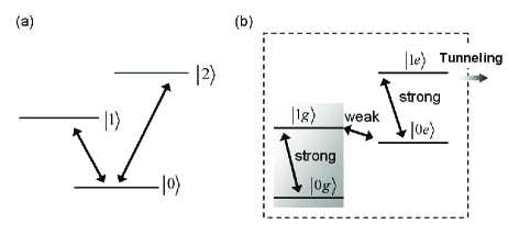
Figure 4: (a) $V$-type energy structure for observing quantum jumps in the fluorescence of a single atom. Two upper levels $|1\rangle$ and $|2\rangle$ couple to a common ground state $|0\rangle$. The $|1\rangle\leftrightarrow|0\rangle$ transition is assumed to be strong while the $|2\rangle\leftrightarrow|0\rangle$ transition is weak. (b) Schematic energy level diagram for a junction coupled to a TLS. The ground state (the excited state) of the qubit is denoted as $|0\rangle$ ($|1\rangle$); $|g\rangle$ and $|e\rangle$ represent the ground state and the excited state of TLS. The $|1g\rangle\leftrightarrow|0e\rangle$ transition is weak, while the $|0e\rangle\leftrightarrow|1e\rangle$($|0g\rangle\leftrightarrow|1g\rangle$) transition is strong.

Similarly, in the qubit-TLS coupling system considered here, quantum jumps between macroscopic quantum states are also proposed to happen. As discussed in Sec. III, we can have a weak transition between states $|1g\rangle$ and $|0e\rangle$ by adjusting the bias current and a strong transition between $|0e\rangle$ and $|1e\rangle$(or between $|0g\rangle$ and $|1g\rangle$) by adjusting the microwave amplitude. However, different from observing fluorescent photons in atom systems, the states of the qubit-TLS coupling system are read out through quantum tunneling. As has been proved in experiments Yu2 , in the qubit-TLS coupling system, different states correspond to different tunneling rates.reason1 Therefore, by adjusting the bias current at a proper value, only the tunneling from state $|1e\rangle$ is prominent, and tunneling from other states can be neglected.

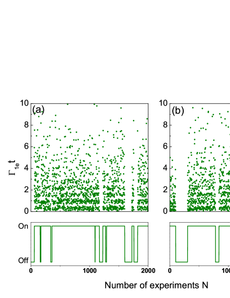
Figure 5: (Color online) Dark periods in Rabi oscillations of qubit-TLS coupling system. The detunings are (a) $\Delta_{r}=2\Gamma_{1e}$ and (b) $\Delta_{r}=5\Gamma_{1e}$. Lower panel: the filtered data corresponds to on and off of the Rabi oscillations. The parameters for simulation are $\Delta=0$, $\gamma_{10}=\Gamma_{1e}/4$, $\Omega_{c}=\Gamma_{1e}/4$, $\Omega_{m}=10\Gamma_{1e}$, and $\tau_{m}=10/\Gamma_{1e}$.

Then the physics for quantum jumps in qubit-TLS coupling system is straightforward. When the system stays in subspace $B\{|0e\rangle,|1e\rangle\}$, quantum tunneling events in the Rabi oscillation form (see Fig.2) can be observed. However, once the system transitions into subspace $A\{|0g\rangle,|1g\rangle\}$ (dark area in Fig.4(b)), where the system has little probability to tunnel out the potential, no quantum tunneling events can be observed during the measurement time, and then dark periods in Rabi oscillations appear. To substantiate our proposal, we investigate this phenomena numerically with the Monte Carlo wavefunction method introduced in Sec. II. In the qubit-TLS coupling system, the dynamics can be described by the non-Hermitian effective Hamiltonian

$$H_{eff}=H^{\prime}-\frac{i\hbar}{2}(\gamma_{10}+\Gamma_{1e})|1e\rangle\langle 1e|-\frac{i\hbar}{2}\gamma_{10}|1g\rangle\langle 1g|,$$ (12)

where $\Gamma_{1e}$ is the tunneling rate of state $|1e\rangle$ and $\gamma_{10}$ is the relaxation rate from $|1e\rangle$ to $|0e\rangle$ ($|1g\rangle$ to $|0g\rangle$). It is noticed that we do not take into account the relaxation effect of the TLS, because the lifetime of the TLS is much longer than that of the phase qubit.Zhu ; Zagoskin ; Simmonds Actually, this effect can be easily considered in the same way as we consider the relaxation of the qubit. The quantum state either evolves according to the schrödinger equation, or ’jumps’ to an eigenstate of the system with certain probability. The measurement result serves as a pointer to determine the quantum state of the system. Once a quantum tunneling event happens, we know that the state of TLS is $|e\rangle$; then in the next run the initial state of the system is prepared in the corresponding qubit ground state $|0e\rangle$. On the contrary, if no quantum tunneling event happens during a sufficient long measurement time $\tau_{m}$, we can confirm that the system is in subspace $A\{|0g\rangle,|1g\rangle\}$, i.e., the state of TLS is $|g\rangle$. Then in the next run of simulation the initial state is prepared in the corresponding qubit ground state $|0g\rangle$ and dark periods in Rabi oscillations may appear. We emphasize that if the measurement time $\tau_{m}$ is short, the TLS’s state cannot be determined if no quantum tunneling event happens at the end of $\tau_{m}$. In this case, we decide the initial state of the next run using Monte Carlo method according to the population of $|g\rangle$ and $|e\rangle$ respectively.

As shown in Fig.5, in the simulated trajectories the quantum tunneling events are disturbed by dark periods during which no tunneling events are observed. In addition, it is found that the average width $\langle N_{D}\rangle$ of dark periods for $\Delta_{r}=2\Gamma_{1e}$ is smaller than that for $\Delta_{r}=5\Gamma_{1e}$ (Here $\langle N_{D}\rangle$ means the the average number of runs in a single dark period). One may simply think that as the detuning $\Delta_{r}$ increases, the coupling between subspace $A$ and subspace $B$ becomes weaker. Therefore the system is more difficult to make transitions between $A$ and $B$, thus leading to a larger average width of dark periods. However, this is not always the case. As discussed below, we will give a quantitative description between $\langle N_{D}\rangle$ and $\Delta_{r}$.

V RELATION BETWEEN DARK PERIODS AND DETUNING

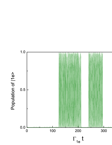
Figure 6: (Color online) The time evolution of the population of state $|1e\rangle$. The dark periods correspond to the shelving of the system in subspace $A\{|0g\rangle,|1g\rangle\}$. The parameters are $\Delta=0$, $\gamma_{10}=\Gamma_{1e}/4$, $\Omega_{c}=\Gamma_{1e}/4$, $\Omega_{m}=10\Gamma_{1e}$, and $\Delta_{r}=2\Gamma_{1e}$

In this section we study the relationship between the average width $\langle N_{D}\rangle$ of dark periods and the detuning $\Delta_{r}$. We start from investigating the transition rate from subspace $A\{|0g\rangle,|1g\rangle\}$ to subspace $B\{|0e\rangle,|1e\rangle\}$, i.e., $\Gamma_{D}=1/T_{D}$, where $T_{D}$ is the lifetime of the dark periods. A simple method is to study the time evolution of the population of $|1e\rangle$ in the qubit-TLS coupling system based on the effective Hamiltonian (12). As shown in Fig.6 (Here we have deducted the initial-state preparing time $\tau_{p}$), the population of $|1e\rangle$ is interrupted by random periods of ’darkness’. Quantum jumps from dark periods to bright periods indicate that the system jumps from subspace $A$ to subspace $B$. We make an ensemble average over the lifetime of the dark periods. As shown in Fig.7, it is interesting that the transition rates reveal three peaks as a function of the detuning $\Delta_{r}$. In addition, we find that the positions for the two side peaks are $\Omega_{m}$ and $-\Omega_{m}$, respectively.

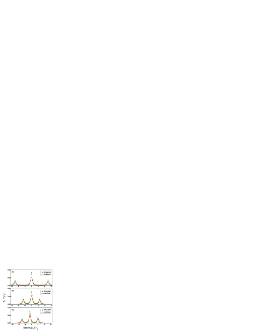
Figure 7: (Color online) Transition rate $1/T_{D}$ versus the detuning $\Delta_{r}$. $T_{D}$ represents the average lifetime of the dark periods as shown in Fig. 6. The red solid lines show the analytical results obtained from Eqs.(14-15) and the green dots show the simulation results. Each green dot is obtained by averaging over $N=4000$ dark periods. The parameters used in both analytical solutions and simulations are: $\gamma_{10}=\Gamma_{1e}/4$, $\Omega_{c}=\Gamma_{1e}/4$, and (a) $\Delta=0$, $\Omega_{m}=10\Gamma_{1e}$, (b) $\Delta=0$, $\Omega_{m}=5\Gamma_{1e}$, (c) $\Delta=1\Gamma_{1e}$, $\Omega_{m}=5\Gamma_{1e}$. The positions of the three peaks are determined by $\Delta_{r}=-\sqrt{\Delta^{2}+\Omega_{m}^{2}}-\Delta$, $-\Delta$ and $\sqrt{\Delta^{2}+\Omega_{m}^{2}}-\Delta$, respectively. It is noticed that the heights of the side peaks are equal for $\Delta=0$ and unequal for $\Delta\neq 0$.

To understand the underlying physics, we rewrite the Hamiltonian (11) in the subspace $A$ and $B$, respectively. In the resonant case $\Delta=0$, the Hamiltonian in the basis $\{|A_{e}\rangle\equiv(|0g\rangle+|1g\rangle)/\sqrt{2},|A_{g}\rangle\equiv(|0g\rangle-|1g\rangle)/\sqrt{2},|B_{e}\rangle\equiv(|0e\rangle+|1e\rangle)/\sqrt{2},|B_{g}\rangle\equiv(|0e\rangle-|1e\rangle)/\sqrt{2}\}$ reads (see appendix)

$$H_{A-B}=\hbar\left(\begin{array}[]{cccc}\Omega_{m}/2&0&\Omega_{c}/2&\Omega_{c}/2\\ 0&-\Omega_{m}/2&-\Omega_{c}/2&-\Omega_{c}/2\\ \Omega_{c}/2&-\Omega_{c}/2&\Delta_{r}+\Omega_{m}/2&0\\ \Omega_{c}/2&-\Omega_{c}/2&0&\Delta_{r}-\Omega_{m}/2\\ \end{array}\right),$$ (13)

from which it is clear that the eigenstates in subspace $A$ can couple to the eigenstates in subspace $B$ independently with the coupling strength $\Omega_{c}/2$. Then the physical picture is clear as follows. The energy separation between the two eigenstates in each subspace is equal to the Rabi frequency $\Omega_{m}$. For the detuning $\Delta_{r}=0$, $|A_{e}\rangle$ is resonant with $|B_{e}\rangle$, and $|A_{g}\rangle$ is resonant with $|B_{g}\rangle$; for $\Delta_{r}=\Omega_{m}$, only $|A_{e}\rangle$ is resonant with $|B_{g}\rangle$; and for $\Delta_{r}=-\Omega_{m}$, only $|A_{g}\rangle$ is resonant with $|B_{e}\rangle$. Note that all coupling strengthes are $\Omega_{c}/2$, one would intuitively expect the height of the central peak to be twice that of a side peak, and it confirms from the results of the simulation. Furthermore, we utilize the Wilcox-Lamb method Lamb to obtain an analytical form of the transition rate $\Gamma_{D}$. In the approximation to the first order, the transition rate from subspace $A$ to subspace $B$ has a simple form

$$\Gamma_{D}=\frac{\Omega_{c}^{2}}{2}\sum_{i\in A,j\in B}\frac{\rho_{i}\gamma}{\Delta_{ij}^{2}+\gamma^{2}},$$ (14)

where $\gamma=(2\gamma_{10}+\Gamma_{1e})/2$, $\rho_{i}$ is the probability of state $|i\rangle$ (here $\rho_{A_{e}}=\rho_{A_{g}}=1/2$), and $\Delta_{ij}$ are the detunings between states $|i\rangle$ ($|i\rangle\in\{|A_{e}\rangle,|A_{g}\rangle\}$) and $|j\rangle$ (($|j\rangle\in\{|B_{e}\rangle,|B_{g}\rangle\}$) in the forms $\Delta_{Ae,Be}=\Delta_{Ag,Bg}=\Delta_{r}$, $\Delta_{Ae,Bg}=\Delta_{r}-\Omega_{m}$, and $\Delta_{Ag,Be}=\Delta_{r}+\Omega_{m}$. As shown in Fig.7(a-b), our approximate analytical results agree with the simulation results considerably.

Furthermore, Equation (14) can be straightforwardly generalized to the off resonant case $\Delta\neq 0$ in the form

$$\Gamma_{D}=2\Omega_{c}^{2}\sum_{i\in A,j\in B}\frac{\rho_{i}\lambda_{ij}^{2}\gamma}{\Delta_{ij}^{2}+\gamma^{2}},$$ (15)

where $\lambda_{ij}$ represent the coupling coefficients between states $|i\rangle$ and $|j\rangle$. Here $|i\rangle\in\{|A_{e}\rangle\equiv\sin\frac{\alpha}{2}|0g\rangle+\cos\frac{\alpha}{2}|1g\rangle,|A_{g}\rangle\equiv\cos\frac{\alpha}{2}|0g\rangle-\sin\frac{\alpha}{2}|1g\rangle\}$, and $|j\rangle\in\{|B_{e}\rangle\equiv\sin\frac{\alpha}{2}|0e\rangle+\cos\frac{\alpha}{2}|1e\rangle,|B_{g}\rangle\equiv\cos\frac{\alpha}{2}|0e\rangle-\sin\frac{\alpha}{2}|1e\rangle\}$ with $\alpha=\arctan(\Omega_{m}/\Delta)$. The coupling coefficients $\lambda_{ij}$ have the forms (see appendix) $\lambda_{Ae,Be}=\sin\frac{\alpha}{2}\cos\frac{\alpha}{2}$, $\lambda_{Ag,Bg}=-\sin\frac{\alpha}{2}\cos\frac{\alpha}{2}$, $\lambda_{Ag,Be}=-\sin^{2}\frac{\alpha}{2}$, and $\lambda_{Ae,Bg}=\cos^{2}\frac{\alpha}{2}$, respectively. The detunings $\Delta_{ij}$ have the forms $\Delta_{Ag,Bg}=\Delta_{Ae,Be}=\Delta_{r}+\Delta$, $\Delta_{Ag,Be}=\Delta_{r}+\Delta+\sqrt{\Omega_{m}^{2}+\Delta^{2}}$, and $\Delta_{Ae,Bg}=\Delta_{r}+\Delta-\sqrt{\Omega_{m}^{2}+\Delta^{2}}$, then the positions of the three peaks are given by $\Delta_{r}=-\sqrt{\Delta^{2}+\Omega_{m}^{2}}-\Delta$, $-\Delta$ and $\sqrt{\Delta^{2}+\Omega_{m}^{2}}-\Delta$, respectively. Conclusively, there are two main differences between the resonance case ($\Delta=0$) and the off resonance case ( $\Delta\neq 0$). Firstly, the positions of the three peaks for $\Delta=0$ are symmetric with respect to $\Delta_{r}=0$ but unsymmetric for $\Delta\neq 0$. Secondly, in the case $\Delta=0$ the heights of the side peaks are equal, because all the coupling coefficients between $|i\rangle$ and $|j\rangle$ have the same value $1/2$. However, in the case $\Delta\neq 0$, the heights of the side peaks are unequal because of the different coupling coefficients $\lambda_{ij}$. As expected, the above analysis is well demonstrated in Fig. 7(b-c), where the agreements between numerical simulations and analytical results are clear.

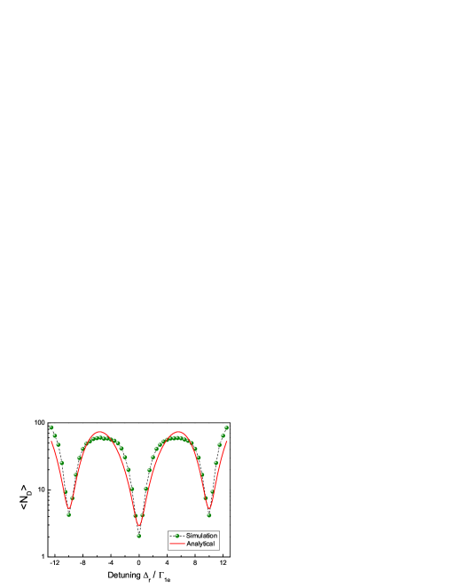
Figure 8: (Color online) Average width $\langle N_{D}\rangle$ of dark periods versus detuning $\Delta_{r}$. The red solid line shows the analytical result obtained from Eq.(14)-Eq.(17), and the green dot shows the simulation result. The parameters used in both analytical solution and simulation are: $\Delta=0$, $\gamma_{10}=\Gamma_{1e}/4$, $\Omega_{c}=\Gamma_{1e}/4$, $\Omega_{m}=10\Gamma_{1e}$ and $\tau_{m}=10/\Gamma_{1e}$.

Then we can estimate the average width $\langle N_{D}\rangle$ of the dark periods in Fig.5. Supposing the system is in subspace $A$ initially, the probability for the system residing in $A$ at the end of a single run with interval $\tau_{m}$ is

$$P=\exp({-\Gamma_{D}\tau_{m}}).$$ (16)

Because the probability $P$ for each run is independent, the average width of the dark periods can be expressed as

$$\langle N_{D}\rangle=\frac{\sum_{n=1}^{\infty}nP^{n}(1-P)}{\sum_{n=1}^{\infty}P^{n}(1-P)}=\frac{1}{1-\exp({-\Gamma_{D}\tau_{m}})}.$$ (17)

Both the simulated and analytical results for $\langle N_{D}\rangle$ are shown in Fig.8 and they agreed very well. The agreement between the numerical and analytical results indicated the validity of our model. In experiments, the coupling strength $\Omega_{c}$ is typically 20MHz $\sim$ 100MHz,Yu2 ; Simmonds ; Neeley $\gamma_{10}$ is typically 1MHz$\sim$100MHz, and other parameters including $\Gamma_{1e}$, $\Delta_{r}$ and $\Omega_{m}$ can be controlled flexibly in a large regime to fulfill our theoretical discussions by manipulating the biased current or microwave amplitude.Yu ; Martinis Therefore, our scheme is feasible within the current technique.

VI CONCLUSION

We have proposed a scheme to observe macroscopic quantum jumps in Rabi oscillations of a superconducting phase qubit coupled to a TLS. This scheme provides a new tool to characterize the TLS quantitatively. Dark periods and bright periods in Rabi oscillations indicate the TLS residing in states $|g\rangle$ and $|e\rangle$, respectively. Therefore, the paramerer $\Gamma_{D}$ discussed in Sec. V describes the transition rate between $|g\rangle$ and $|e\rangle$ of TLS, which is induced by the coupling between qubit and TLS. To obtain the intrinsic lifetime of the TLS, which is known as induced by coupling to elastic strain field,Clare2 we just need to decouple the TLS with qubit by setting the detuning $\Delta_{r}\gg\Omega_{m}$. Moreover, in recent experiments, the TLSs are observed in other kinds of superconducting qubits such as charge qubitAumentado ; Shaw ; Kim and flux qubitLup . We believe that the method and model in this article can also be generalized to such systems as well as other systems with similar energy level structure.

Furthermore, in the process of quantum computing, the quantum computer usually evolves into a highly entangled state. A quantum jump tends to destroy such entangled state and make the result of quantum computing incorrect, which is known as decoherence induced by quantum jumps. However, in this article we found that quantum jumps can lead to another type of negative effect on quantum computing, that is, the errors in reading out the quantum state. For example, once the system jumps into the dark periods, the qubit’s state cannot be read out using the normal methods, although the qubit can still evolve coherently between state $|0\rangle$ and $|1\rangle$. In this case, from the measurement results, we always believe the qubit is staying in state $|0\rangle$. That is to say, quantum jumps leads to a readout error in the qubit. Since the previous literatures emphasized the decoherence induced by the quantum jumps, we hope the discussion in this article can bring new insights into our understanding of the effects of quantum jumps on quantum computing.

VII ACKNOWLEDGMENTS

We thank Clare C. Yu for useful discussions. This work was partially supported by the NSFC (under Contract Nos. 10674062,10725415, and 10674049), the State Key Program for Basic Research of China (under Contract Nos. 2006CB921801 and 2007CB925204), and the Doctoral Funds of the Ministry of Education of the People s Republic of China (under Contract No. 20060284022 ).

VIII APPENDIX: DERIVATION OF EQ.(11) and EQ.(13)

In this appendix, we address the derivation of Eqs. (11) and (13). Under the interaction picture and the rotating wave approximation, the Hamiltonian (10) becomes

$$\hat{H}_{I}=\hbar\left(\begin{array}[]{cccc}0&\Omega_{m}e^{-i\Delta t}/2&0&0\\ \Omega_{m}e^{i\Delta t}/2&0&\Omega_{c}e^{-i\Delta_{r}t}&0\\ 0&\Omega_{c}e^{i\Delta_{r}t}&0&\Omega_{m}e^{-i\Delta t}/2\\ 0&0&\Omega_{m}e^{i\Delta t}/2&0\\ \end{array}\right),$$ (18)

where $\Delta\equiv\omega_{10}-\omega$ and $\Delta_{r}\equiv\omega_{TLS}-\omega_{10}$ are the detunings. We make a transformation to the rotating frame such that the wave function $|\psi\rangle$ in the original Hamiltonian (18) can be expressed as

$$|\psi\rangle=\hat{U}(t)|\psi^{\prime}\rangle,$$ (19)

where

$$\hat{U}(t)=\left(\begin{array}[]{cccc}1&0&0&0\\ 0&e^{i\Delta t}&0&0\\ 0&0&e^{i(\Delta+\Delta_{r})t}&0\\ 0&0&0&e^{i(2\Delta+\Delta_{r})t}\\ \end{array}\right).$$ (20)

Then the Schr$\ddot{o}$dinger equation

$$i\hbar\frac{\partial}{\partial t}|\psi\rangle=\hat{H}_{I}|\psi\rangle,$$ (21)

can now be rewritten as

$$i\hbar\frac{\partial}{\partial t}|\psi^{\prime}\rangle=\hat{H}^{\prime}|\psi^{\prime}\rangle,$$ (22)

where

$$\hat{H}^{\prime}= \hat{U}^{\dagger}(t)\hat{H}_{I}\hat{U}(t)-i\hbar\hat{U}^{\dagger}(t)\frac{d\hat{U}(t)}{dt}$$

$$= \hbar\left(\begin{array}[]{cccc}0&\Omega_{m}/2&0&0\\ \Omega_{m}/2&\Delta&\Omega_{c}&0\\ 0&\Omega_{c}&\Delta+\Delta_{r}&\Omega_{m}/2\\ 0&0&\Omega_{m}/2&2\Delta+\Delta_{r}\\ \end{array}\right).$$ (27)

This transformed Hamiltonian is exactly Eq.(11). To understand the relationship between the lifetime of dark periods and detunings as discussed in Sec. V, we rewrite the Hamiltonian $\hat{H}^{\prime}$ in the basis $\{{|A_{e}\rangle,|A_{g}\rangle,|B_{e}\rangle,|B_{g}\rangle}\}$. In this new basis, we find that the Hamiltonian in the resonant case $\Delta=0$ is actually Eq.(13) given by

$$\hat{H}_{A-B}=\hat{V}^{\dagger}\hat{H}^{\prime}\hat{V}$$

$$=\hbar\left(\begin{array}[]{cccc}\Omega_{m}/2&0&\Omega_{c}/2&\Omega_{c}/2\\ 0&-\Omega_{m}/2&-\Omega_{c}/2&-\Omega_{c}/2\\ \Omega_{c}/2&-\Omega_{c}/2&\Delta_{r}+\Omega_{m}/2&0\\ \Omega_{c}/2&-\Omega_{c}/2&0&\Delta_{r}-\Omega_{m}/2\\ \end{array}\right),$$ (33)

where

$$\hat{V}=\frac{1}{\sqrt{2}}\left(\begin{array}[]{cccc}1&1&0&0\\ 1&-1&0&0\\ 0&0&1&1\\ 0&0&1&-1\\ \end{array}\right).$$ (35)

For the general off resonance case $\Delta\neq 0$, we have

$$\hat{H}_{A-B}=\hat{V}^{\dagger}\hat{H}^{\prime}\hat{V}$$

$$=\hbar\left(\begin{array}[]{cccc}\omega_{Ae}&0&\lambda_{Ae,Be}\Omega_{c}&\lambda_{Ae,Bg}\Omega_{c}\\ 0&\omega_{Ag}&\lambda_{Ag,Be}\Omega_{c}&\lambda_{Ag,Bg}\Omega_{c}\\ \lambda_{Ae,Be}\Omega_{c}&\lambda_{Ag,Be}\Omega_{c}&\omega_{Be}&0\\ \lambda_{Ae,Bg}\Omega_{c}&\lambda_{Ag,Bg}\Omega_{c}&0&\omega_{Bg}\\ \end{array}\right),$$ (40)

where $\omega_{Ae}=(\Delta+\sqrt{\Omega_{m}^{2}+\Delta^{2}})/2$, $\omega_{Ag}=(\Delta-\sqrt{\Omega_{m}^{2}+\Delta^{2}})/2$, $\omega_{Be}=(\Delta+\sqrt{\Omega_{m}^{2}+\Delta^{2}})/2+\Delta+\Delta_{r}$, $\omega_{Bg}=(\Delta-\sqrt{\Omega_{m}^{2}+\Delta^{2}})/2+\Delta+\Delta_{r}$, $\lambda_{Ae,Be}=\sin\frac{\alpha}{2}\cos\frac{\alpha}{2}$, $\lambda_{Ae,Bg}=\cos^{2}\frac{\alpha}{2}$, $\lambda_{Ag,Be}=-\sin^{2}\frac{\alpha}{2}$, $\lambda_{Ag,Bg}=-\sin\frac{\alpha}{2}\cos\frac{\alpha}{2}$, and

$$\hat{V}=\left(\begin{array}[]{cccc}\sin\frac{\alpha}{2}&\cos\frac{\alpha}{2}&0&0\\ \cos\frac{\alpha}{2}&-\sin\frac{\alpha}{2}&0&0\\ 0&0&\sin\frac{\alpha}{2}&\cos\frac{\alpha}{2}\\ 0&0&\cos\frac{\alpha}{2}&-\sin\frac{\alpha}{2}\\ \end{array}\right),$$ (42)

with $\alpha=\arctan(\Omega_{m}/\Delta)$.

References

- (1) J. E. Mooij, Science 307, 1210 (2005).
- (2) Y. Makhlin, G. Schön, and A. Shnirman, Rev. Mod. Phys 73, 357 (2001).
- (3) M. A. Nielsen and I. L. Chuang, Quantum Computation and Quantum Information(Cambridge Univ. Press, Cambridge, 2000).
- (4) L. D. Jackel, J. P. Gordon, E. L. Hu, R. E. Howard, L. A. Fetter, D. M. Tennant, and R. W. Epworth, Phys. Rev. Lett. 47, 697 (1981); R. F. Voss and R. A. Webb, ibid., 265 (1981); R. H. Koch, D. J. Van Harlingen, and J. Clarke, Phys. Rev. Lett. 47, 1216 (1981); J. Clarke, A. N. Cleland, M. H. Devoret, D. Esteve, and J. M. Martinis, Science 239 992 (1988); J. M. Martinis, M. H. Devoret, and J. Clarke, Phys. Rev. B 35, 4682 (1987).
- (5) Y. Nakamura, Y. A. Pushkin, and J. S. Tsai, Nature 398, 786 (1999); D. Vion, A. Aassime, A. Cottet, P. Joyez, H. Pothier, C. Urbina, D. Esteve, and M. H. Devoret, Science 296, 886 (2002); I. Chiorescu, Y. Nakamura, C. J. P. M. Harmans, and J. E. Mooij, Science 299, 1869 (2003).
- (6) Y. Yu, S. Y. Han, X. Chu, S. I. Chu, and Z. Wang, Science 296, 889 (2002).
- (7) J. M. Martinis, S. Nam, J. Aumentado, and C. Urbina, Phys. Rev. Lett. 89, 117901 (2002).
- (8) N. Bohr, Philos. Mag. 26, 476 (1913).
- (9) M. O. Scully and M. S. Zubariry, Quantum Optics (Cambridge, 1997).
- (10) M. Orszag, Quantum Optics: Including Noise Reduction, Trapped Ions, Quantum Trajectories, and Decoherence (Springer-Verlag Berlin Heidelberg, 2000).
- (11) H.J. Carmichael, An Open System Approach to Quantum Optics, Lecture Notes in Physics (Springer, Berlin, Heidelberg, 1993).
- (12) M. B. Plenio and P. L. Knight, Rev. Mod. Phys. 70, 101 (1998).
- (13) R. Blatt and P. Zoller, Eur. J. Phys. 9, 250 (1988).
- (14) W. Nagourney, J. Sandberg, and H. Dehmelt, Phys. Rev. Lett. 56, 2797 (1986); Th. Sauter, W. Neuhauser, R. Blatt, and P. E. Toschek, Phys. Rev. Lett. 57, 1696 (1986); J. C. Bergquist, R. G. Hulet, W. M. Itano, and D. J. Wineland, Phys. Rev. Lett. 57, 1699 (1986).
- (15) F. Helmer, M. Mariantoni, E. Solano, and F. Marquardt, Phys. Rev. A 79, 052115 (2009).
- (16) G. Romero, J. J. Garcia-Ripoll, and E. Solano, Phys. Rev. Lett. 102, 173602 (2009).
- (17) Y. Yu, S.-L. Zhu, G. Sun, X. Wen, N. Dong, J. Chen, P. Wu, and S. Han, Phys. Rev. Lett. 101, 157001 (2008).
- (18) J. Aumentado, M. W. Keller, J. M. Martinis, and M. H. Devoret, Phys. Rev. Lett. 92, 066802 (2004).
- (19) M. D. Shaw, R. M. Lutchyn, P. Delsing, and P. M. Echternach, Phys. Rev. B 78, 024503 (2008).
- (20) R. M. Lutchyn and L. I. Glazman, Phys. Rev. B 75, 184520 (2007); R. M. Lutchyn, Phys. Rev. B 75, 212501 (2007).
- (21) R. W. Simmonds, K. M. Lang, D. A. Hite, S. Nam, D. P. Pappas, and John. M. Martinis, Phys. Rev. Lett. 93, 077003 (2004); K. B. Cooper, Matthias Steffen, R. McDermott, R. W. Simmonds, Seongshik Oh, D. A. Hite, D. P. Pappas, and John M. Martinis, Phys. Rev. Lett. 93, 180401 (2004); John M. Martinis, K. B. Cooper, R. McDermott, Matthias Steffen, Markus Ansmann, K. D. Osborn, K. Cicak, Seongshik Oh, D. P. Pappas, R. W. Simmonds, and C. C. Yu, Phys. Rev. Lett. 95, 210503 (2005).
- (22) Z. Kim, V. Zaretskey, Y. Yoon, J. F. Schneiderman, M. D. Shaw, P. M. Echternach, F. C. Wellstood, and B. S. Palmer, Phys. Rev. B 78, 144506 (2008).
- (23) A. Lupascu, P. Bertet, E.F.C. Driessen, C.J.P.M. Harmans, and J.E. Mooij, arXiv:0810.0590 (unpublished).
- (24) A. Shnirman, G. Schön, I. Martin, and Y. Makhlin Phys. Rev. Lett. 94, 127002 (2005); I. Martin, L. Bulaevskii, and A. Shnirman Phys. Rev. Lett. 95, 127002 (2005).
- (25) L. Faoro and L. B. Ioffe, Phys. Rev. Lett. 96, 047001 (2006).
- (26) M. Constantin and C. C. Yu, Phys. Rev. Lett. 99, 207001 (2007); M. Constantin, C. C. Yu, and J. M. Martinis, Phys. Rev. B 79, 094520 (2009).
- (27) Y. M. Galperin, D. V. Shantsev, J. Bergli, and B. L. Altshuler, Europhys. Lett. 71, 21 (2005).
- (28) L.-C. Ku and C. C. Yu, Phys. Rev. B 72, 024526 (2005).
- (29) S. Ashhab, J. R. Johansson, and F. Nori, New J. Phys. 8, 103 (2006).
- (30) M. Neeley, M. Ansmann, R.C. Bialczak, M. Hofheinz, N. Katz, E. Lucero, A. O. Connell, H.Wang, A. N. Cleland, and J. M. Martinis, Nature Phys. 4, 523 (2008).
- (31) A. M. Zagoskin, S. Ashhab, J. R. Johansson, and F. Nori, Phys. Rev. Lett. 97, 077001 (2006).
- (32) L. Tian and K. Jacobs, Phys. Rev. B 79, 144503 (2009).
- (33) L.-B. Yu, Z.-Y. Xue, Z. D. Wang, Y. Yu, and S.-L. Zhu, arXiv: 0904.1275.
- (34) A. J. Leggett, in Chance and Matter, edited by J. Souletie, J.Vannimenus, and R. Stora (Elsevier, Amsterdam, 1987), p. 395.
- (35) J. M. Martinis, M. H. Devoret, and J. Clarke, Phys. Rev. B 35, 4682 (1987).
- (36) J. Clarke, A. N. Cleland, M. H. Devoret, D. Esteve, and J. M. Martinis, Science 239, 992 (1988).
- (37) J. M. Martinis, S. Nam, J. Aumentado, and K. M. Lang, Phys. Rev. B 67, 094510 (2003).
- (38) J. Dalibard, Y. Castin, and K. Mölmer, Phys. Rev. Lett. 68, 580 (1992).
- (39) K. Mölmer, Y. Castin, and J. Dalibard, J. Opt. Soc. Am. A 10, 524 (1993).
- (40) L. Tian and H. J. Carmichael, Phys. Rev. A 46, 6801 (1992).
- (41) W. A. Phillips, J. Low Temp. Phys. 7, 351 (1972).
- (42) W. Zurek, Phys. Rev. D 24, 1516(1981); 26, 1862(1982).
- (43) In the case , the energy basis of TLS is approximated to the position basis. In this approximation, states and correspond to different ciritical currents. Therefore, at a fixed bias current, the tunneling rates from () and () are different. With no loss of generaility, supposing and correspond to the lower and higher critical current, respectively, then the tunneling rate of is prominent.
- (44) W. E. Lamb and T. M. Sanders, Phys. Rev. 119, 1901(1960); L. R. Wilcox and W. E. Lamb, Phys. Rev. 119, 1915(1960); J. R. Ackerhalt and B. W. Shore, Phys. Rev. A 16, 277(1977).