KNIFE: Kernel Iterative Feature Extraction

Abstract

Selecting important features in non-linear or kernel spaces is a difficult challenge in both classification and regression problems. When many of the features are irrelevant, kernel methods such as the support vector machine and kernel ridge regression can sometimes perform poorly. We propose weighting the features within a kernel with a sparse set of weights that are estimated in conjunction with the original classification or regression problem. The iterative algorithm, KNIFE, alternates between finding the coefficients of the original problem and finding the feature weights through kernel linearization. In addition, a slight modification of KNIFE yields an efficient algorithm for finding feature regularization paths, or the paths of each feature’s weight. Simulation results demonstrate the utility of KNIFE for both kernel regression and support vector machines with a variety of kernels. Feature path realizations also reveal important non-linear correlations among features that prove useful in determining a subset of significant variables. Results on vowel recognition data, Parkinson’s disease data, and microarray data are also given.

Keywords: Feature selection, Kernel methods, Support vector machine, Kernel ridge regression, Variable selection.

1 Introduction

Selecting important features with kernel regression and classification methods is a challenging problem. With linear problems, however, several efficient feature selection methods exist. These include penalization methods, such as the lasso, elastic net and $L_{1}$ SVM and logistic regression, subset methods, such as all subsets, forward and backward elimination, and filtering methods such as correlation and $t$-test filtering. These types of feature selection techniques also have analogous versions for kernel methods. Filtering methods and subset methods, especially the popular Recursive Feature Elimination (Guyon et al., 2002) which removes features in a backwards stepwise manner, are the most commonly used methods. In addition, several penalization methods exist for the linear SVM (Neumann et al., 2005; Zhu et al., 2003), and some also that can be adapted for kernel SVMs (Wang, 2008; Navot and Tishby, 2004; Grandvalet and Canu, 2002; Weston et al., 2000; Guyon, 2003). Many of these methods, however, are computationally intensive and only applicable to the support vector machine.

Instead, we propose a penalization method that aims to extract significant features by finding a sparse set of feature weights within a kernel in conjunction with estimation of the model parameters. Weights within kernels are the key to our problem formulation and have been proposed in several feature selection techniques (Cao et al., 2007; Li et al., 2006; Grandvalet and Canu, 2002; Navot and Tishby, 2004; Argyriou et al., 2006; Weston et al., 2000). Many of these methods do not directly optimize the original regression or classification problem, but instead seek to find a good set of weights on the features for later use within the kernel of the model. Grandvalet and Canu (2002), however, formulate an optimization problem for the support vector machine which iteratively optimizes the SVM criterion for the coefficients and then weights within kernels. They place an $L_{p}$ penalty on the weights, noting that the optimization problem is extremely non-convex for $p<2$, and thus use $p=2$ for convenient computation. An $L_{2}$ penalty, however, does not encourage sparsity in the feature weights, and so we propose a similar optimization problem with an $L_{1}$ penalty that can be applied not only to the support vector machine, but any kernel classification or regression problem.

In this paper, we present an algorithm that selects important features in kernel methods: KerNel Iterative Feature Extraction (KNIFE). First, in Section 2 we discuss weighted kernels and the KNIFE optimization problem along with its mathematical challenges. Then we present our main algorithm, KNIFE, in Section 3 discussing minimization through kernel linearization. We also discuss KNIFE for linear kernels and its connections with other previously proposed regression and classification methods along with convergence results. A path-wise version of KNIFE is presented to determine weighted feature paths in Section 3.5. Section 4 gives both simulation results and feature path realizations for kernel regression and support vector machines with a variety of kernel types, along with examples of gene selection for microarray data and feature selection in vowel recognition and Parkinson’s disease data. We conclude with a discussion, Section 5, giving possible applications of KNIFE and future improvements for high-dimensional settings.

2 KNIFE Problem

We propose to select important features by forming a penalized loss function that involves a set of weights on the features within a kernel. Before presenting what we term feature weighted kernels and the KNIFE optimization problem, we present an example of the need for feature selection in non-linear spaces.

2.1 Motivating Example

To motivate the necessity of feature selection in kernels, we present a classification example using support vector machines. Here, data is simulated under the skin of the orange simulation in which there are four true features (Hastie et al., 2001). Class one has four standard normal features, $\operatorname{\mathbf{x}}_{1},\operatorname{\mathbf{x}}_{2},\operatorname{\mathbf{x}}_{3},\operatorname{\mathbf{x}}_{4}$, and the second class has the same conditioned on $9\leq\sum_{j=1}^{4}\operatorname{\mathbf{x}}_{j}^{2}\leq 16$. Thus, the second class surrounds the first class like the skin of an orange. The two classes are not completely separable, however, giving a Bayes error of 0.0611. We present a simulation where we add noise features to this model, training the data on a set with 100 observations and reporting the test misclassification error on a set with 1000 observations. An SVM with second order polynomials is used and parameters were selected using a separate validation set. These results are given in Figure 1. From this skin of the orange example, we see that while SVMs perform well when all the features are relevant, performance diminishes greatly as more noise features are added.

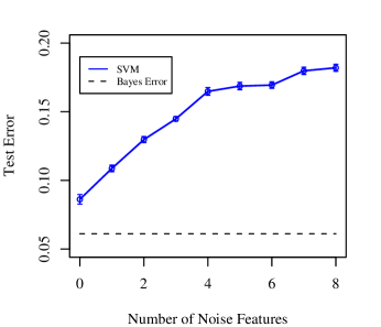
Figure 1: Mean test misclassification error when noise features are added to the skin of the orange simulation. Support vector machines with second order polynomial kernels are trained on data with 100 observations and tested on data with 1000 observations. Ten simulations are conducted for each new noise feature. The Bayes error is for this model is 0.0611.

We look at the support vector machine with non-linear kernels mathematically to gain an understanding of why irrelevant features have such an impact on the method. Given data $\operatorname{\mathbf{x}}_{i}\in\Re^{p}$ for $i=1\ldots n$ observations and $p$ features with the response $\operatorname{\mathbf{Y}}\in\{-1,1\}^{n}$. The kernel matrix, $\operatorname{\mathbf{K}}_{\operatorname{\mathbf{w}}}\in\Re^{n\times n}$ is defined by $\operatorname{\mathbf{K}}_{\operatorname{\mathbf{w}}}(i,i^{\prime})=k_{\operatorname{\mathbf{w}}}(\operatorname{\mathbf{x}}_{i},\operatorname{\mathbf{x}}_{i^{\prime}})=\left(\sum_{j=1}^{p}x_{ij}x_{i^{\prime}j}+1\right)^{d}$, for example with polynomial kernels. Recall that the support vector machine can be written as an unconstrained minimization problem with the hinge loss (Wahba et al., 1999).

$$\operatorname*{\mathrm{minimize}}_{\alpha,\alpha_{0}}\hskip 11.38109pt\sum_{i=1}^{n}\left[1-y_{i}\alpha_{0}-y_{i}(\operatorname{\mathbf{K}}\alpha)_{i}\right]_{+}+\lambda\alpha^{T}\operatorname{\mathbf{K}}\alpha.$$

Here, the coefficients $\alpha$ determine the support vectors which are sparse in the observations. Each feature, however, has the same impact on the objective since they are all given equal weight in the kernel matrix, thus explaining the poor performance with noise features. We, therefore, propose to place feature weights within the kernels to differentiate between true and noise features.

2.2 Feature Weighted Kernels

Before introducing feature weighted kernels, we give the data format. The data, as previously mentioned, $\operatorname{\mathbf{x}}_{i}\in\Re^{p}$ for $i=1\ldots n$ observations and can be written as the data matrix $\operatorname{\mathbf{X}}\in\Re^{n\times p}$. We assume that $\operatorname{\mathbf{x}}_{i}$ is standardized so that it has mean zero and variance one. For regression, the response $\operatorname{\mathbf{Y}}\in\Re^{n}$ and for classification, $\operatorname{\mathbf{Y}}\in\{-1,1\}^{n}$. In the previous example, we gave an example of a typical kernel, the polynomial kernel. In this section, we present feature weighted kernels, giving example for many common kernel types below. These kernels simply place a weight $\operatorname{\mathbf{w}}\in\Re^{p+}$ on each feature in the kernel.

• Inner Product Kernel:     $k_{\operatorname{\mathbf{w}}}(\operatorname{\mathbf{x}},\operatorname{\mathbf{x}}^{\prime})=\displaystyle\sum_{j=1}^{p}w_{j}x_{j}x^{\prime}_{j}$

• Gaussian (Radial) Kernel:     $k_{\operatorname{\mathbf{w}}}(\operatorname{\mathbf{x}},\operatorname{\mathbf{x}}^{\prime})=\mathrm{exp}\left(-\gamma\displaystyle\sum_{j=1}^{p}w_{j}(x_{j}-x^{\prime}_{j})^{2}\right)$

• Polynomial Kernels:     $k_{\operatorname{\mathbf{w}}}(\operatorname{\mathbf{x}},\operatorname{\mathbf{x}}^{\prime})=\left(\displaystyle\sum_{j=1}^{p}w_{j}x_{j}x^{\prime}_{j}\right)^{d},\hskip 11.38109ptk_{\operatorname{\mathbf{w}}}(\operatorname{\mathbf{x}},\operatorname{\mathbf{x}}^{\prime})=\left(\displaystyle\sum_{j=1}^{p}w_{j}x_{j}x^{\prime}_{j}+1\right)^{d}$

With these feature weighted kernels, we can define the kernel matrix and loss function for a kernel prediction method as $\operatorname{\mathbf{K}}_{\operatorname{\mathbf{w}}}\in\Re^{n\times n}$ such that $\operatorname{\mathbf{K}}_{\operatorname{\mathbf{w}}}(i,i^{\prime})=k_{\operatorname{\mathbf{w}}}(\operatorname{\mathbf{x}}_{i},\operatorname{\mathbf{x}}_{i^{\prime}})$.

2.3 KNIFE Optimization Problem

We incorporate these feature weighted kernels into the regression or classification model. The response, $\operatorname{\mathbf{Y}}$ is modeled by $\operatorname{\mathbf{Y}}=f(\operatorname{\mathbf{X}})$, where $f(\operatorname{\mathbf{x}}_{i})=\sum_{i^{\prime}=1}^{n}\alpha_{i}\operatorname{\mathbf{K}}_{w}(i,i^{\prime})$ for regression or $f(\operatorname{\mathbf{x}}_{i})=\mathrm{sign}(\alpha_{0}+\sum_{i^{\prime}=1}^{n}\alpha_{i}\operatorname{\mathbf{K}}_{w}(i,i^{\prime}))$ for classification, and $\alpha\in\Re^{n}$ are the coefficients that must be estimated. For a positive definite kernel, $\operatorname{\mathbf{K}}_{\operatorname{\mathbf{w}}}$, and $f(\operatorname{\mathbf{X}})$ a member of the reproducing kernel Hilbert space, $\mathcal{H}_{K_{\operatorname{\mathbf{w}}}}$, this problem can be written as a minimization problem of the form $\operatorname*{\mathrm{minimize}}_{f\in\mathcal{H}_{K_{\operatorname{\mathbf{w}}}}}\left[L(\operatorname{\mathbf{Y}},f(\operatorname{\mathbf{X}}))+\lambda||f||^{2}_{\mathcal{H}_{K_{\operatorname{\mathbf{w}}}}}\right]$, where $L(\operatorname{\mathbf{Y}},f(\operatorname{\mathbf{X}}))$ is the loss function. Some common examples of these include the hinge loss (support vector machine), squared error loss (regression) or binomial deviance loss (logistic regression).

To obtain a selection of important variables in a problem of this form, we need the weights to be both non-negative and sparse. To this end, we propose adding an $L_{1}$ penalty on the weights to induce sparsity and optimizing over the feasible set of non-negative weights that are less than one. This gives the KNIFE optimization problem as stated below.

$$\operatorname*{\mathrm{minimize}}_{\alpha,\operatorname{\mathbf{w}}}\hskip 14.22636pt f(\alpha,\operatorname{\mathbf{w}})=L(\operatorname{\mathbf{Y}},\operatorname{\mathbf{K}}_{\operatorname{\mathbf{w}}}\alpha)+\lambda_{1}\alpha^{T}\operatorname{\mathbf{K}}_{\operatorname{\mathbf{w}}}\alpha+\lambda_{2}\mathbf{1}^{T}\operatorname{\mathbf{w}}$$

subject to $$0\leq w_{j}<1,\textrm{ for all }j=1\ldots p.$$ (1)

The KNIFE optimization problem, (2.3), is non-convex and it is therefore extremely difficult to find a minimum, even for problems of small dimensions. To illustrate the non-convexities and understand our approach to finding a minimum, we offer an example. For SVMs with a Gaussian kernel, our optimization problem is given by the following.

$$\mathrm{minimize}\hskip 17.07164pt \sum_{i=1}^{n}\left[1-y_{i}\alpha_{0}-y_{i}\sum_{i^{\prime}=1}^{n}\alpha_{i^{\prime}}\mathrm{exp}\left(-\gamma\sum_{j=1}^{p}w_{j}(x_{ij}-x_{i^{\prime}j})^{2}\right)\right]_{+}$$

$$\qquad+\lambda_{1}\sum_{i=1}^{n}\sum_{i^{\prime}=1}^{n}\alpha_{i}\alpha_{i^{\prime}}\mathrm{exp}\left(-\gamma\sum_{j=1}^{p}w_{j}(x_{ij}-x_{i^{\prime}j})^{2}\right)+\lambda_{2}\mathbf{1}^{T}\operatorname{\mathbf{w}}$$

$$\mathrm{subject\hskip 2.84526ptto}\hskip 11.38109pt 0\leq w_{j}<1,\textrm{ for all }j=1\ldots p.$$ (2)

Here, notice that if we fix the weights, $\operatorname{\mathbf{w}}$, we simply have a convex optimization problem that is equivalent to solving the SVM problem. If we fix $\alpha$ and $\alpha_{0}$, however, the problem is not convex in $\operatorname{\mathbf{w}}$. This results from the fact that the coefficients $\alpha$ are both positive and negative. One could approach this as a difference of convex programming problem, a direction taken in (Argyriou et al., 2006) for a slightly different problem. This method of minimizing 2.3 is computationally prohibitive.

Thus, we propose an alternative algorithmic approach by using iterative convexifications of the weights within the kernel. This is discussed in the next section where we present the KNIFE algorithm.

3 KNIFE Algorithm

Given the KNIFE optimization problem based on the feature weighted kernels, we propose an algorithm to minimize the penalized loss function (2.3) for any kernel classification or regression method. The algorithm alternates between minimizing with respect to the coefficients $\alpha$ and the feature weights $\operatorname{\mathbf{w}}$. For non-linear kernels, we need to convexify the weights to obtain a feasible optimization problem. But, to understand the fundamentals of the algorithm we first discuss KNIFE for linear kernels in Section 3.1. We then present the algorithm for non-linear kernels, in Section 3.2, also discussing kernel convexification. Finally, we give connections to several other regression and non-parametric methods, Section 3.3 along with KNIFE solution properties and convergence results, Section 3.4.

3.1 Linear Kernels

We give the coordinate-wise KNIFE algorithm for linear kernels which form the foundation of the algorithm for non-linear kernels. With linear kernels, the kernel matrix becomes $\operatorname{\mathbf{K}}_{\operatorname{\mathbf{w}}}=\operatorname{\mathbf{X}}\operatorname{\mathbf{W}}\operatorname{\mathbf{X}}^{T}$ where $\operatorname{\mathbf{W}}=\mathrm{diag}(\operatorname{\mathbf{w}})$. This gives the following objective function.

$$f(\alpha,\operatorname{\mathbf{w}})=L(\operatorname{\mathbf{Y}},\operatorname{\mathbf{X}}\operatorname{\mathbf{W}}\operatorname{\mathbf{X}}^{T}\alpha)+\lambda_{1}\alpha^{T}\operatorname{\mathbf{X}}\operatorname{\mathbf{W}}\operatorname{\mathbf{X}}^{T}\alpha+\lambda_{2}\mathbf{1}^{T}\operatorname{\mathbf{w}}.$$

Letting $\beta=\operatorname{\mathbf{X}}^{T}\alpha$, we arrive at

$$f(\beta,\operatorname{\mathbf{w}})=L(\operatorname{\mathbf{Y}},\operatorname{\mathbf{X}}\operatorname{\mathbf{W}}\beta)+\lambda_{1}\beta^{T}\operatorname{\mathbf{W}}\beta+\lambda_{2}\mathbf{1}^{T}\operatorname{\mathbf{w}}.$$ (3)

Here, notice that $f(\beta,\operatorname{\mathbf{w}})$ is a bi-convex function of $\beta$ and $\operatorname{\mathbf{w}}$, meaning that if we fix $\beta$, $f(\cdot,\operatorname{\mathbf{w}})$ is convex in $\operatorname{\mathbf{w}}$ and if we fix $\operatorname{\mathbf{w}}$, $f(\beta,\cdot)$ is convex in $\beta$.

This biconvex property leads to a simple coordinate-wise algorithm for minimization, minimizing first with respect to $\beta$ with $\operatorname{\mathbf{w}}$ fixed and then with respect to $\operatorname{\mathbf{w}}$. While this coordinate descent algorithm is monotonic, meaning that each iteration decreases the objective function $f(\beta,\operatorname{\mathbf{w}})$, it does not necessarily converge to the global minimum. If the objective function satisfies certain smoothness conditions (discussed in Section 3.4), then coordinate descent converges to a stationary point (Tseng, 2001).

For linear kernels, the optimization problem is still non-convex but satisfies certain convex properties, namely bi-convexity in the weights and the coefficients. This is the approach that we will take for non-linear kernels, namely linearizing the kernels with respect to the weights to obtain a surrogate function which is convex in $\operatorname{\mathbf{w}}$ as presented in the following section.

3.2 KNIFE Algorithm

We linearize kernels with respect to the feature weights to obtain a function convex in the weights and hence conducive to easy minimization. From the previous section, we saw that if the function is linear in the feature weights, then we can apply a block coordinate-wise algorithm, finding the coefficients and then finding the weights. Thus for non-linear kernels, we need to linearize kernels in such a way that leads to an algorithm minimizing the objective function (2.3).

The linearized kernels are given by $\tilde{k}_{\operatorname{\mathbf{w}}}$ as defined below.

$$\tilde{k}_{\operatorname{\mathbf{w}}^{(t)}}(i,i^{\prime})=k_{\operatorname{\mathbf{w}}^{(t-1)}}(i,i^{\prime})+\bigtriangledown k_{\operatorname{\mathbf{w}}^{(t-1)}}(i,i^{\prime})^{T}(\operatorname{\mathbf{w}}^{(t)}-\operatorname{\mathbf{w}}^{(t-1)}).$$ (4)

Notice that $\tilde{k}_{\operatorname{\mathbf{w}}}(i,i^{\prime})$ is the linearization of the $(i,i^{\prime})^{th}$ element of the kernel matrix $\operatorname{\mathbf{K}}_{\operatorname{\mathbf{w}}}$. Here, $\operatorname{\mathbf{w}}^{(t-1)}$ is the weight vector from the previous iteration. Minimization is done with respect to $\operatorname{\mathbf{w}}^{(t)}$.

Linearizing the kernels in this manner, however, is not ideal for two reasons. First, notice that in non-linear kernels, the weights are placed on the cross products or squared distance of the data vectors within a non-linear function. Thus, we need to place the weights on the same scale as the data. (Note that reparameterizing the linear kernels in terms of $\beta$ solves this problem for linear kernels.) Secondly, this naive linearization is not conducive to developing a stable minimization algorithm. To achieve these objectives, we linearize kernels with respect to $\operatorname{\mathbf{w}}^{2}$ instead of $\operatorname{\mathbf{w}}$. The differences between these can be clearly seen with an example of the gradient of a polynomial kernel with squared feature weights,

$$\bigtriangledown k_{\operatorname{\mathbf{w}}^{(t-1)}}(i,i^{\prime})_{k}=2dw^{(t-1)}_{k}x_{ik}x_{i^{\prime}k}\left(\sum_{j=1}^{p}w^{2^{(t-1)}}_{j}x_{ij}x_{i^{\prime}j}+1\right)^{d-1}.$$

Here, notice that the gradient is scaled by the weights of the previous iteration, $\operatorname{\mathbf{w}}^{(t-1)}$. Thus, if several weights were previously set to zero, the gradient in those directions is zero meaning that the weights will remain zero in all subsequent iterations of the algorithm. This feature, first of all maintains sparsity in the feature weights throughout the algorithm, and secondly limits the number of directions in which the weight vector can move in succeeding iterations. The second attribute can be critical to algorithm convergence (see Section 3.4).

Thus, for non-linear kernels, our KNIFE objective changes slightly to allow for linearization of the kernels with squared feature weights.

$$f(\alpha,\operatorname{\mathbf{w}})=L(\operatorname{\mathbf{Y}},\operatorname{\mathbf{K}}_{\operatorname{\mathbf{w}}^{2}}\alpha)+\lambda_{1}\alpha^{T}\operatorname{\mathbf{K}}_{\operatorname{\mathbf{w}}^{2}}\alpha+\lambda_{2}\mathbf{1}^{T}\operatorname{\mathbf{w}}.$$ (5)

We present the KNIFE algorithm for non-linear kernels in Algorithm 1.

Algorithm 1 KNIFE Algorithm

1. Initialize $\alpha^{(0)}$ and $\operatorname{\mathbf{w}}^{(0)}$ where $0<w^{(0)}_{j}<1$ for $j=1\ldots p$.

2. Minimize $f(\alpha^{(t-1)},\operatorname{\mathbf{w}}^{(t-1)})$ with respect to $\alpha^{(t-1)}$.

3. Linearize $\operatorname{\mathbf{K}}_{\operatorname{\mathbf{w}}^{2}}$ element-wise giving $f(\alpha^{(t)},\tilde{\operatorname{\mathbf{w}}}^{(t-1)})$.

4. Minimize $f(\alpha^{(t)},\tilde{\operatorname{\mathbf{w}}}^{(t-1)})$ with respect to $\tilde{\operatorname{\mathbf{w}}}^{(t-1)}$ subject to $0\leq w_{j}<1$ for $j=1\ldots p$.

5. Repeat steps 2-4 until convergence.

We will take a closer look at the KNIFE algorithm by presenting an example with support vector machines. Step 2 is an SVM problem finding the coefficients.

$$\mathrm{minimize}\hskip 5.69054pt\sum_{i=1}^{n}\left[1-y_{i}\alpha_{0}-y_{i}(\operatorname{\mathbf{K}}_{\operatorname{\mathbf{w}}^{2}}\alpha)_{i}\right]_{+}+\lambda_{1}\alpha^{T}\operatorname{\mathbf{K}}_{\operatorname{\mathbf{w}}^{2}}\alpha.$$

Now, we define

$$\operatorname{\mathbf{B}}\in\Re^{n\times n}:\hskip 5.69054pt \operatorname{\mathbf{B}}_{ii^{\prime}}=k_{\operatorname{\mathbf{w}}^{2^{(t-1)}}}(i,i^{\prime})-\bigtriangledown k_{\operatorname{\mathbf{w}}^{2^{(t-1)}}}(i,i^{\prime})^{T}\operatorname{\mathbf{w}}^{(t-1)}$$

$$\operatorname{\mathbf{A}}\in\Re^{n\times p}:\hskip 5.69054pt \operatorname{\mathbf{A}}_{ii^{\prime}}=\sum_{i^{\prime}=1}^{n}\alpha_{i^{\prime}}\bigtriangledown k_{\operatorname{\mathbf{w}}^{2^{(t-1)}}}(i,i^{\prime})^{T}.$$

Then, the objective function in Step 4 becomes

$$\textrm{minimize }\sum_{i=1}^{n}\left[1-y_{i}\alpha_{0}-y_{i}(\operatorname{\mathbf{B}}\alpha)_{i}-y_{i}(\operatorname{\mathbf{A}}\operatorname{\mathbf{w}})_{i}\right]_{+}+\lambda_{1}\alpha^{T}\operatorname{\mathbf{A}}\operatorname{\mathbf{w}}+\lambda_{2}\mathbf{1}^{T}\operatorname{\mathbf{w}}.$$

Notice that Step 4 reduces to a loss function that is linear in $\operatorname{\mathbf{w}}$. In fact, for any loss function, the objective function of Step 4 becomes $L(\operatorname{\mathbf{Y}},\operatorname{\mathbf{B}}\alpha+\operatorname{\mathbf{A}}\operatorname{\mathbf{w}})$.

Thus, the KNIFE algorithm iterates between finding the coefficients of the regression or classification problem and then finding the sparse set of feature weights. With linearizations of the kernels with respect to the squares of the weights, the iterative optimization to find coefficients and weights are both problems of the same form but in different spaces. For example, with squared error loss, minimization with respect to the coefficients is a form of least squares problem in $n$ dimensional space whereas minimization with respect to the weights in the linearized kernel is also a form of least squares problem in $p$ dimensional feature space. Now that we have presented the algorithm framework, we go back to the skin of the orange example to briefly demonstrate the KNIFE algorithm in action.

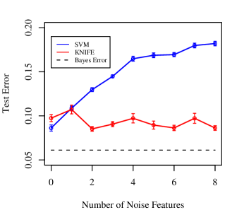
Figure 2: Mean test misclassification error when noise features are added to the skin of the orange simulation. SVMs and KNIFE for SVMs with second order polynomial kernels are trained on data with 100 observations and tested on data with 1000 observations. Ten simulations are conducted for each new noise feature. The Bayes error is for this model is 0.0611.

In Figure 2, we present the misclassification error for the KNIFE as well as the SVM. Here, we see that KNIFE preforms well even when many noise features are added to the model. To understand the reason for this performance improvement and further examine the KNIFE problem and algorithm, we discuss several connections to existing methods and present convergence results.

3.3 Connections with Other Methods

While the optimization problem (2.3) may appear unfamiliar, there are several variations that are the same or similar in form to many existing methods. We first begin by looking at linear kernels for regression problems with squared error loss. A form of the objective with linear kernels is given in the previous section, (3). We give this and an equivalent form for comparison purposes.

$$\mathrm{minimize}\hskip 14.22636pt ||\operatorname{\mathbf{Y}}-\operatorname{\mathbf{X}}\operatorname{\mathbf{W}}\beta||_{2}^{2}+\lambda_{1}\beta^{T}\operatorname{\mathbf{W}}\beta+\lambda_{2}||\operatorname{\mathbf{w}}||_{1}$$ (6)

or $$||\operatorname{\mathbf{Y}}-\operatorname{\mathbf{X}}\tilde{\beta}||_{2}^{2}+\lambda_{1}\tilde{\beta}^{T}\operatorname{\mathbf{W}}^{-1}\tilde{\beta}+\lambda_{2}||\operatorname{\mathbf{w}}||_{1}$$ (7)

subject to $$\operatorname{\mathbf{w}}\geq 0.$$

These are closely related to several common regression methods. First, if we let $\lambda_{2}=0$ and $\operatorname{\mathbf{w}}=\mathbf{1}$ in (6), we get ridge regression. If we let $\lambda_{1}=0$, then we have the form of the non-negative garrote (Breiman, 1995). The form of both (6) and (7) is very similar to the elastic net which places an $L_{1}$ and $L_{2}$ penalty on the coefficients (Zou and Hastie, 2005). In the KNIFE, however, the $L_{1}$ penalty is not on the coefficients, but on the weights that multiply the coefficients. Letting $\lambda_{1}=0$, we get a problem very similar in structure and intent to the lasso. Also, if we let $\lambda_{2}=0$, then we have a problem that puts weights on the $L_{2}$ penalty on the coefficients. This is similar to the adaptive lasso which places weights on the $L_{1}$ penalty on the coefficients (Zou, 2006).

In addition to these methods, a special case of the COSSO (Component Selection and Smoothing Operator) which estimates non-parametric functions give (6) and (7) exactly (Lin and Zhang, 2007). This method in theory minimizes the sums of squares between the response and a function with an $L_{2}$ penalty on the projection of the function scaled by the inverse of a non-negative weight. This proposed theoretical form is also the form of (7). In addition, the COSSO employs an algorithm which first fits a smoothing spline and then fits a non-negative garrote, noting that these steps can be repeated. This algorithmic approach is also analogous to the KNIFE algorithm for the special case of squared error loss with linear kernels.

These similarities between other regression methods and KNIFE hold with other forms of loss functions also. For support vector machines, we have a problem similar to the $L_{1}$ and $L_{2}$ support vector machines in the same way that the inner-product squared error loss KNIFE relates to ridge and lasso regression. The same is true of $L_{1}$ and $L_{2}$ regularized logistic regression.

3.4 Convergence of KNIFE

In this section we discuss the convergence of the KNIFE algorithm and the properties of the KNIFE solution, also giving numerical examples. As previously discussed, the KNIFE objective is highly non-convex and thus it is difficult to assert any claims on the convergence of the KNIFE algorithm or the optimality of the KNIFE solution. For special cases, however, we can guarantee convergence of the KNIFE algorithm to a stationary point.

Claim 1

If the KNIFE algorithm finds a unique minimum for the coefficients, $\alpha$, and the weights, $\operatorname{\mathbf{w}}$, in each step and the loss function and kernel are continuously differentiable, then the KNIFE algorithm monotonically decreases the objective and converges to a stationary point of $f(\alpha,\operatorname{\mathbf{w}})$.

Proof  Differentiability of the loss function and kernel implies that $f(\alpha,\operatorname{\mathbf{w}})$ is regular on its domain. This along with unique minima in both blocks of coordinates satisfies conditions for monotonic convergence to a stationary point for non-convex functions. In theory, differentiability can be relaxed to weaker conditions for regularity (Tseng, 2001).  

The conditions in Claim 1 are satisfied with strictly convex, differentiable loss functions with linear kernels. An example here is the squared error loss and linear kernel given in (6). We have noted that these examples are bi-convex, and thus the KNIFE algorithm simply iterates between minimization with respect to the coefficients and then the feature weights. Hence, for these special cases of KNIFE, we are guaranteed to converge to a stationary point. We must note, however, that for non-convex functions, there can be potentially many stationary points. Thus, the stationary point at which KNIFE arrives will depend on the random starting values of the weights. For this reason, we recommend initializing the KNIFE algorithm at several random starting points and taking the solution which gives the minimum objective value.

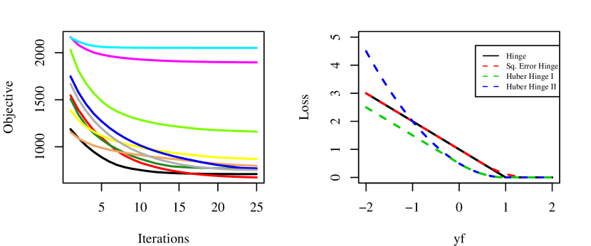
Figure 3: (a) KNIFE objective for iterations of the KNIFE algorithm starting at 10 random set of weights. Here, a radial kernel with squared error loss is used. (b) Smooth approximations to the non-differentiable hinge loss for the support vector machine.

We pause to note the importance of loss function differentiability. While many loss functions, such as squared error and binomial deviance, are continuously differentiable, there is one notable exception, namely the hinge loss of support vector machines. Because of the necessity of smoothness conditions for non-convex functions as proven in Tseng (2001), the coordinate-wise minimizations of KNIFE for SVMs may never converge. Hence, we suggest using surrogate loss functions to approximate the hinge loss. Several smooth versions of this loss have been suggested, including squared error hinge and a Huberized hinge loss (Wang et al., 2008), as shown in Figure 3 (b). These both have been shown to approximate the results of the support vector machine well. Thus, we propose that instead of using the KNIFE algorithm directly with SVMs, to run the algorithm with a smoothed version of the hinge loss. Then, given the set of optimal weights, calculate the SVM coefficients using the hinge loss. Our experience reveals that in general, this scheme finds a reasonable solution which decreases the original objective function with hinge loss.

While we have discussed KNIFE for linear kernels, we have not given any results on the convergence of KNIFE for non-linear kernels in which we do not find the unique minimum with respect to the feature weights in each step. As previously discussed, for non-linear kernels, the objective is highly non-convex with respect to the feature weights. Thus, we cannot claim any theoretical convergence results for KNIFE with respect to these kernels. In numerical examples, however, for differentiable, convex loss functions and kernels, the KNIFE algorithm converges and decreases the objective monotonically. This is shown in an example with radial kernels and squared error loss in Figure 3 (a).

There are several intuitive reasons explaining observed convergence of KNIFE for convex, differentiable losses and kernels. First, if the kernel is convex and differentiable, then the linearization with respect to the square of the weights is a global under-estimator of the kernel. Thus, one can surmise that minimizing the KNIFE objective with the linearized kernel will tend to decrease the objective, except for pathological cases. If we restrict the feature weights in each iteration to be close to previous weights, we know that a linear approximation is close to the true function if the function is continuous. For this reason, linearizing the kernel with the squared weights is crucial since it restricts the search directions for the weight vector, keeping the weights close to the previous set of weights. Also, since the minimization with respect to the feature weights is followed by estimating the coefficients, for which the objective is convex, the KNIFE algorithm will, in general, decrease the KNIFE objective. Since the objective is bounded below, this explains the observed convergence of the KNIFE algorithm in numerical examples. We surmise that with possibly stricter conditions on the objective function, stronger theoretical convergence results may be attainable even for non-linear kernels. Overall, while we do not give precise convergence results, we recommend using KNIFE with convex, differentiable losses and kernels.

3.5 KNIFE Feature Path Algorithm

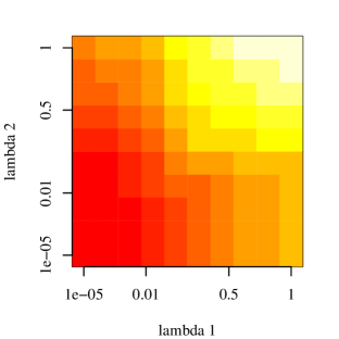
Figure 4: Values of the KNIFE objective for several penalty parameter, $\lambda_{1}$ and $\lambda_{2}$ values. Darker blocks represent smaller values of the objective.

Since the KNIFE method uses regularization to extract important features, we can modify KNIFE to give a path-wise algorithm resulting in non-linear feature paths. Regularization paths are common in linear regression problems where the values of the coefficients are given for each value of a penalty parameter used. Our path algorithm is similar. For KNIFE, however, we have two penalty parameters, $\lambda_{1}$ and $\lambda_{2}$. Both of these parameters place a penalty on the feature weights and thus are related. We explore this relationship in Figure 4 where we give values of the KNIFE objective (2.3) for various penalty parameter values.

While both parameter values effect the feature weights and the value of the objective, we have pointed out that the parameter $\lambda_{2}$ encourages sparsity. Hence, when formulating a feature path algorithm, we focus on $\lambda_{2}$, fixing the value of $\lambda_{1}$. In general, setting $\lambda_{1}=1$ (or if the loss function is given as $\frac{1}{n}L(\operatorname{\mathbf{Y}},f(\operatorname{\mathbf{X}}))$, then $\lambda_{1}=\frac{1}{n}$) performs reasonably well and is thus our default value for the remainder of the paper. Now, setting $\lambda_{2}=0$ gives no direct penalty on the feature weights and thus all features are permitted to be non-zero. Hence, the path algorithm varies from $\lambda_{2}=0$ where all feature weights are non-zero to $\lambda_{2}=M$, where $M$ is the value at which all weights become zero. The path-wise algorithm is given below in Algorithm 2.

Algorithm 2 KNIFE Feature Path Algorithm

1. Fix $\lambda_{1}$, set $\lambda_{2}=0$ and initialize $\alpha$ and $\operatorname{\mathbf{w}}$.

2. Fit KNIFE with $\alpha^{(t-1)}$ and $\operatorname{\mathbf{w}}^{(t-1)}$ as warm starts.

3. Increase $\lambda_{2}$.

4. Repeat Steps 2-3 until $\operatorname{\mathbf{w}}=\mathbf{0}$.

Algorithm 2 maps out feature paths because of two attributes of the original KNIFE algorithm. First, recall that in KNIFE we linearize kernels with respect to the square of the weights, creating an algorithm that is sticky at zero. This means that as we increase $\lambda_{2}$ once a particular feature’s weight is set to zero, it cannot ever become non-zero. This attribute permits us to efficiently use warm starts for the coefficients and weights, speeding computational time considerably. Also, with warm starts and a small increase in $\lambda_{2}$, one can use a single update of the coefficients and weights at each iteration to approximate the feature paths.

We pause briefly to compare this path algorithm to the well known coefficient paths of the lasso and LAR (Least Angle Regression) algorithms (Efron et al., 2004). In both of these regularization paths, the algorithm begins with no variables in the model and incrementally includes coefficients who most correlate with the response. In our KNIFE path algorithm, however, we begin with all features in the model and incrementally eliminate the features that are uncorrelated (in the kernel space) with the response. Thus, the KNIFE path algorithm can be thought of as a regularization approach to backwards elimination for kernels. Also, the lasso regularization paths permit coefficient paths to cross zero and enter and re-enter the model. KNIFE does not allow this because of the sticky property of the feature weights, meaning that one a feature weight is set to zero it cannot move away from zero. The KNIFE path algorithm is then like a kernel analog of other common coefficient regularization paths.

4 Results

In this section, we explore the performance of the KNIFE algorithm and the KNIFE path algorithm on both real and simulated data. We demonstrate KNIFE in conjunction with two predictions methods, least squares and support vector machines. Three of the most common kernels, the inner product kernel, polynomial kernels, and Gaussian (radial) kernels are used. For three simulations, we give results both in terms of prediction error and feature path realizations, comparing KNIFE to existing feature selection methods such as Sure Independence Screening (SIS) (Fan and Lv, 2008) and Recursive Feature Elimination (RFE) (Guyon et al., 2002). Finally, we give results on gene selection in colon cancer microarray data (Alon et al., 1999) and feature selection in vowel recognition data (Hastie et al., 2001) and Parkinson’s disease data (Little et al., To Appear).

4.1 Simulations

We present three simulation examples to demonstrate the performance of KNIFE: linear regression, non-linear regression, and non-linear classification. Each of the three simulations were repeated fifty times and error rates are averaged. Training sets were generated of dimension $100\times 10$ and test sets were of dimension $1000\times 10$. Parameters for KNIFE and all other comparison methods were found by taking the parameter giving the minimum error on a separate validation set of dimension $1000\times 10$. For all KNIFE methods, $\lambda_{1}$ was fixed at 1 and $\lambda_{2}$ was found by validation. To be fair, we validate one parameter for each comparison method also. All simulations include true features are noise features as specified below.

4.1.1 Linear Regression

We simulate data from a linear model to compare the KNIFE method using an inner product kernel with squared error loss to common regression methods. Recall that this most basic form of KNIFE given in (6) is closely related to many regression methods as discussed in Section 3.3. This simulation is then given more to illustrate these connections between regression methods than to promote the use of KNIFE for linear regression.

In this simulation, we have ten features, five of which are random noise. The true coefficients are then $\beta^{true}=[6,-4,3,2,-2,0,0,0,0,0]^{T}$. We take the data, $\operatorname{\mathbf{x}}\in\Re^{p}$, to be standard normal and the response is given by the following model. $y=\operatorname{\mathbf{x}}\beta^{true}+\epsilon$, where $\epsilon\sim N(0,1)$. The results in terms of training and test error are given in Table 1.

Method	Training Error	Test Error
Least Squares	0.9220 (.0026)	1.0937 (.0015)
Ridge	0.9220 (.0026)	1.0937 (.0015)
Lasso	0.9452 (.0026)	1.0725 (.0014)
Elastic Net	0.9472 (.0026)	1.0746 (.0014)
KNIFE	0.9377 (.0026)	1.0738 (.0016)

Table 1: Simulation results for linear regression. The data has ten features, five of which are noise features. Mean squared error on training and test sets are given with the standard error in parenthesis. The two best performing methods are in bold.

These results show that the linear KNIFE method performs similarly to other sparse regression methods such as the lasso and elastic net.

4.1.2 Non-linear Regression

To investigate KNIFE with other kernels, we simulate a sinusoidal, non-linear regression problem. Here we still use squared error loss but use KNIFE with radial and second order polynomial kernels. We compare KNIFE to linear ridge regression and kernel or generalized ridge regression. In addition we give results for the filtering method SIS and the selection method RFE both used with kernel ridge regression. We note here that the scale parameter, $\gamma$, for the radial kernel is set to $\gamma=1/p$, a commonly used default for the non-KNIFE methods using radial kernels. This simulation, like the first, also has ten features with five of them random noise. The true coefficients and data are the same as in the previous simulation, but we change the model to be $y=\mathrm{sin}(\operatorname{\mathbf{x}})\beta^{true}+\epsilon$, thus adding a non-linear element.

Method	Training Error	Test Error
Ridge	4.8337 (.0202)	6.2589 (.0109)
Kernel Ridge	0.0874 (.0005)	6.1239 (.0106)
SIS/ Kernel Ridge	0.9592 (.0122)	3.8119 (.0389)
RFE/ Kernel Ridge	0.7848 (.0074)	5.4386 (.0366)
KNIFE/ Kernel Ridge (radial)	2.1187 (.0058)	3.5498 (.0083)
KNIFE/ Kernel Ridge (polynomial)	5.2376 (.0181)	6.8591 (.0186)

Table 2: Simulation results for sinusoidal, non-linear regression. The data has ten features, five of which are noise features. Mean squared error on training and test sets are given with the standard error in parenthesis. The two best performing methods are in bold.

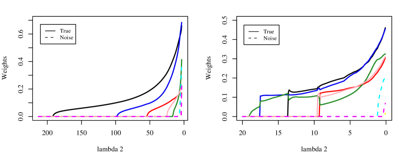
Figure 5: Feature path realizations of KNIFE for polynomial kernels of order 2 (left) and radial kernels (right) with a squared error loss function. Data of dimension $100\times 10$ was simulated from the sinusoidal simulation with five true features and five noise features. KNIFE for both kernel types gives non-zero weights to the five true features for much of the feature paths.

In Table 2, we report the mean squared error for the training and test sets over the fifty simulations. We see that KNIFE with radial kernels outperforms competing methods including the commonly used SIS and RFE methods for extracting important features. In addition, the feature weights of KNIFE are very stable, with only five total noise features given a non-zero weight for radial kernels out of the all five noise features in fifty simulations. Among the KNIFE methods, a radial kernel gives much better error rates than the second order polynomial, indicating that choosing the wrong kernel can be problematic. To investigate this further we give the entire feature path realizations for both radial and polynomial kernels in Figure 5. We see that while the polynomial kernel gives much smoother feature paths, the radial kernel estimates the true features for a much larger portion of the feature path.

Here we make a brief note about the feature weights in radial kernels. In general, the scaling factor $\gamma$ can be extremely important in radial kernels, but for KNIFE, we do not need to include any scale factors. The feature weights themselves act as automatic scaling factors, adjusting to fit the data. This is seen in the radial feature paths of Figure 5 where all of the feature weights adjust when one new non-zero feature is added to the model.

4.1.3 Non-linear Classification

We use support vector machines to assess KNIFE’s performance on non-linear classification simulations. The simulation is the skin of the orange simulation, previously presented as a motivating example, with four true features and six noise features (Hastie et al., 2001). Here, the first class has four standard normal features, $\operatorname{\mathbf{x}}_{1},\operatorname{\mathbf{x}}_{2},\operatorname{\mathbf{x}}_{3},\operatorname{\mathbf{x}}_{4}$, and the second class has the same conditioned on $9\leq\sum_{j=1}^{4}\operatorname{\mathbf{x}}_{j}^{2}\leq 16$. Thus, the model has one class which is spherical with the second class surrounding the sphere like the skin of the orange.

Method	Training Error	Test Error
SVM	0 (0)	0.1918 (.0006)
SIS / SVM	0 (0)	0.3689 (.0016)
RFE / SVM	0.0206 (.0007)	0.1937 (.0014)
KNIFE	0.0468 (.0006)	0.1136 (.0009)

Table 3: Average misclassification errors for the skin of the orange simulation with four true features and six noise features. All methods use support vector machines with second order polynomials. Standard errors are in parenthesis with the two best performing methods in bold.

The results of this simulation in terms of misclassification error on he training and test sets are presented in Table 3. A second order polynomial kernel was used for all methods. We note that KNIFE was used with the squared error hinge loss approximation to the hinge loss of the SVM. On this simulation also, KNIFE outperforms both regular SVMs and other common feature selection methods. A portion of the feature paths are presented in Figure 6. Here, two out of the four true features are selected for much of the path. This is due to the fact that all four true features are of the same distribution for this simulation. Here, we also comment on a unique property of KNIFE for support vector machines. The SVM is sparse in the observation space, meaning that only a subset of the observations are chosen as support vectors. With KNIFE SVM, we get sparsity in the feature space also, leaving us with an important sub-matrix of observations and features that can limit computational storage for prediction purposes.

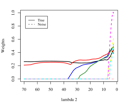
Figure 6: Feature path realization of KNIFE for polynomial kernels of order 2 for support vector machines (hinge loss). Data of dimension $100\times 10$ was simulated from the skin of the orange simulation with four true features and six noise features.

4.2 Example Data

Finally, we apply KNIFE to three feature selection applications, beginning with microarray data. With thirty thousand human genes, doctors often need a small subset of genes to test that are predictive of a disease. For this application, we use microarray data on colon cancer given in Alon et al. (1999). The dataset consists of 62 samples, 22 of which are normal and 40 of which are from colon cancer tissues. The genes are already pre-filtered, consisting of the 2,000 genes with the highest variance across samples.

# Genes	SIS/SVM	RFE/SVM	KNIFE/SVM
2000	0.0355 (.0062)	0.0355 (.0062)	0.0387 (.0062)
500	0.0419 (.0027)	0.1290 (.0050)	0.0484 (.0059)
250	0.0516 (.0027)	0.1452 (.0063)	0.0516 (.0057)
100	0.0613 (.0039)	0.1677 (.0066)	0.0710 (.0054)
50	0.0645 (.0043)	0.1774 (.0065)	0.0806 (.0057)
25	0.0677 (.0024)	0.1742 (.0041)	0.0871 (.0055)
15	0.0742 (.0040)	0.1484 (.0049)	0.1065 (.0059)
10	0.0968 (.0046)	0.1581 (.0060)	0.1194 (.0061)

Table 4: Average misclassification rates with standard errors on ten randomly created test sets for the colon cancer microarray data. All methods use a linear support vector machine.

For this analysis, we use a linear SVM for classification, comparing KNIFE to gene filtering using SIS and RFE. We evaluate eight subsets of previously fixed numbers of genes on the three methods. For the gene selection with RFE, we begin by eliminating 50 genes, ten genes and then one gene at each step as outlined in Guyon et al. (2002). To determine predictive ability, we split the samples randomly into training and test sets of equal sizes. This is repeated ten times and misclassification rates are averaged. These results are given in Table 4.

# Genes	SIS/SVM	KNIFE/SVM
2000	0.5913	0.5913
500	0.6365	0.5969
250	0.6451	0.5981
100	0.6534	0.5951
50	0.6674	0.5964
25	0.6652	0.5898
15	0.6910	0.5946
10	0.7139	0.5895

Table 5: Median of absolute pair-wise correlations of genes selected by each method on the colon cancer microarray data.

The results indicate that KNIFE outperforms the commonly used RFE filtering method for all subsets of genes. For smaller subsets, however, SIS filtering performs the best in terms of test error. While the subset of genes determined by SIS may be good in terms of prediction, often researchers are interested in a subset of genes that are members of different pathways and are hence less correlated. For each of the subsets, we report the median of the absolute pair-wise correlations of the genes selected by both SIS and KNIFE in Table 5. Here, we notice that KNIFE selects a group of genes that have around that same median correlation as the original 2,000 genes. On the other hand, SIS filtering tends to select highly correlated groups of genes that might not be as desirable for research purposes.

The vowel recognition dataset Hastie et al. (2001) consists of eleven classes of vowels broken down into ten features which fifteen individuals were recorded saying six times. For illustration, we apply a radial kernel SVM and KNIFE to classify between vowels ’i’ and ’I’ based on ten features shown on the left in Figure 7. We use five fold cross-validation to determine the margin size for the SVM and the $\lambda_{2}$ value for KNIFE. Both methods were trained on a dataset with 48 instances of each vowel and tested with 42 instances of each. KNIFE gives a test misclassification error of 8.3% while the SVM gives an error of 19.1%. We see, in Figure 7 that KNIFE selects six features that are indicative of the two vowel types. For some other pairs of vowels, however, KNIFE does not perform better than SVMs indicating that all ten features may be needed for classification of other vowels.

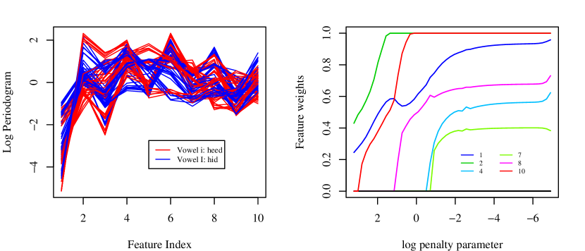
Figure 7: Vowel recognition data for vowels ’i’ and ’I’ (left) with KNIFE feature paths for classifying the two vowels using a support vector machine with radial kernels (right). Five fold cross-validation on the training set chose to include the six features shown. KNIFE gives a test misclassification error of 8.3%, while a radial kernel SVM has 19.1% test error.

The Parkinson’s disease dataset consists of 22 biomedical voice measurements from 31 individuals, 23 of which have Parkinson’s disease (Little et al., To Appear). Five-fold cross-validation by individuals was used to choose the optimal margin for SVMs and $\lambda_{2}$ for KNIFE. We then randomly divided the data (by individuals) into training and test sets of equal size. Both KNIFE and the SVM were able to perfectly separate diseased from healthy individuals in all 100 trials. KNIFE, however, chooses an average of eight features for use in the classification. In Table 6, we give the top eleven most frequently selected features and compare these to the features selected by the model in Little et al. (To Appear), which were selected by filtering and assessing all possible feature combinations. Several of the features measure similar attributes and thus are not often selected together. Three features, however, were selected in all 100 models and given a large weight.

Feature	Explanation	Average	Times	Selected by
		Weight	Selected	Little et al.
DFA	Signal fractal scaling exponent	0.902	100/100	Yes
MDVP:Fo(Hz)	Average fundamental frequency	0.879	100/100	No
RPDE	Dynamical complexity measure	0.803	100/100	Yes
HNR	Ratio to noise of tonal components	0.669	87/100	Yes
spread 2	Fundamental frequency variation	0.668	83/100	No
spread 1	Fundamental frequency variation	0.388	72/100	No
D2	Dynamical complexity measure	0.168	68/100	Yes
MDVP:Flo(Hz)	Minimum fundamental frequency	0.133	58/100	No
MDVP:RAP	Fundamental frequency variation	0.229	33/100	No
PPE	Fundamental frequency variation	0.294	32/100	Yes
Shimmer:APQ3	Variation in amplitude	0.106	16/100	No

Table 6: Features, or biomedical voice measurements, selected by KNIFE with radial kernel SVMs for classification of healthy individuals from those with Parkinson’s disease. The average weight and the number of times out of 100 which KNIFE selects the feature are given. We also report whether the feature was selected by Little et al. (To Appear) for use in their radial SVM classifier.

5 Discussion

We have presented a method for selecting important features with non-linear kernel regression and classification methods: KerNel Iterative Feature Extraction (KNIFE). The KNIFE optimization problem forms feature weighted kernels and seeks to find the minimum of a penalized, feature weighted kernel loss function with respect to both the coefficients and the feature weights. We have given the KNIFE algorithm which iteratively finds the coefficients, linearizes the kernels, then finds the set of feature weights. This algorithm, under broad conditions, converges and decreases the KNIFE objective for each iteration. A path-wise algorithm is also given for the kernel feature weights. Finally, we have demonstrated the utility of KNIFE for feature selection and kernel prediction for several example simulations and microarray data.

Computationally, the KNIFE algorithm compares favorably to existing kernel feature selection methods, which the exception of simple feature filtering methods including SIS. The KNIFE algorithm iterates between an optimization problem in the $n$-dimensional feature space and then a $p$-dimensional feature space. For comparison, RFE solves a problem in $n$-dimensional space several times, checking each remaining feature at each iteration. Thus, several kernels must be computed for each iteration of RFE. Also, for support vector machines, existing methods such as the Radius-Margin bound are computed approximately using computationally intensive conjugate-gradient methods (Weston et al., 2000). In addition, since the KNIFE algorithm generally decreases the objective, one can stop the algorithm after a few iterations to limit computational costs.

For the KNIFE algorithm with particular regression or classification problems, we did not give problem specific KNIFE algorithms. With squared error loss, for example, finding the coefficients is simply performing kernel ridge regression, while finding the feature weights is performing a non-negative penalized kernel least squares. For the squared error hinge loss approximation to the support vector machine, finding the feature weights amounts to non-negative projected, penalized kernel least squares. These problem specific algorithms deserve further investigation and are left the future work. In addition, algorithms applicable to high-dimensional settings are needed.

The KNIFE technique for kernel feature selection is applicable to a variety of kernels and regression and classification problems, specifically methods with convex and differentiable loss functions and kernels. Also, KNIFE can be used with non-differentiable loss functions if a surrogate smoothed version of the loss is used for the iterative steps as demonstrated with SVMs. This broad applicability of KNIFE means it can be used in conjunction with most kernel regression and classification problems, including kernel logistic regression which has a binomial deviance loss. In addition, KNIFE may be modified to work with kernel principal component analysis and kernel discriminant analysis (also kernel canonical correlation) which can be written with a Frobenius norm loss. Thus, the KNIFE method has many potential future uses for feature selection in a variety of kernel methods.

6 Acknowledgments

We would like thank Robert Tibshirani for the helpful suggestions and guidance in developing and testing this method. We would also like to thank Stephen Boyd for suggesting kernel convexification and Trevor Hastie for the helpful suggestions.

References

- Alon et al. (1999) U. Alon, N. Barkai, D. A. Notterman, K. Gish, S. Ybarra, D. Mack, and A. J. Levine. Broad patterns of gene expression revealed by clustering analysis of tumor and normal colon tissues probed by oligonucleotide arrays. Proceedings of the National Academy of Sciences, 96(12):6745–6750, June 1999.
- Argyriou et al. (2006) A. Argyriou, R. Hauser, C. A. Micchelli, and M. Pontil. A dc-programming algorithm for kernel selection. In ICML ’06: Proceedings of the 23rd international conference on Machine learning, pages 41–48, 2006.
- Breiman (1995) L. Breiman. Better subset regression using the nonnegative garrote. Technometrics, 37(4):373–384, 1995.
- Cao et al. (2007) B. Cao, D. Shen, J. Sun, Q. Yang, and Z. Chen. Feature selection in a kernel space. In ICML ’07: Proceedings of the 24th international conference on Machine learning, pages 121–128, 2007.
- Efron et al. (2004) B. Efron, T. Hastie, I. Johnstone, and R. Tibshirani. Least angle regression. Annals of Statistics, 32:407–499, 2004.
- Fan and Lv (2008) J. Fan and J. Lv. Sure independence screening for ultrahigh dimensional feature space. Journal Of The Royal Statistical Society Series B, 70(5):849–911, 2008.
- Grandvalet and Canu (2002) Y. Grandvalet and S. Canu. Adaptive scaling for feature selection in svms. In Advances in Neural Information Processing Systems 15, 2002.
- Guyon (2003) I. Guyon. Multivariate nonlinear feature selection with kernel multiplicative updates and gram-schmidt relief. In BISC FLINT-CIBI 2003 workshop, 2003.
- Guyon et al. (2002) I. Guyon, J. Weston, S. Barnhill, and V. Vapnik. Gene selection for cancer classification using support vector machines. Machine Learning, 2002.
- Hastie et al. (2001) T. Hastie, R. Tibshirani, and J. Friedman. Elements of Statistical Learning. Springer New York Inc., 2001.
- Li et al. (2006) F. Li, Y. Yang, and E. Xing. From lasso regression to feature vector machine. In Advances in Neural Information Processing Systems 18, pages 779–786, 2006.
- Lin and Zhang (2007) Y. Lin and H. H. Zhang. Component selection and smoothing in multivariate nonparametric regression. Annals of Statistics, 34(5):2272–2297, February 2007.
- Little et al. (To Appear) M. A. Little, P. E. McSharry, E. J. Hunter, J. Spielman, and L. O. Ramig. Suitibiliy of dysphonia measurements for telemonitoring of parkinson’s disease. Biomedical Enginerring, IEEE Transactions on, To Appear.
- Navot and Tishby (2004) A. Navot and N. Tishby. Margin based feature selection - theory and algorithms. In International Conference on Machine Learning (ICML, pages 43–50, 2004.
- Neumann et al. (2005) J. Neumann, C. Schnörr, and G. Steidl. Combined svm-based feature selection and classification. Machine Learning, 61:129–150, 2005.
- Tseng (2001) P. Tseng. Convergence of a block coordinate descent method for nondifferentiable minimization. Journal Optimization Theory and Applications, 109(3):475–494, 2001.
- Wahba et al. (1999) G. Wahba, Y. Lin, and H. Zhang. Generalized approximate cross validation for support vector machines, or, another way to look at margin-like quantities. Technical report, University of Wisconsin, 1999.
- Wang (2008) L. Wang. Feature selection with kernel class separability. Pattern Analysis and Machine Intelligence, IEEE Transactions on, 30(9):1534–1546, 2008.
- Wang et al. (2008) L. Wang, J. Zhu, and H. Zou. Hybrid huberized support vector machines for microarray classification and gene selection. Bioinformatics, 24(3):412–419, 2008.
- Weston et al. (2000) J. Weston, S. Mukherjee, O. Chapelle, M. Pontil, T. Poggio, and V. Vapnik. Feature selection for svms. In Advances in Neural Information Processing Systems 13, pages 668–674, 2000.
- Zhu et al. (2003) J. Zhu, S. Rosset, T. Hastie, and R. Tibshirani. 1-norm support vector machines. In Neural Information Processing Systems, page 16, 2003.
- Zou (2006) H. Zou. The adaptive lasso and its oracle properties. Journal of the American Statistical Association, 101:1418–1429, December 2006.
- Zou and Hastie (2005) H. Zou and T. Hastie. Regularization and variable selection via the elastic net. Journal of the Royal Statistical Society B, 67:301–320, 2005.