[0906.4442] 1 Introduction

ON THE CORRELATION BETWEEN COSMIC RAY INTENSITY AND CLOUD COVER

¹¹1E-mail address: erlykin@sci.lebedev.ru

A.D.Erlykin^(1,2), G.Gyalai⁽³⁾, K.Kudela⁽³⁾, T.Sloan⁽⁴⁾, A.W.Wolfendale⁽²⁾

(1) P. N. Lebedev Physical Institute, Moscow, Russia
(2) Dept. of Physics, Durham University, Durham, UK
(3) Inst. Exp. Phys. Slovak Acad. Sci., Kosice, Slovakia
(4) Dept. of Physics, Lancaster University, Lancaster, UK

Abstract

Various aspects of the connection between cloud cover (CC) and cosmic rays (CR) are analysed. Most features of this connection viz. an altitude dependence of the absolute values of CC and CR intensity, no evidence for the correlation between the ionization of the atmosphere and cloudiness, the absence of correlations in short-term low cloud cover (LCC) and CR variations indicate that there is no direct causal connection between LCC and CR in spite of the evident long-term correlation between them. However, these arguments are indirect. If only some part of the LCC is connected and varies with CR, then its value, obtained from the joint analysis of their 11-year variations and averaged over the Globe, should be most likely less than 20%.

The most significant argument against causal connection of CR and LCC is the anticorrelation between LCC and the medium cloud cover (MCC). The scenario of the parallel influence of the solar activity on the Global temperature and CC from one side and CR from the other side, which can lead to the observed correlations, is discussed and advocated.

Keywords: cosmic rays, atmosphere, clouds, climate

1 Introduction

The correlation between CR and LCC variations, which led to the introduction of a new scientific subject - ’cosmoclimatology’, was found more than 10 years ago ( Svensmark and Friis-Christensen, 1997; Palle Bago and Butler, 2000; Svensmark, 2007 ) . The proponents of the causal connection between CR and LCC point out a number of facts. Firstly, there is the positive character of the correlation, i. e. an increase of the CR intensity is accompanied by an increase of LCC and vice versa. Secondly, the peak to peak amplitude of the Global LCC variations ( $\sim$ 2%) is much higher than the amplitude of the variation of the energy flux, delivered by the Sun, or the sun’s irradiance (SI, $\sim$ 0.1% peak to peak over the Solar Cycle), which requires us to find the mechanism which would explain such a large magnification. Thirdly, there is an effect in the LCC similar to the latitude effect in CR, i.e. LCC variations during the 11-year cycle of solar activity are less in the tropics than at higher latitudes. The same reduction of variations in the equatorial regions exists also in CR due to the higher geomagnetic rigidity near the equator.

The opponents of the causal connection between CR and LCC have put forward different arguments. Firstly, the positive correlation of CR and Cloud Cover (CC) is noticed only for the LCC, i.e. for clouds below 3 km above sea level. No significant positive correlation has been found for higher clouds. Secondly, there is an altitude dependence of CC and CR, but it changes sign. If one thinks about the ionization of the air as the mechanism of the CR influence on CC formation ( the usual assumption ), then the maximum of the CR flux and ionization is at heights of $\sim$ 12-15 km and not below 3 km, where the effect is claimed. Thirdly, there were no changes of CC noticed after the significant release of radioactivity during the Chernobyl disaster or during ground-based tests of nuclear weapons ( Erlykin et al., 2009 ). Fourthly, there were no CC changes found during and after strong short-term variations of the CR intensity ( Forbush decreases or GLE - ground level events ) ( Kristjánsson et al., 2008, Sloan and Wolfendale, 2008 ).

The purpose of the present paper is a further analysis of the possible origin of LCC and CR correlations found in the work of Svensmark and Friis-Christensen, (1997) and Palle Bago and Butler, (2000).

2 Input data

As input data on the CC we used the same observations by meteo-satellites incorporated in the ISCCP program ( ISCCP, 1996 ), which were used in Svensmark and Friis-Christensen, (1997); Palle Bago and Butler, (2000); Svensmark, (2007). We analysed monthly means for the fraction of the total observed area occupied by the clouds (D2). Following the classification of the cloud heights adopted in the ISCCP they were classified according to the pressure at their top border as: low ( LCC, $>$ 680 hPa ), medium ( MCC, 440-680 hPa ) and high ( HCC, $<$ 440 hPa ). Due to the continuing dispute on the quality of ISCCP radiometer calibrations after 1996 ( Marsh and Svensmark, 2003 ) we started the analysis using data obtained only during the 22nd cycle of the solar activity ( July 1986 - December 1995 ), but later added also the 23rd cycle and used the whole set of data available from then on. For the comparison with CR variations we used as a proxy of the Global CR intensity just the neutron counting rate of the Climax neutron monitor, situated at a latitude of $39.4^{\circ}N$ ( WDC neutron data ). The CR variations at other latitudes, though having different amplitudes, have the same temporal behavior. The differences in amplitudes of the variations do not influence the value of the correlation coefficient.

In the analysis of the latitude dependence of CR and CC variations the entire latitude range from -90^∘ to 90^∘ was divided into 9 equal intervals of 20^∘ width. We analysed also the temporal behavior of the Global CC, i.e. averaged over the Globe. For the more distinct revelation of the non-trivial variations of CC in most cases we subtracted seasonal variations of CC from winter to summer, but in special cases we analysed also total variations including seasonal ones. Seasonal CC variations were calculated as deviations of the monthly mean CC values in the D2 series from the yearly mean values averaged over all similar months ( January through December ) used in the analysis.

3 Results

3.1 The altitude dependence of the Cloud Cover

The mean values of the Global CC during the 22nd solar cycle are (28.09 $\pm$ 1.06)% for LCC, (19.52 $\pm$ 1.70)% for MCC and (13.35 $\pm$ 0.61)% for HCC. One can see that CC goes down with increasing altitude, which is opposite to the rising behavior of CR, see e.g. Hayakawa, (1965). Numerous models have been proposed to explain this different altitude dependence and justify the causal CR-CC connection ( see eg. the bibliography in Kirkby, 2007 or the recent paper by Kudryavtsev and Yungner, 2009 ), but in our view there is still no convincing proof of their validity. The different altitude dependence of CC and CR is a problem for the concept of causal connection between them and requires further study.

The most likely part of CR which can be connected with cloud formation is their charged component, which produces ionization and which could in principle give rise to the growth of condensation nuclei. Balloon studies of temporal variations of the charged CR component at different atmospheric altitudes show that the correlation between variations of the charged particle flux and the counting rate of ground-based neutron monitors, which is rather high in the stratosphere above 15 km, decreases below 6 km ( Bazi1evskaya et al., 2007; Bazilevskaya et al., 2008; Ermakov et al., 1997 ). The correlation coefficient at altitudes below 3 km becomes as low as $\sim 0.2$ . So it is hard to expect that CR variations observed with neutron monitors could be the cause of LCC variations via ion production.

3.2 The time lag between CR and LCC temporal variations

In Figure 1 the temporal behavior of the CR intensity (a) and Global LCC (b) are shown for solar cycle 22 ( 1986 - 1996 ).

Figure 1.

As an illustration of the CR behavior we have taken the data of the Climax neutron monitor. The qualitative correlation between CR and LCC can be seen by the naked eye: both of them reach their minimum at about the same time - July-October 1990. One can ask whether it is possible to find the best fit time lag between these curves, for which the least-squares $\chi^{2}$ between them has a minimum. One can imagine that if, say, CR variations start after the LCC ones, then CR can hardly be the cause of the LCC variations. The value of $\chi^{2}$ was calculated as

\chi^{2}(\Delta t)=\Sigma_{i=1}^{ndf}(\frac{LCC}{\langle LCC\rangle}(t_{i}+\Delta t)-\frac{I_{CR}}{\langle I_{CR}\rangle}(t_{i}))^{2}

(1)

Here $LCC(t_{i}+\Delta t)$ is the Global low cloud cover value at the time $t_{i}+\Delta t$ , $\langle LCC\rangle$ is its mean value in the studied time interval 1986-1996, $I_{CR}(t_{i})$ and $\langle I_{CR}\rangle$ are the CR intensity and its mean value respectively. $ndf$ (number of degrees of freedom) is the number of months taken in the analysis, $\Delta t$ is the time lag between $LCC$ and $I_{CR}$ , for which we find the minimum of $\chi^{2}$ .

In Figure 1c we show the value of $\chi^{2}/ndf$ as a function of this time lag within a $\Delta t=\pm 1$ year time interval. It is seen that $\chi^{2}/ndf$ has a very flat and broad minimum within -11/+6 months time lag and it is not possible to say which of CR and LCC variations start first.

3.3 Long-term variations and the fraction of LCC which correlates with CR

As long-term variations we call deviations of LCC and CR values from their means obtained by averaging over the entire analysed time interval ( the dotted lines in Figures 1a,b ). In Figure 2a we show the correlation plot for the variations of LCC and CR during the 22nd solar cycle.

Figure 2

It is seen that deviations from the mean values of LCC and CR correlate positively with each other. The slope of the linear regression line is 0.157 $\pm$ 0.023 and the correlation coefficient is 0.538 $\pm$ 0.047, which confirms the positive correlation between LCC and CR, found in Svensmark and Friis-Christensen (1997), Palle Bago and Butler (2000).

If it is assumed that CR are responsible for just a fraction of the LCC and they are the only agent creating this fraction, then from the observed correlation it is possible to estimate how large this fraction is. Such an estimate depends on the model of the connection between CR and LCC. Let us assume that this connection can be fitted as

Y=a+bX^{c}

(2)

where $Y=\frac{LCC}{\langle LCC\rangle}$ and $X=\frac{I_{CR}}{\langle I_{CR}\rangle}$ . Here $LCC$ and $I_{CR}$ are values of LCC and CR intensity and $\langle LCC\rangle$ and $\langle I_{CR}\rangle$ are their mean values respectively. The first and second terms in this expression determine the parts of LCC independent and dependent on CR respectively. If the connection between CR and LCC is linear, i.e. $c=1$ , then the slope of the linear regression line, $b=0.157$ , gives the fraction of LCC connected with CR as $\sim$ 16% as the best estimate and which should not exceed 20% at the level of 2 standard deviations. However, the determination of the $a,b,c$ coefficients by the least-squares method shows that the best-fit connection between CR and LCC is non-linear rather than linear. The derived values are $a=0.9783\pm 0.0008$ , $b=0.0177\pm 0.0010$ and $c=8.65\pm 0.46$ ( full line in Figure 2a ). This shows that the most likely fraction of LCC connected with CR, which can be derived from expression (3), does not exceed 2% around $X=1$ .

This conclusion is valid only if the models of the CR and LCC connection are true and CR variations at the Climax latitude of $\sim$ 40^∘N are a good representation of the Global CR variations. For values of $c<1$ the fraction of LCC, which varies together with CR, can be higher. Unfortunately, due to the relatively small magnitude of the CR and LCC variations, it is impossible to distinguish between the models of the connection from the LCC-CR correlation plot of Figure 2a. Although the least-squares method gives preference to the value of $c>1$ , in the region where there are experimental data the behavior of curves for different values of $c$ and corresponding least-squares sums differ insignificantly from each other.

The two most popular models adopted for the connection between LCC and CR, which are discussed in the literature, will be considered. They are based on the connection between the ionization rate $q$ and ion density $n$ in the atmosphere. The first model assumes that $n\propto\sqrt{q}$ , the second one - $n\propto q$ ( Mason, 1971; Bazilevskaya et al., 2008 ). Applied to the LCC-CR connection they correspond to $c=0.5$ for the first model and $c=1$ for the second one. It is appreciated that elsewhere ( Sloan and Wolfendale, 2008 ) the $n\propto\sqrt{q}$ model was used. Were that to be adopted here the upper limit to the CR fraction would go up by $\sim$ factor 2, to 40%. Conversely, if $n\propto q$ , the Sloan and Wolfendale limit ( Sloan and Wolfendale, 2008 ) would fall to 12% at the 95% confidence level.

Experimental data for the charged CR and ion density, which is, of course, relevant here, give preference to $c=1$ and show no evidence for a change with altitude at least for altitudes about 7 - 30 km above sea level. At lower altitudes they indicate the trend to $c>1$ , which qualitatively agrees with our best fit value of $c=8.65$ ( Ermakov et al., 1997 ). Keeping in mind all the necessary reservations we persist with our estimate of the fraction $f<20\%$ for the latter model since it is based on the experimental data.

The authors referred to above ( Bazilevskaya et al., 2007 ) also stressed that variations observed with ground-based neutron monitors correlate well with charged CR fluxes only at altitudes above 15 km, thus, they may be correctly used as a proxy of ionizing component only for stratospheric altitudes. At altitudes below 3 km the correlation coefficient falls to about 0.2. Therefore it is unlikely that variations observed with neutron monitors can be followed by similar variations of the ionizing component at low altitudes. The good positive correlation between the counting rate in neutron monitors and LCC found in Svensmark and Friis-Christensen (1997); Palle Bago and Butler (2000) should have a cause different from the ionization of the air by CR with subsequent formation of cloud droplets on these ions.

3.4 Short-term variations

Figure 2a and the analysis made in the previous subsection are relevant to the total CR and LCC variations about their mean value, the main contribution to which is given by the long-term variations, connected with the 11-year cycle of solar activity. In order to reveal the possible correlation of short-term CR and LCC variations we removed the contribution of long-term variations. For that purpose the temporal behavior of CR and LCC were approximated by a 5-degree polynomial fit ( dashed lines in Figures 1a and 1b ) and deviations from this fit were calculated. Since we used the D2-set, i.e. monthly averaged data, this analysis relates to the variations of monthly duration. We did not find any significant correlation between CR and Global LCC ( Figure 2b ). The slope of the linear regression line was $b=-0.060\pm 0.062$ and the correlation coefficient $r=-0.104\pm 0.092$ . This negative result is in indirect agreement with the absence of even shorter daily-long variations of LCC during Forbush decreases or GLE, analysed in Kristjánsson et al. (2008); Sloan and Wolfendale (2008).

The preliminary conclusion which can be drawn from the analysis so far is the following: if CR are resposible for a part of the LCC then it is most likely that this part is small, viz. less than about 20%. The absence of short-term correlations between CR and LCC indicates that the assumed causal connection between them could be revealed only on a longer time scale, not less than several months, which could be understood if the Global LCC has a monthly or longer inertia.

3.5 The anticorrelation between LCC and CC at higher altitudes: MCC and HCC

A significant argument against the causal connection between CR and LCC is the anticorrelation of LCC and CC at higher altitudes: MCC and HCC. In Svensmark and Friis-Christensen (1997); Palle Bago and Butler (2000) the authors claim that they cannot find any positive correlation between CR, MCC and HCC, similar to that found for LCC. It is true, since both MCC and HCC anticorrelate with LCC. This is illustrated in Figure 3 for the same 22nd solar cycle.

Figure 3

The left set of panels shows the temporal behavior of the Global MCC and LCC together with the correlation between their variations. The anticorrelation is clearly seen both in long-term and short-term variations. The existence of short-term anticorrelations between MCC and LCC is a remarkable difference with the case of CR and LCC. It points to a strong connection between clouds at adjacent altitudes.

The right hand set of panels shows the same characteristics for clouds at the adjacent altitudes: HCC and MCC. The positive long-term correlation between them proves the existence of an anticorrelation between HCC and LCC. Short-term correlations between HCC and MCC are absent. A relevant point concerns the role of updrafts which play such a key role in cloud formation; they can in principle cause the LCC and MCC anticorrelations ( see later ).

Turning to HCC with mean temperatures below $\sim-30^{\circ}C$ at all latitudes, ice crystals are important and the Physics is different. The lack of an HCC-MCC correlation is not surprising.

The anticorrelation between LCC and CC at higher altitudes gives a strong argument against the causal connection between CR and LCC. It is difficult to imagine that, say, the rise of CR intensity could raise LCC below 3 km, but reduce MCC above this altitude and vice versa.

3.6 Seasonal variations

In all previous figures well understood seasonal variations of CC have been removed. However, they can also be used to clarify the interaction of clouds at different atmospheric altitudes. Figure 4 shows the temporal behavior of MCC and LCC during the last decade of the century. It is clearly seen that the minima of MCC correspond to maxima of LCC and vice versa. Therefore, the anticorrelation of long-term decadal and short-term monthly variations of MCC and LCC, illustrated in previous subsections, is strongly confirmed on the intermediate yearly time scale.

Figure 4.

It has been argued that the strong seasonal periodicity of CC is most likely caused by the seasonal variation of the surface temperature $T$ . Despite the fact that the seasons are opposite in the northern and southern hemispheres the surface temperature averaged over the Globe still depends on the season. The amplitude of the variation is about $3.8^{\circ}C$ ( Figure 5 ) and its maximum is in July ( Global Surface Temperature Anomalies ).

Figure 5.

Figure 4 shows that the maximum of Global LCC is also in the middle of the year. If LCC and MCC variations are directly connected with variations of the Global surface temperature it means that either the LCC- $T$ correlation is positive and there is no time lag between them longer than 2-3 months. If the thermal inertia of the Earth’s surface causes longer time lags of about 6 months or longer the LCC- $T$ correlation should be negative. The latter possibility seems to us more likely since it is confirmed by the existence of the time lags between $T$ and LCC long-term variations. ( see later ). The possible mechanism of the $T$ and CC connection should also give an opposite sign for LCC and MCC variations.

3.7 CR and CC correlations in the 22nd and 23rd solar cycles

At the beginning of the 21st century it was noticed that the positive correlation between CR and LCC ( Marsh and Svensmark, 2003; Usoskin et al., 2004 ) decreased. While the minimum CR intensity at the 23rd solar cycle around 2001-2003 increased compared with the previous minimum in 1990-1992, the LCC in the 23rd solar cycle was definitely lower than in the 22nd cycle ( Figure 6 ).

Figure 6.

It should be added that many studies have found cycle 23 to be ’anomalous’ in a number of ways: lower sunspot number, but nearly no change in total solar irradiance, extended solar minimum, a hump in the neutron monitor counting rate in 2004 and 2005 etc.

When we include the 23rd cycle into our analysis the correlation coefficient falls from $r=0.538$ down to $r=0.390$ . Some authors ( Marsh and Svensmark, 2003; Usoskin et al., 2004 ) explained this fact by a fault in the calibration of the ISCCP radiometers, which occured at about 1995, and caused the continuous decreasing trend in the derived LCC values. We think, however, that this trend is not an artifact connected with that fault, but is a real physical effect connected with the rising surface temperature. In Figure 7 the temporal behavior of the Global LCC, MCC and HCC are shown together with the rising temperature during the 22nd and 23rd cycles of solar activity.

Figure 7.

With the addition of the 23rd solar cycle, the anticorrelation of LCC with MCC and HCC becomes even stronger. The long-term anticorrelation between LCC and MCC increases from $r=-0.636$ up to $r=-0.873$ , the short-term anticorrelation - from $r=-0.510$ up to $r=-0.585$ . We argue that the strong short-term and seasonal anticorrelations between LCC and MCC are a serious argument against an artificial origin of the long-term decrease of LCC. The assumed calibration fault of ISCCP radiometers can hardly have a monthly occurence and seasonal periodicity. In what follows we shall analyse the CC behavior mostly taking into account the 22nd and 23rd solar cycles together.

3.8 The latitude dependence of CC properties

Both the CR intensity and the surface temperature depend on the latitude. In this connection it is also reasonable to analyse the variation of the CC characteristics with latitude. We show some of them in Figure 8.

Figure 8.

Figure 8a shows the latitude dependence of LCC, MCC and HCC. It is seen that there is a small minimum for LCC in the equatorial region, which could in principle be connected with the reduction of the CR intensity, but it is not confirmed by the local maxima in MCC and HCC. In the Polar regions, where the CR intensity is highest, there is an opposite decrease of LCC, which apparently is connected with the dominant influence of the atmospheric conditions, eg. low temperatures. The highest LCC is in the southern latitude bands with the largest part of the area occupied by oceans, i.e. with a relatively large density of water vapor.

The altitude dependence of CC also does not correspond to the altitude dependence of the CR intensity. In most latitude bands MCC and HCC are smaller than LCC, which is opposite to CR with their intensity rising with altitude. All this shows that even if there is a causal connection between CR and LCC, its character is more complicated than the direct and positive connection.

We have already mentioned in §3.3 that the Global LCC - CR correlation is positive: $r=0.538$ . Figure 8b shows the latitude dependence of the CC - CR correlation coefficient. For a CR proxy we used just the neutron counting rate at Climax. In spite of the latitude dependence of the CR variation amplitude, the value of the LCC -CR correlation coefficient does not depend on the latitude due to the similarity of the temporal behavior of CR variations at different latitude bands. It is remarkable that, in most latitude bands, MCC and HCC have negative correlations with CR, in opposition to the positive LCC - CR correlation, which was the main argument for the claimed causal CR - CC connection ( Svensmark and Friis-Christensen, 1997; Palle Bago and Butler, 2000 ). Furthermore, the general similarity of the MCC-CR and HCC-CR correlations does not fit in with the idea that CR-induced ions cause cloud droplets because in HCC ice crystals dominate, where, as remarked already, the Physics is different.

Figure 8c shows the latitude dependence of the sensitivity and correlation between MCC and LCC. The sensitivity of one variable to another, according to the definition ( Uchaikin and Ryzhov, 1988 ), is the derivative of the first variable on the second in log-coordinates. In our case the sensitivity is the slope of the linear regression line in the MCC-LCC plot. One can notice two features: (i) the sensitivity of MCC to LCC and MCC - LCC correlation coefficient are negative at nearly all latitudes, which is another support of their Global anticorrelation. The negative sensitivity of MCC to LCC is difficult to explain in the framework of the causal connection between CC and CR, since the rise of the CR intensity should change CC similarly at all altitudes ; (ii) the highest negative sensitivity and the correlation between MCC and LCC is observed in tropical and subtropical regions: $\ell=-30^{\circ}/+30^{\circ}$ as well as in the southern latitude bands with the highest fraction of water: $\ell=-65^{\circ}/-45^{\circ}$ .

4 Discussion

The vast bibliography of the works which have been devoted to the problem of the possible connecion between CR, CC and climate is given in the comprehensive survey by Kirkby (2007).

The analysis made in the present work, as well as arguments presented in our previous publication ( Sloan and Wolfendale, 2008 ), gives sufficient basis to argue that CR are not the dominant factor in the formation of clouds. Long-term, short-term and seasonal anticorrelations of LCC and MCC, which are strongest in tropical and subtropical regions, as well as in regions mainly occupied by oceans, allow us to return to the traditional scenario of the main cause of the cloud variation, connected with variations of the surface temperature, humidity and wind velocity. However, one can ask whether the temperature or CC variations start first.

We try to answer this question analysing the time lag between the surface temperature T and LCC, since the lowest heights of the atmosphere are closest to the Earth’s surface and the LCC is most sensitive to the surface temperature. For this purpose we come back to Figure 7 which shows the temporal behavior of the Global surface temperature (panel a) and LCC (panel d) fitted by linear and 5-degree polynomial approximations.

It is seen that besides its long-term rising trend the surface temperature has also an oscillating behavior similar to that of the LCC. Its amplitude is about $0.1^{\circ}C$ and the phase anticorrelates with the phase of LCC with a considerable time lag. It is difficult to estimate the magnitude of this time lag because it depends on the degree of the polynomial fit. A more detailed analysis of the correlation between LCC and surface temperature as a function of the time lag shows that the minimum negative correlation coefficient is for the time lag of 5 months, but the minimum is rather broad. Since temperature variations are ahead of LCC variations, one can conclude that the former could be the cause of the latter, but not vice versa.

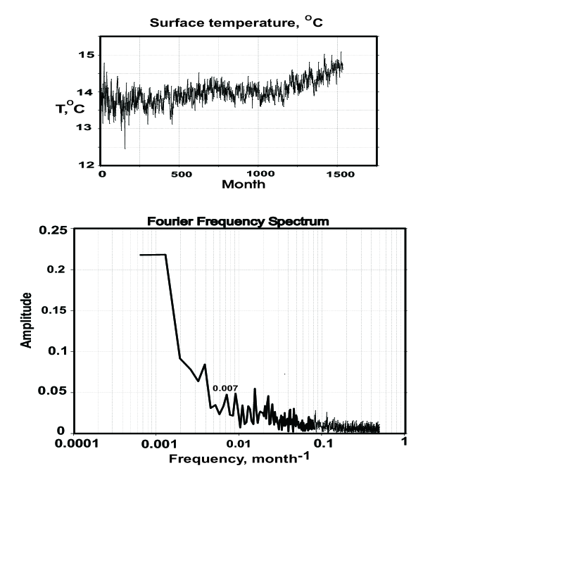
The long-term oscillations of temperature of the order $0.1^{\circ}C$ are observed in much longer time intervals ( Haigh, 2007; ACRIM ). They are usually associated with oscillations of the total solar irradiance (TSI) which has an 11-12 year periodicity. We have analysed the frequency spectrum of temperature variations for the 1880 - 2008 time interval with the result shown in Figure 9.

Figure 9.

One can notice the small peak at 0.007 month^-1 frequency, which corresponds to $\sim$ 11-year period, coincident with the 11.87-year period of the solar cycle ( Sturrock, 2008 ). The small amplitude of the peak and its corresponding low confidence level ( 2.1 standard deviations ) is presumably determined by the small amplitudes of TSI variations ( 1.7 Wm^-2 ) and of the corresponding solar forcing ( 0.3 Wm^-2 ) together with the spread in ’11 year’ periods. We remark that the similar peak in the spectrum of land temperature variations is higher by a factor of 2, which is reasonable since the land is more sensitive to TSI ( see Figure 5 ). Interestingly, there is another peak in the frequence spectrum at 0.004 month^-1, which corresponds to a 21-year solar cycle and has much higher confidence level ( 7.1 standard deviations ). Therefore, periodic variations of the surface temperature and corresponding variations of LCC are most likely of solar or perhaps geomagnetic origin rather than CR, because the 21-year variation in the CR rate is small.

The most likely cause of the anticorrelations between LCC and MCC is the variation of convection flows of the air with temperature. The rise of the surface temperature gives rise to the growing temperature in the lower atmosphere and an upward convection flows with the corresponding rise of mean cloud heights. Since clouds in the ISCCP experiment are classified by the height of their upper borders the increase of their heights leads to the redistribution along their altitudes: some low clouds cross the 3 km border and become medium clouds. As a result, LCC decreases with rising temperature. This trend is clearly seen in Figure 7, where the rise of the Global temperature in the (a)-panel is accompanied by the fall of LCC in panel (d).

The heating of the atmosphere is a slow process. The slow updraft of the air is the cause of the time lag between the variations of the surface temperature and CC. Perhaps this time lag is the reason why the maximum of the seasonal Global temperature, which is in July ( Figure 5 ), corresponds to the maximum in the seasonal variations of LCC, which is also in the middle of the year ( Figure 4 ), in spite of their anticorrelation in the long-term scale. The slow, but steady, upward convection flow of the heated air is the possible mechanism for the magnification of small TSI variations ( $\sim 0.1\%$ ) giving rise to larger variations of cloud heights ( $\sim 0.7\%$ ). The slow fall of the low cloud top pressure is seen in Figure 10. The slope of the linear fit $b$ is definitely negative: $b=-0.148\pm 0.081$ hPa $\cdot$ year^-1. It corresponds to a rise of the mean low cloud top height by about 40m in 20 years. It is very slow but one should keep in mind that the observed mean cloud top height ( $\sim$ 2.6km at 730hPa) is only $\sim$ 600m below the border ( $\sim$ 3.2km at 680mPa) between LCC and MCC and any change in the height of clouds can cause the variation of the magnitude of LCC and MCC.

We argue that the positive correlation of CR and LCC found in Svensmark and Friis-Christensen, (1997) and Palle Bago and Butler, (2000) is not evidence for a causal connection between them, but the consequence of a parallel influence of the common source - the solar activity on CR from one side and CC the other.

Concerning the relationship between CC and ground level temperature changes, there have been a number of studies for particular regions. Data for the USA covering the period 1900 to 1990 ( Barry and Chorley, 1998 ) give roughly a total ’mean annual cloud cover’ change of -1.5% over the 11-year cycle with an associated 0.2 ${}^{\circ}C$ change in ground level temperature. A value for land higher than the Global average ( 0.1% ) is to be expected and there is no inconsistency with ’our’ value.

Similar conclusions that most of the LCC variability comes from the subtropical oceans and is most likely due to TSI variations, causing changes in lower tropospheric static stability, have been made by Kristjánsson et al. (2004).

Another aspect of the Physics behind the correlation may be related to the relationship between cloud height and cloud cover ( Cotton and Anthes, 1959 ). These workers estimate that changes of -0.3% in CC from a height of 5km ( mid MCC ) correspond to a change of +0.1 ${}^{\circ}C$ at ground level ( i.e. cloud absorption of incoming radiation dominates ). In our case a change of +0.1 ${}^{\circ}C$ at ground level corresponds to a change in LCC + MCC of -0.3%, i.e. the same result although using the whole of MCC is not really appropriate. Nevertheless, there is a similarity in the values.

5 Conclusion

We advocate a scenario for the origin of correlations between CR and LCC, based on the parallel influence of solar activity. The solar irradiance rises with the sunspot number in the middle of the solar cycle. The radiation is strongest in the tropics and subtropics. Though the relative rise of the irradiance is small, and only about 0.1%, it causes a rise of the mean surface temperature and an increase of the vertical convection flows of the heated air. The subsequent change in supersaturation of the air at different heights can cause the changes in LCC and MCC. Warm air from below 3 km rising to greater heights will cause the LCC to fall and MCC to rise. By this way the rise of convection flows leads to a considerable magnification (to $\sim$ 2%) of the effect of enhanced solar irradiance. Formulating briefly, one can say that in the maxima of the solar cycles the updraft becomes stronger and this effect is strongest in the tropics and subtropics, as well as in the southern latitude bands where there is the largest fraction of area covered by the oceans. It is well known that the variations of solar activity are followed by the variations of CR intensity at Earth; the reduction of CR intensity coincident with the reduction of LCC is therefore by no means evidence of the causal connection between these two phenomena - they correlate with each other due to their common origin - the change of solar irradiance at the Earth.

Acknowledgements

K.Kudela wishes to acknowledge the VEGA grant agency, project 2/7063/27. Erlykin A.D. expresses his deep gratitude to the John C. Taylor Charitable Foundation for financial support of this work, to the staff of Climax neutron monitor
$(http://ulysses.sr.unh.edu/NeutronMonitor/neutron_{m}on.html)$
and to E.V.Vashenyuk from Apatity neutron monitor
$(http://pgi.kolasc.net.ru/CosmicRay)$
for access to their data. He thanks also S.P.Perov for useful discussions.

6 References

ACRIM: $http://acrim.com$
Barry, R.G. and Chorley, R.J., 1998, ‘Atmosphere, Weather and Climate’, Routledge, London, New York.
Bazilevskaya, G.A., Krainev, M.B., Makhmutov, V.S., Svirzhevskaya, A.K., Svirzhevsky, N.S., Stozhkov, Yu.I., 2007, Variations of Charged Particle Fluxes in the Earth’s Troposphere, Bulletin of the Lebedev Physics Institute, $\bf{34}$ , 348.
Bazilevskaya, G.A., Usoskin, I.G., Flückiger, E.O., Harrison, R.G., Desorgher, L., Bütikofer, R., Krainev, M.B., Makhmutov, V.S., Stozhkov, Yu.I., Svirzhevskaya, A.K., Svirzhevsky, N.S. and Kovaltsov, G.A., 2008, Cosmic Ray Induced Ion Production in the Atmosphere, Space Science Reviews, $\bf{137}$ , 149.
Erlykin, A.D., Gyalai, G., Kudela, K., Sloan, T., Wolfendale, A.W., 2009, Some aspects of ionization and the cloud cover, cosmic ray correlation problem, Journal of Atmospheric and Solar-Terrestrial Physics, doi:10.1016/j.jastp.2009.03.007
Ermakov, V.I., Bazilevskaya, G.A., Pokrevsky, P.E., Stozhkov, Yu.I., Ion balance equation in the atmosphere, 1997, Journal of Geophysical Research, $\bf{102}$ (D19), 23413.
Cotton, W.R. and Anthes, R.A., 1959, ’Storm and Cloud Dynamics’, Academic Press, London.
Global Surface Temperature Anomalies:
$http://lwf.ncdc.noaa.gov/oa/climate/research/anomalies/anomalies.html$
Haigh, J.D., 2007, The Sun and the Earth Climate, Living Reviews in Solar Physics., $\bf{4}$ , 2.
Hayakawa S., 1965, ’Cosmic Ray Physics’, Monographs and Texts in Physics and Astronomy, edited by R.E.Marshak, vol.XXII, John Wiley and Sons, New York, London, Sydney, Toronto
ISCCP data were obtained from the International Satellite Cloud Climatology Project web site: http://isccp.giss.nasa.gov, maintained by the ISCCP research group at NASA Goddard Institute for Space Science Studied, New York, Rossow, W.B. and Schiffer, R.A., 1999, ’Advances in understanding clouds from ISCCP’, Bulletin of the American Meteorological Society, 80, 226
Kirkby, J., 2007, Cosmic Rays and Climate, Surveys in Geophysics, 28, 335
Kristjánsson, J.E., Kristiansen, J., and Kaas, E., 2004, Solar activity, cosmic rays and climate - an update, Advances in Space Research, 34, 407
Kristjánsson, J.E., Stjern, C.W., Stordal, F., Fjæraa, A.M., Myhre, G., Jóhansson, K., 2008, Cosmic rays, cloud condensation nuclei and clouds - a reassessment using MODIS data, Atmospheric Chemistry and Physics, 8, 7373
Kudryavtsev, I.V. and Yungner, H., 2009, Cosmic rays and variations of the concentrations of active nuclei of condensation and crystallization in the Earth’s atmosphere, Bulletin of the Russian Academy of Sciences, Physics, 73, 413
Marsh, N. and Svensmark, H., 2003, Solar Influence on Earth’s Climate, Space Science Reviews, $\bf{107}$ , 317.
Mason, B.J., 1971, ‘The Physics of Clouds’ ( Clarendon Press, Oxford ).
Palle Bago, E. and Butler, C.J., 2000, The influence of cosmic rays on terrestrial clouds and global warming, Astronomy and Geophysics. 41, 4.18.
Sloan, T. and Wolfendale A.W., 2008, Could cosmic rays cause global warming ? Environmental Research Letters. $\bf{3}$ , 024001.
Sturrock, P.A., 2008, Solar neutrino variability and its implications for solar physics and neutrino physics, arXiv/0810.2755.
Svensmark, H. and Friis-Christensen, E., 1997, Variation in cosmic ray flux and global cloud coverage - a missing link in solar-climate relationship, Journal of Atmospheric and Solar-Terrestrial Physics, $\bf{59}$ , 1225.
Svensmark, H., 2007, Cosmoclimatology: a new theory emerges, News and Reviews in Astronomy and Geophysics, $\bf{48}$ , 18
Uchaikin, V.V. and Ryzhov, V.V., 1988, ’Stochastic theory of transport of high energy particles’, Nauka, Novosibirsk ( in Russian ).
Usoskin, I.G., Gladysheva, O.G., Kovaltsov, G.A., 2004, Cosmic ray induced ionization in the atmosphere: spatial and temporal changes, Journal of Atmospheric and Solar-Terrestrial Physics, $\bf{66}$ , 1791.
WDC neutron data:
http://center.stelab.nagoya-u.ac.jp/cawses/cddvd/ob0061.html

Captions to figures

Figure 1. The temporal behavior of CR (a), Global LCC (b) and the $\chi^{2}/ndf$ value as a function of the time lag between CR and LCC curves (c). Dotted lines in (a) and (b) are the mean values and dashed lines are the 5-degree polynomial fits of the CR intensity and LCC respectively.

Figure 2. Correlation plots for variations of LCC and CR during the 22nd solar cycle: (a) long-term variations, (b) short-term variations. Dashed lines in both panels are linear regression lines, the full line in the (a)-panel is the best fit curve of $Y=a+bX^{c}$ type with coefficients $a,b,c$ indicated inside the panel. The slope $b$ of the regression line and the correlation coefficient $r$ are indicated inside both panels.

Figure 3. Left set of panels: the temporal behavior of MCC and LCC ( two upper panels ), correlation plot for their long-term and short-term variations ( two lower panels ). Right set of panels: the same as the left one, but for HCC and MCC respectively.

Figure 4. Seasonal variation of the Global MCC (a) and LCC (b).

Figure 5. The seasonal variation of the sea, land and Global temperature from ( Global Surface Temperature Anomalies ). Numbers above the curves show the fraction of the total area occupied by the sea (71%) and land (29%).

Figure 6. The temporal behavior of CR (a), LCC (b) and the correlation of their long-term variations during 22d and 23d cycles of the solar activity (c).

Figure 7. The temporal behavior of the Global surface temperature (a), HCC (b), MCC (c) and LCC (d) during 22nd and 23rd cycles of solar activity. Dotted lines in (b), (c) and (d) panels show mean values of CC for 1985-2005 period of time. The dotted line in (a) panel shows the mean temperature during the last century 1900-2000, which is equal to $13.86^{\circ}C$ . It illustrates the higher temperature in the last two decades of this period - the so called Global Warming. Dashed lines show the linear fits of the temporal behavior of the surface temperature and CC. Full lines are their 5-degree polynomial approximations.

Figure 8. The latitude dependence of CC characteristics: (a) absolute values of LCC ( open circles ), MCC ( full circles ) and HCC ( open stars ). (b) LCC, MCC and HCC correlations with CR ( Climax ). Notations are the same as in (a). (c) The sensitivity of MCC to LCC ( open circles ) and their correlation coefficient ( full circles ).

Figure 9. Temporal behavior of the surface temperature in 1880-2005 years ( upper panel ) and its Fourier frequency spectrum of the global temperature for this time range ( lower panel ). The peak at 0.007 month^-1 corresponds to $\sim$ 11-year period coincident with 11.87 year solar cycle ( Sturrock, 2008 ).

Figure 10. Temporal behavior of the LCC top pressure, fitted by linear ( dotted line ) and 5-degree polynomial ( full line ) approximations.