Stable indications of relic gravitational waves in Wilkinson Microwave Anisotropy Probe data and forecasts for the Planck mission

Abstract

The relic gravitational waves are the cleanest probe of the violent times in the very early history of the Universe. They are expected to leave signatures in the observed cosmic microwave background anisotropies. We significantly improved our previous analysis zbg of the 5-year WMAP $TT$ and $TE$ data at lower multipoles $\ell$. This more general analysis returned essentially the same maximum likelihood (ML) result (unfortunately, surrounded by large remaining uncertainties): the relic gravitational waves are present and they are responsible for approximately $20\%$ of the temperature quadrupole. We identify and discuss the reasons by which the contribution of gravitational waves can be overlooked in a data analysis. One of the reasons is a misleading reliance on data from very high multipoles $\ell$, another - a too narrow understanding of the problem as the search for $B$-modes of polarization, rather than the detection of relic gravitational waves with the help of all correlation functions. Our analysis of WMAP5 data has led to the identification of a whole family of models characterized by relatively high values of the likelihood function. Using the Fisher matrix formalism we formulated forecasts for Planck mission in the context of this family of models. We explore in details various ‘optimistic’, ‘pessimistic’ and ‘dream case’ scenarios. We show that in some circumstances the $B$-mode detection may be very inconclusive, at the level of signal-to-noise ratio $S/N=1.75$, whereas a smarter data analysis can reveal the same gravitational wave signal at $S/N=6.48$. The final result is encouraging. Even under unfavourable conditions in terms of instrumental noises and foregrounds, the relic gravitational waves, if they are characterized by the ML parameters that we found from WMAP5 data, will be detected by Planck at the level $S/N=3.65$.

I Introduction

A complete cosmological theory is supposed to explain not only the present state of the observed Universe (see, for example, cosm ), but also its early dynamical behaviour and possibly its birth zg . Our present state $P$ is characterized by approximate large-scale homogeneity and isotropy within a patch of the size $l_{p}\approx 10^{3}l_{H}\approx 10^{31}{\rm cm}$ (see last paper in zg ) and the averaged energy density $\rho_{p}c^{2}$ of all sorts of matter in this patch $\rho_{p}=3H_{0}^{2}/8\pi G\approx 10^{-29}{\rm g}/{\rm cm}^{3}$, where $H_{0}$ is the present day Hubble parameter and $l_{H}=c/H_{0}\approx 10^{28}{\rm cm}$. The limits of applicability of the currently available theories are set by the Planck density $\rho_{\rm Pl}=c^{5}/G^{2}\hbar\approx 10^{94}{\rm g}/{\rm cm}^{3}$ and the Planck size $l_{\rm Pl}=(G\hbar/c^{3})^{1/2}\approx 10^{-33}{\rm cm}$. One can imagine that the embryo Universe was created by a quantum-gravity (or by a ‘theory-of-everything’) process. The emerging classical configuration was probably characterized by the near-Planckian energy density and size. The total energy, including gravity, was likely to be zero then, and remains zero now.

The problem is that this hypothesis requires further assumptions. The arising classical configuration can not reach the present state $P$ if it expands all the time according to the usual laws of radiation-dominated and matter-dominated evolution. By the time the Universe (i.e. the patch of approximate homogeneity and isotropy) has reached the size $l_{p}$, its energy density would have dropped to the level many orders of magnitude lower than the required $\rho_{p}$. Therefore, the newly born Universe needs a primordial kick before it can join the pathway of normal radiation-dominated expansion. The kick should allow the size of the patch to increase by about 33 orders of magnitude without losing too much of the energy density of whatever substance that was there, or maybe even slighly increasing this energy density at the expense of the energy density of the gravitational field.

The relic gravitational waves gr74 are necessarily generated by a strong variable gravitational field of the very early Universe. They are the cleanest probe of what was happening during the violent times of the initial kick. Specifically, the quantum-mechanical Schrödinger evolution transformes the initial no-particle (vacuum) state of the gravitational waves into a multiparticle (strongly squeezed vacuum) state. Under certain additional conditions, the same holds true for other degrees of freedom of the gravitational field (metric) perturbations, including those representing the density perurbations. As a result, the patch of homogeneity and isotropy will necessarily be augmented by primordial cosmological perturbations of quantum-mechanical origin. This process is called the superadiabatic, or parametric, amplification; for a recent review of the subject, see the last paper in gr74 .

As before (see zbg and references there), we are working with

$$ds^{2}=-c^{2}dt^{2}+a^{2}(t)(\delta_{ij}+h_{ij})dx^{i}dx^{j}=a^{2}(\eta)[-d\eta^{2}+(\delta_{ij}+h_{ij})dx^{i}dx^{j}]$$

and the Fourier-expanded gravitational field (metric) perturbations

$$h_{ij}(\eta,{\bf x})=\frac{\mathcal{C}}{(2\pi)^{3/2}}\int_{-\infty}^{+\infty}\frac{d^{3}{\bf n}}{\sqrt{2n}}\sum_{s=1,2}\left[\stackrel{{\scriptstyle s}}{{p}}_{ij}({\bf n})\stackrel{{\scriptstyle s}}{{h}}_{n}(\eta)e^{i{\bf n}\cdot{\bf x}}\stackrel{{\scriptstyle s}}{{c}}_{\bf n}+\stackrel{{\scriptstyle s~{}*}}{{p_{ij}}}({\bf n})\stackrel{{\scriptstyle s~{}*}}{{h_{n}}}(\eta)e^{-i{\bf n}\cdot{\bf x}}\stackrel{{\scriptstyle s~{}{\dagger}}}{{c_{\bf n}}}\right].$$ (1)

The polarization tensors $\stackrel{{\scriptstyle s}}{{p}}_{ij}({\bf n})$ ($s=1,2$) describe either the two transverse-traceless components of gravitational waves (gw), or the scalar and longitudinal-longitudinal components of density perturbations (dp). Assuming the initial vacuum state of participating perturbations, the resulting metric power spectra $h^{2}(n,\eta)$ are given by

$$\langle 0|h_{ij}(\eta,{\bf x})h^{ij}(\eta,{\bf x})|0\rangle=\int\limits_{0}^{\infty}\frac{dn}{n}~{}h^{2}(n,\eta),~{}~{}~{}~{}~{}h^{2}(n,\eta)\equiv\frac{\mathcal{C}^{2}}{2\pi^{2}}n^{2}\sum_{s=1,2}|\stackrel{{\scriptstyle s}}{{h}}_{n}(\eta)|^{2},$$ (2)

where the mode functions $\stackrel{{\scriptstyle s}}{{h}}_{n}(\eta)$ are taken either from gw or dp equations, and $\mathcal{C}=\sqrt{16\pi}l_{\rm Pl}$ for gravitational waves and $\mathcal{C}=\sqrt{24\pi}l_{\rm Pl}$ for density perturbations.

The numerical levels and shapes of the generated power spectra are determined by the strength and variability of the gravitational ‘pump’ field. The simplest assumption about the initial kick is that its entire duration can be described by a single power-law scale factor gr74

$$a(\eta)=l_{o}|\eta|^{1+\beta},$$ (3)

where $l_{o}$ and $\beta$ are constants, $\beta<-1$. Then, the generated primordial metric power spectra (for wavelengths longer than the Hubble radius at that time) have the universal power-law dependence on the wavenumber $n$:

$$h^{2}(n)\propto n^{2(\beta+2)}.$$ (4)

It is common to write these metric power spectra separately for gw and dp:

$$h^{2}(n)~{}({\rm gw})=B_{t}^{2}n^{n_{t}},~{}~{}~{}~{}~{}h^{2}(n)~{}({\rm dp})=B_{s}^{2}n^{n_{s}-1}.$$ (5)

In the case of power-law scale factors (3) (or piece-wise power-law scale factors), the equations for metric perturbations representing gravitational waves and density perturbations are exactly the same Grishchuk1994 . Therefore, according to the theory of quantum mechanical generation of cosmological perturbations Grishchuk1994 , the spectral indices are approximately equal, $n_{s}-1=n_{t}=2(\beta+2)$, and the amplitudes $B_{t},B_{s}$ are of the order of magnitude of the ratio $H_{i}/H_{\rm Pl}$, where $H_{i}\sim c/l_{o}$ is the characteristic value of the Hubble parameter during the kick. (An initial kick driven by a scalar field is usually associated with inflation.) In what follows, we are using the numerical code CAMB CAMB and related notations for gw and dp power spectra adopted there:

$$P_{t}(k)=A_{t}(k/k_{0})^{n_{t}},~{}~{}P_{s}(k)=A_{s}(k/k_{0})^{n_{s}-1},$$ (6)

where $k_{0}=0.002$Mpc^-1.

There is no doubt that the metric perturbations with wavelengths greater than the Hubble radius in the times of recombination do exist. Indeed, it is known for long time gz78 that it is precisely this sort of long-wavelength metric perturbations that provide the main contribution to the lower multipoles, starting from $\ell=2$, of the Cosmic Microwave Background (CMB) temperature anisotropies. The very existence of CMB anisotropies at lower $\ell$’s smoot ; wmap5 testifies to the existence of such long-wavelength perturbations. They are likely to be the perturbations of quantum-mechanical origin.

The assumption of a single power-law index $\beta$ is the simplest and easiest to analyze, but it is too strong. It has the consequence that one and the same spectral index describes the interval of 30 orders of magnitude of wavelengths in the primordial power spectra. In reality, as it appears from our CMB analysis below, even at the span of 2 orders of magnitude in terms of wavelengths the spectral index $n_{s}$ is likely to be somewhat different. We will discuss this point in more detail in the text of this paper.

We start (Sec. II) with a significant improvement of our previous analysis zbg of the 5-year Wilkinson Microwave Anisotropy Probe (WMAP5) $TE$ data at $\ell\leq 100$ LAMBDA . In contrast to zbg , we work directly with both $TT$ and $TE$ datasets and impose no restrictions on the (constant) perturbation parameters $A_{t},A_{s},n_{t},n_{s}$, except $n_{s}-1=n_{t}$ which is implied by the theory of quantum-mechanical generation. We work with the quadrupole ratio $R$

$$R\equiv\frac{C_{\ell=2}^{TT}({\rm gw})}{C_{\ell=2}^{TT}({\rm dp})}$$ (7)

and the remaining two free parameters $A_{s},n_{s}$. This more general analysis returns essentially the same as before zbg maximum likelihood (ML) values: $R=0.229$ and $n_{s}=1.086$, with approximately the same as before uncertainties. We demonstrate that the data at the multipole $\ell=2$ (dubbed “anomalously low” in the literature) are not to be blamed for these determinations. After removal of this data point altogether, the ML values do not change much. These improvements and cross-checks make more stable and robust our conclusion zbg that the WMAP5 data do contain a hint of presence of relic gravitational waves.

In Sec. III and Sec. IV we show in detail how relic gravitational waves can be overlooked in CMB data analysis. In Sec. III we concentrate on one of the reasons, which is the attempt of placing the ever “tighter” constraints on gravitational waves by using the data from high $\ell$’s of CMB and large-scale structure surveys. These data have nothing to do with gravitational waves and they can mislead the identification of gw contribution. We show that even the use of CMB data from the adjacent interval $101\leq\ell\leq 220$, where the role of gravitational waves is already small, is dangerous. We defer to Sec. IV a detailed discussion of another recipe to overlook the relic gravitational waves. This is the wide-spread ‘obsession’ with the detection of $B$-modes, rather than the detection of relic gravitational waves with the help of all available observational CMB channels.

The prospects of observing relic gravitational waves by the already deployed Planck satellite planck are analysed in great detail in Sec. IV. We adopt improved evaluations of foregrounds remove1 , foreground3 , cmbpol and instrumental noises. The main thrust of the section is the comparison of the performances of various combinations of observational channels: $TT+TE+EE+BB$, $TT+TE+EE$, and $BB$ alone. We discuss different models of the foregrounds and their subtraction, individual ‘optimistic’, ‘pessimistic’ and ‘dream case’ scenarios, as well as complications in the data analysis itself. The final conclusions are formulated not only for the model characterized by the set of ML parameters derived from the WMAP5 data, but also for the whole class of models characterized by the high values of the 3-parameter likelihood function. We show that there exists plenty of situations where the results from the $BB$ channel alone are inconclusive, whereas a smarter data analysis can reveal a significant detection. For other approaches to observing relic gravitational waves in the CMB temperature and polarization anisotropies see PolnarevKeating ; Pagano2007 .

The good news is that even under unfavorable conditions, the Planck satellite will see the relic gw signal (assuming that it has the WMAP5 maximum likelihood value $R=0.229$) at a better than 3$\sigma$ level. Furthermore, we believe that the methods and evaluations of this paper can also be used in ground-based and balloon-borne experiments BICEP ; quad ; Clover ; QUITE ; EBEX ; SPIDER ; keating2009 .

At the end of the introduction, it is important to stress that the current thinking in this area of science is greatly influenced by inflationary understanding of quantum mechanics and relativity: “Quantum fluctuations, usually observed only on microscopic scales, were stretched to astronomical sizes and promoted to cosmic significance as the seeds of large scale structure” dod , “the superluminal expansion of space during inflation stretched these scales outside of the horizon” baumann , “Inflation…stretched space…and promoted microscopic quantum fluctuations to perturbations on cosmological scales. Inflation makes detailed predictions…” EPIC , and so on.

Indeed, inflationary views on physics have translated into inflationary observational predictions. They are encapsulated in the formula for the predicted scalar metric power spectrum of density perturbations $P_{s}\approx P_{t}/\epsilon$, which is divergent at small $\epsilon$ ($\epsilon\equiv-{\dot{H}}/H^{2}$, $\epsilon=0$ in the standard inflation), and the detailed ‘tensor-to-scalar’ ratio $r$ ($r\equiv P_{t}/P_{s}$):

$$r=16\epsilon=-8n_{t}.$$ (8)

The widely quoted limits on $r$, $r<0.22$ ($95\%$ C.L.) wmap5 were derived from the likelihood function for $r$. The analysis has resulted in the maximum likelihood value $r_{ML}=0$. Since $P_{t}\approx(H_{i}/H_{\rm Pl})^{2}\neq 0$ and $r_{ML}=0$, one has to decide whether the most likely values of density perturbations $P_{s}$ responsible for the data collected and analyzed by the WMAP team are infinitely large, or inflationary predictions are wrong. The existing and planned data analyses are usually based on the enforced (incorrect) inflationary relation $r=-8n_{t}$; the final physical conclusions are formulated in terms of constraints imposed on the (possibly non-existent) scalar field, and so on (see, for example, wmap5 , EG ).

As for the quantity $r$, there is no doubt that, in general, the inflationary theory can predict for $r$ everything what one can possibly ask for (for a review, see baumann and references there). But the most advanced inflationary theories, operating with warped D-brane inflation kachru , baummc , D3-brane inflation in warped throats st , string theory inflation kl , etc., either “allow a very low tensor amplitude $r\ll 10^{-4}$”, or lead to the conclusion that “D3-brane inflation in Calabi-Yau throats, or in most tori, cannot give rise to an observably-large primordial tensor signal”, or to the conclusion that $r\approx 10^{-24}$ and the “existing models of string theory inflation do not predict a detectable level of tensor modes”. These conclusions make the search for the inflationary gravitational waves (i.e. relic gravitational waves as presented by inflationists) a senseless enterprise.

Obviously, in this paper, we are not using the inflationary theory and its observational predictions. (These predictions are based on the inflationary hat-trick of extracting arbitrarily large scalar metric perturbations $P_{s}$ out of vacuum fluctuations of the scalar field. For a more detailed criticism of inflationary theory, see last papers in gr74 and zg .)

II Improved evaluation of relic gravitational waves from WMAP $TT$ and $TE$ data

II.1 Likelihood functions and summary of the previous results

Relic gravitational waves compete with density perturbations in generating CMB temperature and polarization anisotropies at relatively low multipoles $\ell\lesssim 100$. For this reason we focus on the WMAP data at $\ell\leq 100$. As before zbg , we use the symbols $C_{\ell}^{TT}$, $C_{\ell}^{TE}$, $C_{\ell}^{EE}$, $C_{\ell}^{BB}$ for CMB power spectra and $D_{\ell}^{TT}$, $D_{\ell}^{TE}$, $D_{\ell}^{EE}$, $D_{\ell}^{BB}$ for their estimators. In this section we ignore the $B$-mode of polarization because WMAP puts only upper limits on it.

The variables $D_{\ell}^{TT}$, $D_{\ell}^{TE}$ and $D_{\ell}^{EE}$ obey the Wishart probability density function (pdf) zbg ; wishart3 ; wishart1 ; wishart2

$$f(D_{\ell}^{TT},D_{\ell}^{TE},D_{\ell}^{EE}) = \left\{\frac{1}{4(1-{\rho_{\ell}^{2}})({\sigma_{\ell}^{T}}{\sigma_{\ell}^{E}})^{2}}\right\}^{n/2}\frac{n^{3}({x}{y}-{z}^{2})^{(n-3)/2}}{\pi^{1/2}\Gamma(n/2)\Gamma((n-1)/2)}$$ (9)

$$\times \exp\left\{-\frac{1}{2(1-{\rho_{\ell}^{2}})}\left(\frac{{x}}{(\sigma_{\ell}^{T})^{2}}+\frac{{y}}{(\sigma_{\ell}^{E})^{2}}-\frac{2{\rho_{l}}{z}}{{\sigma_{\ell}^{T}}{\sigma_{\ell}^{E}}}\right)\right\},$$

where $f_{\rm sky}$ is the sky-cut factor, $f_{\rm sky}=0.85$ for WMAP and $f_{\rm sky}=0.65$ for Planck, and $n=(2\ell+1)f_{\rm sky}$ is the number of effective degrees of freedom at multipole $\ell$. $\Gamma$ is the $Gamma$-function. This pdf contains the variables $D_{\ell}^{XX^{\prime}}$ ($XX^{\prime}=TT,TE,EE$) in quantities ${x}\equiv n(D_{\ell}^{TT}+N_{\ell}^{TT})$, ${y}\equiv n(D_{\ell}^{EE}+N_{\ell}^{EE})$, ${z}\equiv nD_{\ell}^{TE}$. The information on the power spectra $C_{\ell}^{XX^{\prime}}$ is contained in quantities

$${\sigma_{\ell}^{T}}=\sqrt{C_{\ell}^{TT}+N_{\ell}^{TT}},~{}\sigma_{\ell}^{E}=\sqrt{C_{\ell}^{EE}+N_{\ell}^{EE}},~{}{\rho_{\ell}}=\frac{C_{\ell}^{TE}}{\sqrt{(C_{\ell}^{TT}+N_{\ell}^{TT})(C_{\ell}^{EE}+N_{\ell}^{EE})}},$$

where $N_{\ell}^{TT}$ and $N_{\ell}^{EE}$ are the total noise power spectra.

We are mostly interested in $TT$ and $TE$ data, so we shall work with the joint pdf for $D_{\ell}^{TT}$ and $D_{\ell}^{TE}$. This pdf is derived from (9) by integrating over the variable $D_{\ell}^{EE}$. The resulting pdf has the form

$$f(D_{\ell}^{TT},D_{\ell}^{TE})=n^{2}{x}^{\frac{n-3}{2}}\left\{2^{1+n}\pi\Gamma^{2}(\frac{n}{2})(1-\rho_{\ell}^{2})(\sigma_{\ell}^{T})^{2n}(\sigma_{\ell}^{E})^{2}\right\}^{-\frac{1}{2}}$$

$$\times\exp\left\{\frac{1}{1-\rho^{2}_{\ell}}\left(\frac{{\rho_{\ell}}{z}}{{\sigma_{\ell}^{T}}{\sigma_{\ell}^{E}}}-\frac{{z}^{2}}{2x{(\sigma_{\ell}^{E})^{2}}}-\frac{{x}}{2{(\sigma_{\ell}^{T})^{2}}}\right)\right\}.$$ (10)

In order to estimate parameters, such as $R$, $A_{s}$, $n_{s}$, from observations one seeks the maximum of the likelihood function. The likelihood function is the pdf in which the data (estimates $D_{\ell}^{XX^{\prime}}$) are known while the parameters are unknown. Up to a normalization constant, the likelihood function is

$$\mathcal{L}\propto\prod_{\ell}f(D_{\ell}^{TT},D_{\ell}^{TE})$$

for $\ell=2,\cdot\cdot\cdot,\ell_{max}$. It can be rewritten as

$$-2\ln\mathcal{L}=\sum_{\ell}\left\{\frac{1}{1-\rho^{2}_{\ell}}\left(\frac{{z}^{2}}{x{(\sigma_{\ell}^{E})^{2}}}+\frac{{x}}{{(\sigma_{\ell}^{T})^{2}}}-\frac{{2\rho_{\ell}}{z}}{{\sigma_{\ell}^{T}}{\sigma_{\ell}^{E}}}\right)+\ln\left((1-\rho_{\ell}^{2})(\sigma_{\ell}^{T})^{2n}(\sigma_{\ell}^{E})^{2}\right)\right\}+C,$$ (11)

where the constant $C$ is chosen to make the maximum value of $\mathcal{L}$ equal to 1.

Our previous analysis zbg was based on the background $\Lambda$CDM cosmological model as derived in wmap5old . In addition to the relation $n_{t}=n_{s}-1$, the perturbation parameters $A_{s},A_{t}$ were restricted by the observational condition $\ell(\ell+1)C_{\ell}^{TT}/2\pi|_{\ell=10}=840~{}\mu{\rm K}^{2}$. One more restriction was supplied by the phenomenological relation $n_{s}(R)=0.96+0.35R-0.07R^{2}$ which indirectly took into account the data on $TT$ anisotropies. The remaining free parameter $R$ was subject to the likelihood analysis. This analysis was directly using the 5-year WMAP $TE$ data at multipoles $2\leq\ell\leq 100$ LAMBDA . The noise power spectra $N_{\ell}^{TT}$, $N_{\ell}^{EE}$ were obtained from the information posted at LAMBDA and were presented as graphs in zbg (Fig. 6).

The likelihood procedure has resulted in $R=0.240^{+0.291}_{-0.225}$ (68.3% C.L.). For the ML value $R=0.240$, the imposed restrictions have produced the full set of perturbation parameters:

$$R=0.240,~{}~{}n_{s}=1.040,~{}~{}A_{s}=2.034\times 10^{-9},~{}~{}A_{t}=0.960\times 10^{-9}$$ (12)

and $n_{t}=0.040$. A shift of the parameter $R$ within its confidence interval would automatically produce a change in other parameters too.

In order to avoid any association with inflationary predictions, we are not using the parameter $r$. However, if $r$ is defined as $r\equiv A_{t}/A_{s}$ (definition used by the WMAP team) without implying inflationary formulas (8), then one can establish a relation between $R$ and $r$ which depends on the background cosmological model and spectral indices Rossetta . We derived this relation numerically. For a rough comparison of results one can use $r\approx 2R$.

II.2 Revised analysis of the WMAP5 data

In this paper, the previous approach zbg is improved in two main aspects. First, we work directly with both datasets, $TT$ and $TE$. Second, in the likelihood procedure all three parameters $R,A_{s},n_{s}$ are kept free. (We tried to include $n_{t}$ as a free parameter, but this did not change the results except increasing uncertainties around the ML values.)

As before, the WMAP5 estimates for $D_{\ell}^{TT}$, $D_{\ell}^{TE}$ at multipoles $\ell\leq\ell_{max}=100$ are taken from LAMBDA . The noise power spectra $N_{\ell}^{TT}$, $N_{\ell}^{EE}$ are the same as derived in zbg (Fig. 6). Numerical evaluations of the CMB power spectra are performed with the help of CAMB code CAMB .

The adopted background model is the best-fit $\Lambda$CDM cosmology wmap5 (ApJS version) with parameters

$$\begin{array}[]{c}\Omega_{b}h^{2}=0.02267^{+0.00058}_{-0.00059},~{}\Omega_{c}h^{2}=0.1131\pm 0.0034,\\ \Omega_{\Lambda}=0.726\pm 0.015,~{}\tau_{\rm reion}=0.084\pm 0.016,~{}h=0.705\pm 0.013.\end{array}$$ (15)

In numerical calculations, we use the central values of these parameters.

Applying the Markov Chain Monte Carlo (MCMC) method (see, for example, mcmc1 ; mcmc2 ), we probe the likelihood function (11) by 10,000 samples and determine the position of its maximum in 3-dimensional space $R,A_{s},n_{s}$. The parameters of our best-fit model, i.e. the maximum likelihood (ML) values of the perturbation parameters, are found to be

$$R=0.229,~{}~{}~{}n_{s}=1.086,~{}~{}~{}A_{s}=1.920\times 10^{-9}$$ (16)

and $n_{t}=0.086$. Obviously, these are only the coordinates of the maximum in the parameter space. There are many neighbouring points with almost equally large values of the likelihood $\mathcal{L}$. It is difficult to visualize the 3-dimensional region around the maximum, so in Fig. 1 we show the projection of the 10,000 sample points on the 2-dimensional planes $R-n_{s}$ and $R-A_{s}$.

The color of an individual point in Fig. 1 signifies the value of the 3-dimensional likelihood of the corresponding sample. The projections of the maximum (16) are shown by a black $+$. The samples with relatively large values of the likelihood (red, yellow and green colors) are concentrated along the curve, which projects into relatively straight lines (at least, up to $R\approx 0.5$):

$$n_{s}=0.98+0.46R,~{}~{}~{}~{}~{}A_{s}=(2.27-1.53R)\times 10^{-9}.$$ (17)

These combinations of the parameters $R,n_{s},A_{s}$ produce roughly equal responses in the CMB power spectra. The best-fit model (16) is a particular point on these lines, $R=0.229$. We will be using this one-parameter family of models (17) in our study of the detection abilities of the Planck mission in Section IV.

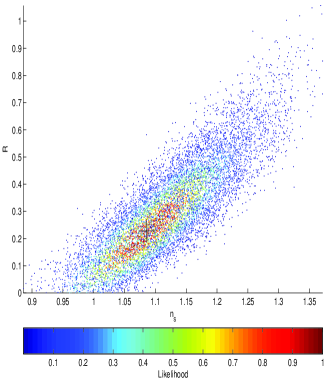
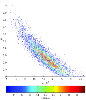
Figure 1: The projection of 10,000 samples of the 3-dimensional likelihood function onto the $R-n_{s}$ (left panel) and $R-A_{s}$ (right panel) planes. The black $+$ indicates the parameters listed in (16).

Before comparing the new and old results, it is instructive to explore the marginalized 2-dimensional and 1-dimensional distributions. The marginalized distribution over a parameter is the integral of the likelihood function over that parameter. By integrating $\mathcal{L}$ (11) over $A_{s}$ or $n_{s}$ we derive 2-dimensional likelihoods in $R-n_{s}$ or $R-A_{s}$ spaces. Then we apply the standard procedure of finding the maxima and confidence contours.

In the left panel of Fig. 2 we show the ML point (marked by a red $\times$) and the $68.3\%$ and $95.4\%$ confidence contours (red solid lines) in the $R-n_{s}$ plane. The 2-parameter maximum is located at

$$R=0.203,~{}~{}n_{s}=1.082.$$ (18)

In the same panel we show 2-dimensional confidence contours as given by the WMAP team wmap5 . We transferred their contours originally plotted in $r-n_{s}$ plane to our $R-n_{s}$ plane using the numerical relation between $R$ and $r$. Their contours are based either on the assumed constancy of the spectral index $n_{s}$ throughout all the explored multipoles (black dashed curves), or on a simple running of $n_{s}$, $n_{s}(k)=n_{s}(k_{0})+\frac{dn_{s}}{d\ln k}\ln(\frac{k}{k_{0}})$ (blue dash-dotted curves).

In the right panel of Fig. 2 we show the ML point (marked by a red $\times$) and the $68.3\%$ and $95.4\%$ confidence contours (red solid lines) in the $R-A_{s}$ plane. The 2-parameter maximum is located at

$$R=0.211,~{}~{}A_{s}=1.877\times 10^{-9}.$$ (19)

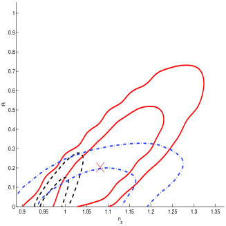
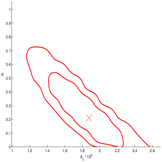
Figure 2: The ML points (red $\times$) and the $68.3\%$ and $95.4\%$ confidence contours (red solid lines) for 2-dimensional likelihoods: $R-n_{s}$ (left panel) and $R-A_{s}$ (right panel). In the left panel, the WMAP confidence contours are also shown for comparison.

Integrating the likelihood function $\mathcal{L}$ (11) over two parameters ($A_{s}$, $n_{s}$), ($A_{s}$, $R$) or ($R$, $n_{s}$), we arrive at 1-dimensional distributions for $R$, $n_{s}$ or $A_{s}$, respectively. We plot these distributions in Fig. 3. The ML values of these parameters and their $68.3\%$ confidence intervals are given by

$$R=0.266\pm 0.171,~{}~{}n_{s}=1.107^{+0.087}_{-0.070},~{}~{}A_{s}=(1.768^{+0.307}_{-0.245})\times 10^{-9}.$$ (20)

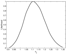
Figure 3: 1-dimensional likelihoods for $R$ (left), $n_{s}$ (middle) and $A_{s}$ (right).

Comparing the old, Eq. (12), and new, Eqs. (16), (18), (19), (20), results, one can conclude the following. First, all the results are close to each other and deviate little around the rigorous 3-dimensional ML values (16). Second, the parameter $R$ persistently indicates a significant amount of relic gravitational waves, even if with a considerable uncertainty. The $R=0$ hypothesis (no gravitational waves) appears to be away from the $R=0.229$ model at about $1\sigma$ interval, or a little more, but not yet at a significantly larger distance. Third, the spectral indices $n_{s},n_{t}$ persistently point out to the ‘blue’ shape of the primordial spectra, i.e. $n_{s}>1,n_{t}>0$, in the interval of wavelengths responsible for the analyzed multipoles $\ell\leq\ell_{max}=100$. This puts in doubt the (conventional) scalar fields as a possible driver for the initial kick, because the scalar fields cannot support $\beta>-2$ in Eq. (3) and, consequently, $n_{s}>1,n_{t}>0$ in Eq. (6).

II.3 Quadrupole data and extrapolation of the ML model to higher multipoles

It is known quadrupole1 that the actually observed quadrupole $D_{\ell=2}^{TT}$ has anomalously low value in comparison with the usually plotted graphs of the best-fit CMB power spectra. Since our results prefer a somewhat ‘blue’ primordial spectrum, the natural question arises whether the low value of the quadrupole is not the reason entirely responsible for our evaluation. In order to answer this question we have conducted the likelihood analysis without using the observed data points $D_{\ell=2}^{TT}$ and $D_{\ell=2}^{TE}$. We found that even this drastic measure of complete removal of these data points does not change our results qualitatively. The parameters of the maximum likelihood model modify to $R=0.190$, $n_{s}=1.067$ and $A_{s}=1.993\times 10^{-9}$. This is one more evidence of the stability of indications on the presence of relic gravitational waves in the WMAP5 CMB data.

As was already stressed in the paper, we analyze only those WMAP5 data where one can expect to find relic gravitational waves, that is, in the range $2\leq\ell\leq 100$. Therefore, the parameters (16) apply only to wavelengths responsible for that range. We will show in Sec. III that it can be misleading to try to constrain gravitational waves by the data outside this interval of multipoles, as the spectral indices may change. Nevertheless, it is interesting to see what kind of CMB power spectra the ML model (16) generates, if the spectral indices are assumed fixed at their values (16) throughout all the relevant wavelengths.

In Fig. 4, we show these extrapolated $TT$ and $TE$ power spectra built on the ML parameters (16). One can see that these spectra are not too far away from the “no gravitational waves” spectra advocated by the WMAP team. As one could expect, the somewhat ‘blue’ spectral index $n_{s}$ in (16) makes the extrapolated spectra positioned somewhat above the WMAP5 spectra at very large multipoles.

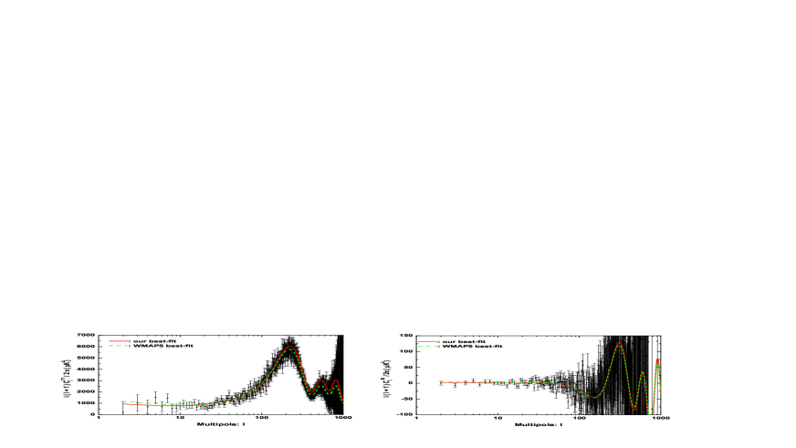
Figure 4: The unbinned WMAP5 $TT$ (left panel) and $TE$ (right panel) data LAMBDA , along with their uncertainties due to noises and statistics. The red solid lines show the ML model (16) extrapolated with constant spectral indices to high multipoles. For comparison, the dashed green line shows the WMAP5 best-fit “no gravitational waves” model.

III How relic gravitational waves can be overlooked in the likelihood analysis of $TT$ and $TE$ data

With all the reservations already stated, our results are markedly different from the WMAP5 conclusions wmap5 . The WMAP team has found no evidence for gravitational waves and arrived at a red spectral index $n_{s}=0.96$. The WMAP findings are symbolized by black dashed and blue dash-dotted contours in Fig. 2. It is important to understand the reasons for these disagreements.

Two differences in data analysis have already been mentioned. We restrict our analysis to multipoles $\ell\leq 100$, whereas the WMAP team uses the data at all multipoles up to $\ell\sim 1000$ keeping spectral indices constant. We use the relation $n_{t}=n_{s}-1$ implied by the theory of quantum-mechanical generation of cosmological perturbations, whereas the WMAP team uses the inflationary ‘consistency relation’ $r=-8n_{t}$ which automatically sends $r$ to zero when $n_{t}$ approaches zero. There could be some discrepencies in treating the noises, but we think we effectively followed zbg the WMAP prescriptions. After several trials, we came to the conclusion (with heavy heart, as Einstein used to say) that it is the assumed constancy of spectral indices in a broad spectrum that is mostly responsible for the disagreement, and it should be abandoned. The constancy of $n_{s}$ over the vast region of wavenumbers, or possibly a simple running of $n_{s}$, is a usual assumption in a number of works wmap5 , othergroups ; wishart3 .

In order to understand the impact of higher multipole data, we first probed the likelihood function and estimated the parameters from the data in the range of multipoles $101\leq\ell\leq 220$. The procedure was exactly the same as was used in the analysis of $2\leq\ell\leq 100$ data. The maximum of the 3-parameter likelihood function was found at $n_{s}=0.923$, $R=0.022$ and $A_{s}=2.65\times 10^{-9}$, that is, at a distinctly ‘red’ spectral index $n_{s}$. The 2-dimensional marginalized distribution $R-n_{s}$ (analogous to the left panel in Fig. 2) is also different. It is shown in the left panel of Fig. 5. The large uncertainty surrounding $R=0.022$ reflects the fact that, at these multipoles, the contribution of relic gravitational waves becomes very small. It is the density perturbations that play dominant role here, and at higher multipoles. The 1-dimensional marginalized distribution for $n_{s}$ (analogous to the middle panel in Fig. 3) is shown in the left panel of Fig. 6. This distribution gives $n_{s}=0.948^{+0.052}_{-0.061}$ ($68.3\%$ C.L.). Obviously, this value of $n_{s}$ is significantly smaller than the one in Eq. (20), and the two evaluations do not overlap in 1$\sigma$ confidence interval. This is a clear indication that the spectral index $n_{s}$ can hardly be treated as one and the same constant throughout all the wavelengths responsible for $2\leq\ell\leq 100$ and $101\leq\ell\leq 220$ intervals.

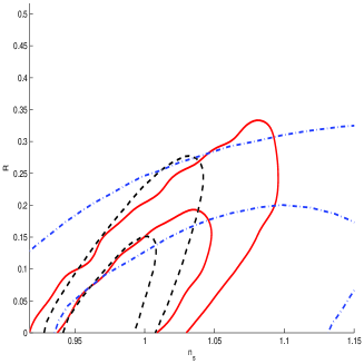
Figure 5: Same evaluations as in the left panel in Fig. 2, but derived from WMAP5 $TT+TE$ data in the interval $101\leq\ell\leq 220$ (left panel), and in the interval $2\leq\ell\leq 220$ (right panel). WMAP5 contours wmap5 are shown for comparison.

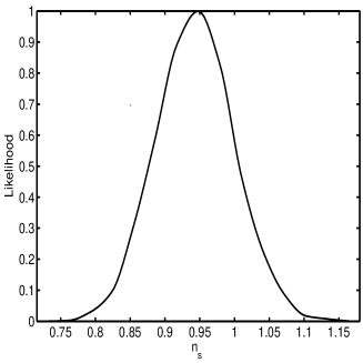
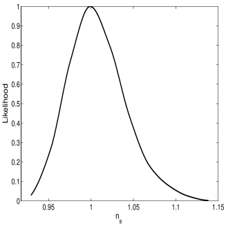
Figure 6: 1-dimensional likelihood for $n_{s}$ derived from WMAP5 $TT+TE$ data in the interval $101\leq\ell\leq 220$ (left panel), and in the interval $2\leq\ell\leq 220$ (right panel).

As one could expect, exactly the same analysis of the whole interval $2\leq\ell\leq 220$ from the position of constant $n_{s}$ leads to the ML values which are intermediate between evaluations at the intervals $2\leq\ell\leq 100$ and $101\leq\ell\leq 220$ separately. The 3-parameter likelihood analysis applied to WMAP5 $TT+TE$ data in the interval $2\leq\ell\leq 220$ has resulted in the ML values $n_{s}=0.973$, $R=0.019$ and $A_{s}=2.39\times 10^{-9}$. As expected, the ML value $n_{s}=0.973$ is in between the ML values $n_{s}=1.086$ and $n_{s}=0.923$ from the two adjacent intervals of $\ell$. The 2-dimensional marginalized constraints are shown in the right panel of Fig. 5. In comparison with the left panel, the uncertainty contours are much closer to the WMAP5 evaluations. The 1-dimensional marginalized distribution for $n_{s}$ is shown in the right panel of Fig. 6. It gives $n_{s}=0.998^{+0.036}_{-0.029}$ ($68.3\%$ C.L. ). Again, this is the intermediate value of $n_{s}$ in comparison with evaluations from the two intervals of $\ell$ separately. Our evaluation of $n_{s}$ from the data in the interval $2\leq\ell\leq 220$ still gives a little bit higher value of $n_{s}$ than $n_{s}=0.96$ found by the WMAP team, but presumably the remaining difference is accounted for by the multipoles $\ell>220$ and other data sets that were included in the WMAP derivation.

One can see now why the inclusion of data from $\ell>100$ is dangerous. Although these data have nothing to do with gravitational waves, they bring $n_{s}$ down. If one assumes that $n_{s}$ is one and the same constant at all $\ell$’s, this additiosnal ‘external’ information about $n_{s}$ affects uncertainty about $R$ and brings $R$ down. This is clearly seen, for example, in the left panel of Fig. 2. The localization of $n_{s}$ near, say, the line $n_{s}=0.96$ would cross the solid red contours along that line and would enforce lower, or zero, values of $R$. However, as we have shown above, the $n_{s}$ is sufficiently different even at the span of the two neighbouring intervals of $\ell$’s that we discussed. These considerations as for how relic gravitational waves can be overlooked have general significance and will be applicable to any CMB data and data analysis.

IV Forecasts for the Planck mission

Now, that Planck satellite planck is launched, it is important to see in detail how the maximum likelihood model (16) found from WMAP5 data, as well as neighbouring models defined by Eq. (17), will fare in the less noisy Planck data. In our previous work zbg , we restricted our consideration to only two separate information channels, namely to $TE$ and $BB$ correlation functions. We took into account only one frequency channel $143\rm{GHz}$ and its instrumental noise. We replaced the unknown level of residual foregrounds and systematics by the increased total noise in the $BB$ channel, calling it a ‘realistic’ $BB$ channel. On the data analysis side, we performed the likelihood analysis with a single parameter $R$, assuming that other parameters $A_{s}$, $n_{s}$ and $n_{t}=n_{s}-1$ are known, as long as they are related to $R$ by the imposed restrictions.

In this paper, we study the detection abilities of Planck in a much more comprehensive manner. First, we consider all available information channels, i.e. $TT$, $TE$, $EE$ and $BB$ correlation functions, and their combinations. Second, in evaluating the instrumental noises, we take into account all the Planck’s frequency channels (either three, or even all seven). Third, we include in the total noise the residual foreground contamination from the synchrotron and dust emissions, and introduce the ‘pessimistic’ case when the foregrounds are not removed at all while the nominal instrumental noise in the $BB$ channel is increased by a factor of 4. Finally, we search not only for a single parameter $R$, but where the computational resources allow, we evaluate the uncertainties for $R$ arising in the procedure of joint determination of all three unknown parameters $R$, $n_{s}$, $A_{s}$ from a given set of observational data.

IV.1 The signal-to-noise ratio in the measurement of $R$

IV.1.1 The noise power spectra and the definition of $S/N$

Surely, in the focus of our attention is the detection of relic gravitational waves. Their CMB contribution is parameterized by $R$. To quantify the detection ability of a CMB experiment, we introduce the signal-to-noise ratio zbg

$$S/N\equiv R/\Delta R,$$ (21)

where the numerator is the true value of the parameter $R$ (or its ML value, or the input value in a numerical simulation) while $\Delta R$ in the denominator is the expected uncertainty in determination of $R$ from the data.

In formulating the observational forecasts, it is common to use the Fisher matrix formalism. We outline its main features in Appendix A. The uncertainty $\Delta R$, for a given $R$, depends on noises, statistics of the searched for CMB signal (which is random in itself), and the number of parameters subject to evaluation from a given dataset. The instrumental and foreground noises comprise the total effective noise power spectra $N_{\ell}^{XX^{\prime}}$ which enter the Fisher matrix (29) and its element $F_{RR}$, Eq. (31), as well as the element ${\left(F^{-1}\right)_{RR}}$ of the inverse matrix. Depending on the number of sought after parameters, one calculates $\Delta R$ either according to Eq. (30) or according to Eq. (32).

The noise power spectra $N_{\ell}^{XX^{\prime}}$ are explained in Appendix B. We ignore the cross-correlated noises, i.e. when $X\neq X^{\prime}$, so we are working only with $N_{\ell}^{XX}$. The instrumental characteristics of all seven frequency channels planck (we mark them by symbol $i=1,\cdot\cdot\cdot,7$) are listed in Table 1 of Appendix B, where LFI means Low Frequency Instrument and HFI High Frequency Instrument. Following planck we treat only three frequency channels $100$GHz, $143$GHz and $217$GHz as providing CMB data, whereas other channels are supposed to be used for determining the foregrounds. However, in Section IV.3 we study the improvements that would arise if one could use all seven frequency channels for CMB analysis. It is seen from (33), that three channels are better than one, and seven channels are better than three.

The residual foreground noise $N_{{\rm fg},\ell}^{XX}(i)$ adds to the instrumental noise $N_{{\rm ins},\ell}^{XX}(i)$ and increases the total noise $N_{\ell}^{XX}$ (33). We neglect the effect of foregrounds in $TT$ channel because this noise is small in comparison with the signal bennett . The foreground contamination cannot be neglected in polarization channels. The synchrotron and dust emissions are expected to be the dominant hindrances in the Planck frequency range foreground3 ; foreground2 ; cmbpol-fore . The charecteristics of the accepted foreground models are listed in Appendix B. In what follows, we are using the more severe Dust A model, whereas the more favorable Dust B model is considered only in Section IV.3.

The ways of mitigating the foreground contamination are discussed in a number of papers remove1 ; remove2 ; remove3 ; remove4 ; remove5 ; remove6 . In this paper, we take a phenomenological approach and quantify the residual noise by the factor $\sigma^{\rm fg}$ (see foreground3 and Appendix B) which multiplies the model power spectra $C_{S,\ell}^{XX}(i)$, $C_{D,\ell}^{XX}(i)$ of the synchrotron (S) and dust (D) emissions. We consider three cases, $\sigma^{\rm fg}=1$ (no foreground removal), $\sigma^{\rm fg}=0.1$ ($10\%$ foreground residual noise) and $\sigma^{\rm fg}=0.01$ ($1\%$ foreground residual noise). In order to gauge the worst case scenario, we consider also the ‘pessimistic’ case, where $\sigma^{\rm fg}=1$ and $N_{{\rm ins},\ell}^{BB}(i)$ at each frequency $\nu_{i}$ is 4 times larger than the values listed in Table 1. This increased noise is meant to mimic the situation where it is not possible to get rid of various systematic effects systematics , the $E$-$B$ mixture ebmixture , cosmic lensing lensing , etc. which all affect the $BB$ channel.

To illustrate the expected total noise, including the different levels of foreground contamination, we show in Fig. 7 the total noise power spectrum $N_{\ell}^{BB}$ calculated according to Eq.(33). For reference, the black curve shows the power spectrum $C_{\ell}^{BB}$ for the maximum likelihood model with $R=0.229$ (see Eq. (16)) extrapolated up to $\ell=1000$. It is seen from the graphs that the role of foregrounds is restricted to relatively small multipoles $\ell\lesssim 20$. For higher multipoles, the total noise $N_{\ell}^{BB}$ is dominated by the instrumental noise and does not depend on $\sigma^{\rm fg}$. It can also be seen from Fig. 7 that it is only for small values of $\sigma^{\rm fg}$, i.e. in the case when the foreground contamination is significantly suppressed, that the signal $C_{\ell}^{BB}$ will be greater than the noise $N_{\ell}^{BB}$ at lowest multipoles. Thus, even in the case of small $\sigma^{\rm fg}$, the Planck’s $BB$ channel will be mostly sensitive to gravitational waves in the epoch of reionization. For larger values of $\sigma^{\rm fg}$, the relative contribution of lower multipoles to the total $S/N$ is diminished, signifying the overall reduction of $S/N$. In this case, the main contribution to $S/N$ comes from higher multipoles $\ell\gtrsim 20$ and $S/N$ will ultimately be limited by the level of instrumental noise.

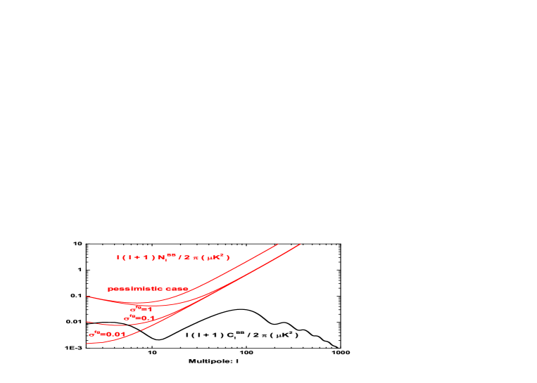
Figure 7: The total noise power spectrum $\ell(\ell+1)N_{\ell}^{BB}/2\pi$ in comparison with the $BB$ power spectrum $\ell(\ell+1)C_{\ell}^{BB}/2\pi$ for the model (16) with $R=0.229$.

IV.1.2 The analysis of the family of models (17), including the $ML$ model (16)

The set of maximum likelihood parameters (16) is the best set among the ‘almost equally good’ sets, defined by (17). In a sense, Eq. (17) is our theoretical prediction, based on the analysis of WMAP5 data, of the best viable perturbation models. This family of models is the subject of the Fisher matrix analysis below. With all the noises $N_{\ell}^{XX}$ defined by (33) and all the power spectra $C_{\ell}^{XX^{\prime}}$ calculable from the family parameters (17), we have enough ammunition to find the quantities (29).

We start from the idealized situation, where only one parameter $R$ is considered unknown and therefore the uncertainty $\Delta R$ can be found from (30). All the information channels, $TT$, $TE$, $EE$, $BB$, are used in the calculation of $F_{RR}$, Eq. (31). The results for $S/N$ are plotted in the left panel of Fig. 8. Four options are depicted, $\sigma=0.01,0.1,1$ and the pessimistic case.

The results for the benchmark model (16) are given by the intersection points along the vertical line $R=0.229$. The signal to noise is high, $S/N=9.35$, if the foregrounds can be removed to the level $\sigma^{\rm fg}=0.01$, and $S/N$ decreases to $S/N=8.80$, $S/N=7.72$, $S/N=6.48$ for $\sigma^{\rm fg}=0.1$, $\sigma^{\rm fg}=1$, and the pessimistic case, respectively. In all these cases, the $S/N$ is impressively large. A value of $R$ down to $R=0.03$ can be measured with $S/N=2$ in the optimistic scenario $\sigma^{\rm fg}=0.01$, whereas $S/N>2$ is achieved for $R>0.064$ in the pessimistic case. Typically, the optimistic scenario gives $S/N$ about 1.5 times larger than the pessimistic case, with the disparity growing larger for smaller values of $R$.

As one could expect, the uncertainty $\Delta R$ grows and $S/N$ decreases in the realistic situation, when all unknown parameters $R$, $n_{s}$ and $A_{s}$ are supposed to be evaluated from one and the same dataset. In this case, $\Delta R$ should be calculated according to (32). Again, calculating $\left(F^{-1}\right)_{RR}$, we take into account all the information channels $TT$, $TE$, $EE$, $BB$. The results for $S/N$ are presented in the right panel of Fig. 8. For the benchmark model (16), the signal-to-noise ratios are smaller than in the left panel: $S/N=6.69,~{}6.20,~{}5.15$ if $\sigma^{\rm fg}=0.01,~{}0.1,~{}1$, respectively.

However, the good news is that even in the pessimistic case one gets $S/N>2$ for $R>0.11$, and the Planck satellite will be capable of seeing the ML signal $R=0.229$ at the level $S/N=3.65$.

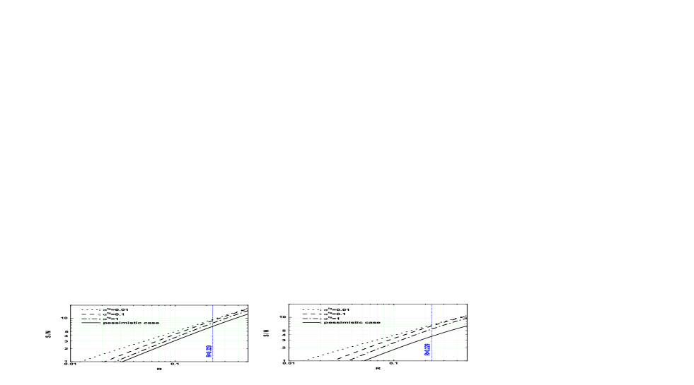
Figure 8: The $S/N$ as a function of $R$. In the left panel, the uncertainty $\Delta R$ is calculated according to Eq. (30), whereas in the right panel it is calculated according to Eq. (32).

IV.2 Contributions of individual information channels and individual multipoles to the total $S/N$

The evaluations in Sec. IV.1.2 assume that all the correlation functions, $TT+TE+EE+BB$, are taken into account and all the relevant multipoles $\ell$ participate in the summations. The total $S/N$ can only be worse if something is missing either in the information channels or in the accessible multipoles. In order to gain further insight into the detection ability of Planck, it is instructive to make a break-up of $S/N$ over combinations of information channels and multipoles. It is unclear how to do this in the case of Eq. (32), but it is relatively easy to do this in the case of Eq. (30). We will limit ourselves to this latter case which is sufficient for the purpose of illustration.

The $S/N$ from Eq. (21), together with $\Delta R$ from Eq. (30), can be rewritten as

$$(S/N)^{2}=R^{2}F_{RR},$$ (22)

The $F_{RR}$ from Eq. (31) is a simple sum over multipoles $\ell$, so the $(S/N)^{2}$ in (22) can be decomposed into individul $\ell$-contributions

$$(S/N)^{2}=\sum_{\ell}(S/N)_{\ell}^{2}.$$ (23)

Each individul $(S/N)_{\ell}^{2}$ depends on all information channels, with the $BB$-channel factored out, as was infixed from the very beginning in the form of Eq. (26),

$$(S/N)_{\ell}^{2} = \frac{R^{2}(2\ell+1)f_{\rm sky}}{2\left({\cal C}_{\ell}^{TT}{\cal C}_{\ell}^{EE}-({\cal C}_{\ell}^{TE})^{2}\right)^{2}}\times\left\{({\cal C}_{\ell}^{TT})^{2}\frac{\partial{\cal C}_{\ell}^{EE}}{\partial R}\frac{\partial{\cal C}_{\ell}^{EE}}{\partial R}+({\cal C}_{\ell}^{EE})^{2}\frac{\partial{\cal C}_{\ell}^{TT}}{\partial R}\frac{\partial{\cal C}_{\ell}^{TT}}{\partial R}\right.$$ (24)

$$+2\left({\cal C}_{\ell}^{TT}{\cal C}_{\ell}^{EE}+\left({\cal C}_{\ell}^{TE}\right)^{2}\right)\frac{\partial{\cal C}_{\ell}^{TE}}{\partial R}\frac{\partial{\cal C}_{\ell}^{TE}}{\partial R}+2\left({\cal C}_{\ell}^{TE}\right)^{2}\frac{\partial{\cal C}_{\ell}^{TT}}{\partial R}\frac{\partial{\cal C}_{\ell}^{EE}}{\partial R}$$

$$\left.+4{\cal C}_{\ell}^{TE}\left({\cal C}_{\ell}^{TT}\frac{\partial{\cal C}_{\ell}^{EE}}{\partial R}+{\cal C}_{\ell}^{EE}\frac{\partial{\cal C}_{\ell}^{TT}}{\partial R}\right)\frac{\partial{\cal C}_{\ell}^{TE}}{\partial R}\right\}+\frac{R^{2}(2\ell+1)f_{\rm sky}}{2({\cal C}_{\ell}^{BB})^{2}}\frac{\partial{\cal C}_{\ell}^{BB}}{\partial R}\frac{\partial{\cal C}_{\ell}^{BB}}{\partial R}.$$

The natural break-up of Eq. (24) into combinations of the information channels is $TT+TE+EE+BB$, $TT+TE+EE$ and $BB$ alone.

IV.2.1 Signal to noise ratio for different combinations of information channels

Using either all terms in Eq. (24), or everything without $BB$, or $BB$ alone, we calculate $(S/N)^{2}$, Eq. (23), for three combinations of channels: $TT+TE+EE+BB$, $TT+TE+EE$ and $BB$ alone. The $(S/N)^{2}$ for the first (full) combination is the sum of $(S/N)^{2}$ for the other two. Since the foreground removal is a major concern, we separate the results into four groups - $\sigma^{\rm fg}=0.01,~{}0.1,~{}1$ and the pessimistic case. The results for $S/N$ are shown in Fig. 9 in four panels. Certainly, the (red) lines marked by $TT+TE+EE+BB$ in four panels are the same lines that are shown in the left panel of Fig. 8 for the corresponding case. The copy of the line representing the optimistic scenario in the upper left panel, i.e. $TT+TE+EE+BB$ together with $\sigma^{\rm fg}=0.01$, is shown by a (black) dashed line in other panels as a reminder of what can be achieved in the optimistic scenario.

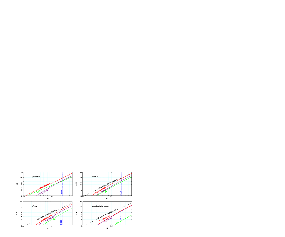
Figure 9: The $S/N$ for different combinations of the information channels, $TT+TE+EE+BB$, $TT+TE+EE$ and $BB$.

Surely, the combination $TT+TE+EE+BB$ is more sensitive than any of the other two, $TT+TE+EE$ and $BB$ alone. For example, in the case $\sigma^{\rm fg}=0.1$, the use of all channels provides $S/N$ which is $\sim 50\%$ greater than $BB$ alone and $\sim 30\%$ greater than $TT+TE+EE$. The situation is even more peculiar in the pessimistic case. The ML model (16) can be barely seen through the popular $B$-modes alone, because the $BB$ channel gives only $S/N=1.75$, whereas the use of all channels can provide a confident detection with $S/N=6.48$.

Comparing $TT+TE+EE$ with $BB$, one can see that the first method is better than the second, except in the case when $\sigma^{\rm fg}=0.01$ and $R$ is small ($R<0.16$). In the pessimistic case, the role of the $BB$ channel is so small that the $TT+TE+EE$ method provides essentially the same sensitivity as all channels $TT+TE+EE+BB$ together.

Considering the $S/N$ for $BB$ alone, it is worth noting that since the $BB$ channel is not sensitive to $A_{s}$ and $n_{s}$ the uncertainty (32) reduces to (30). Therefore, although the results for $BB$ channel alone, shown in Fig. 9, were derived under the assumption of a single unknown parameter $R$, they apply also in the general case when all three parameters, $R$, $n_{s}$, $A_{s}$, are supposed to be determined from the temperature and polarization data.

IV.2.2 Multipole decomposition of $S/N$

It is seen from Eq. (23) the the total $(S/N)^{2}$ is a sum over $\ell$-contributions $(S/N)_{\ell}^{2}$ given by Eq. (24). Formally, the sum can extend to large $\ell$’s, but a smaller $R$-signal and larger noises make the large $\ell$’s irrelevant anyway. We go up to $\ell_{max}=100$.

In Fig. 10 and Fig. 11 we plot the quantity $(S/N)_{\ell}^{2}$ as a function of $\ell$ for different combinations of information channels and different $\sigma^{\rm fg}$, including the pessimistic case. Fig. 10 presents the multipole decomposition for the ML model (16) with $R=0.229$, while Fig. 11 sorts out the $R=0.05$ model characterized by $S/N=3$ for $\sigma^{\rm fg}=0.01$ (see left panel in Fig. 8). Note the differences in scaling on vertical axes in Fig. 10 and Fig. 11.

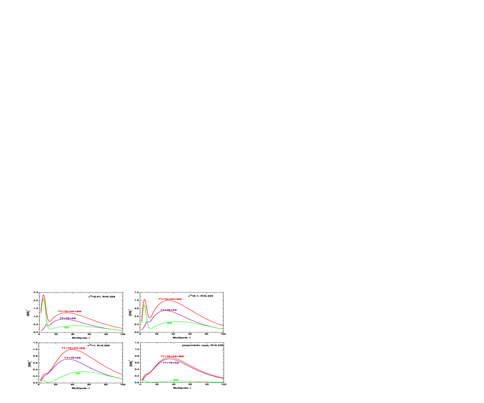
Figure 10: The individual $(S/N)_{\ell}^{2}$ as functions of $\ell$ for different combinations of information channels and different levels of foreground contamination. Calculations are done for the ML model (16) with $R=0.229$.

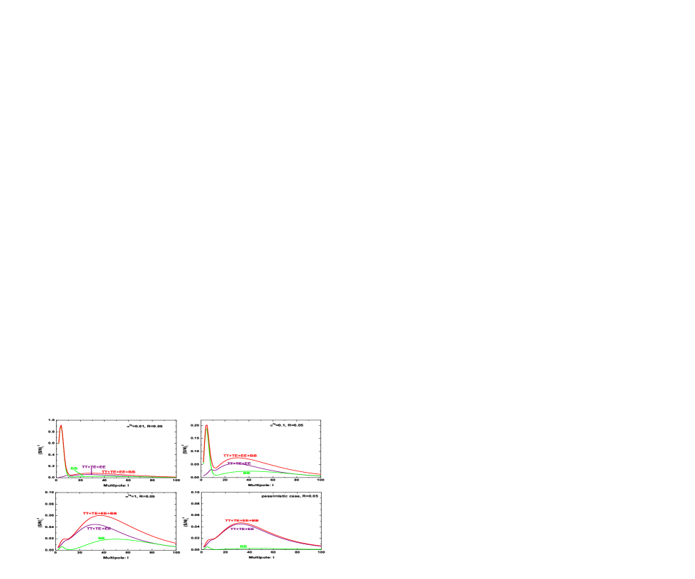
Figure 11: The same illustrations as in Fig. 10, but for the model (17) with $R=0.05$.

Both figures show again that a very deep foreground cleaning, $\sigma^{\rm fg}=0.01$, makes the very low (reionization) multipoles $\ell\simeq 10$ the major contributors to the total $(S/N)^{2}$, and mostly from the $BB$ channel. This is especially true for the lower-$R$ model $R=0.05$. However, for large $\sigma^{\rm fg}=0.1,~{}1$, and especially in the pessimistic case (see the lower right panels in Figs. 10 and 11), the role of the $BB$ channel becomes very small at all $\ell$’s. These detailed illustrations in terms of multipole decomposition of $(S/N)^{2}$ are of course fully consistent with the integrated results of Sec. IV.2.1.

At the same time, as Figs. 10 and 11 illustrate, the $\ell$-decomposition of $(S/N)^{2}$ for $TT+TE+EE$ combination depends only weakly on the level of $\sigma^{\rm fg}$. Furthermore, in this method, the signal-to-noise curves generally peak at $\ell\sim(20-50)$. Therefore, it will be particularly important for Planck mission to avoid excessive noises in this region of multipoles.

IV.3 On the possibilities to get a better value for $S/N$

So far, the $S/N$ was calculated using the generally quoted realistic assumptions about instrumental and environmental noises. It appears that some reserves to get better values for $S/N$ still exist. These possibilities seem speculative but worth exploring. First, one may find a way of using the outputs of all seven frequency channels (listed in Table 1) for the CMB analysis. The summation over $i=1,\cdot\cdot\cdot,7$, instead of $i=1,2,3$, would effectively reduce the instrumental part of noise in $N_{\ell}^{XX}$ (33). Second, we may be lucky and the Dust B model turns out to be correct one, rather than the more severe Dust A model. This would reduce the foreground part of noise in $N_{\ell}^{XX}$ (33).

Below, we consider three possibilities of these improvements in $S/N$. Namely, the use of 3 frequency channels and the validity of Dust B model, the use of 7 frequency channels and the validity of Dust A model, and the ‘dream case’ of using all 7 frequency channels in the conditions of validity of Dust B model. For these three options, we do exactly the same calculations that were done in Sec. IV.1.2 and depicted in Fig. 8. The left panel in Fig. 8 translates into the three upper panels in Fig. 12, and the right panel in Fig. 8 translates into the three lower panels in Fig. 12.

Certainly, one sees considerable improvements in $S/N$, especially in the ‘dream case’ scenario (upper right and lower right panels in Fig. 12). For example, concentrating on the solid line in the lower right panel, one finds that the ML model (16) with $R=0.229$ would be detectable at the level $S/N=5.11$, instead of $S/N=3.65$ that we found in the right panel in Fig. 8. This would significantly increase the chance of observing relic gravitational waves with the help of the Planck mission.

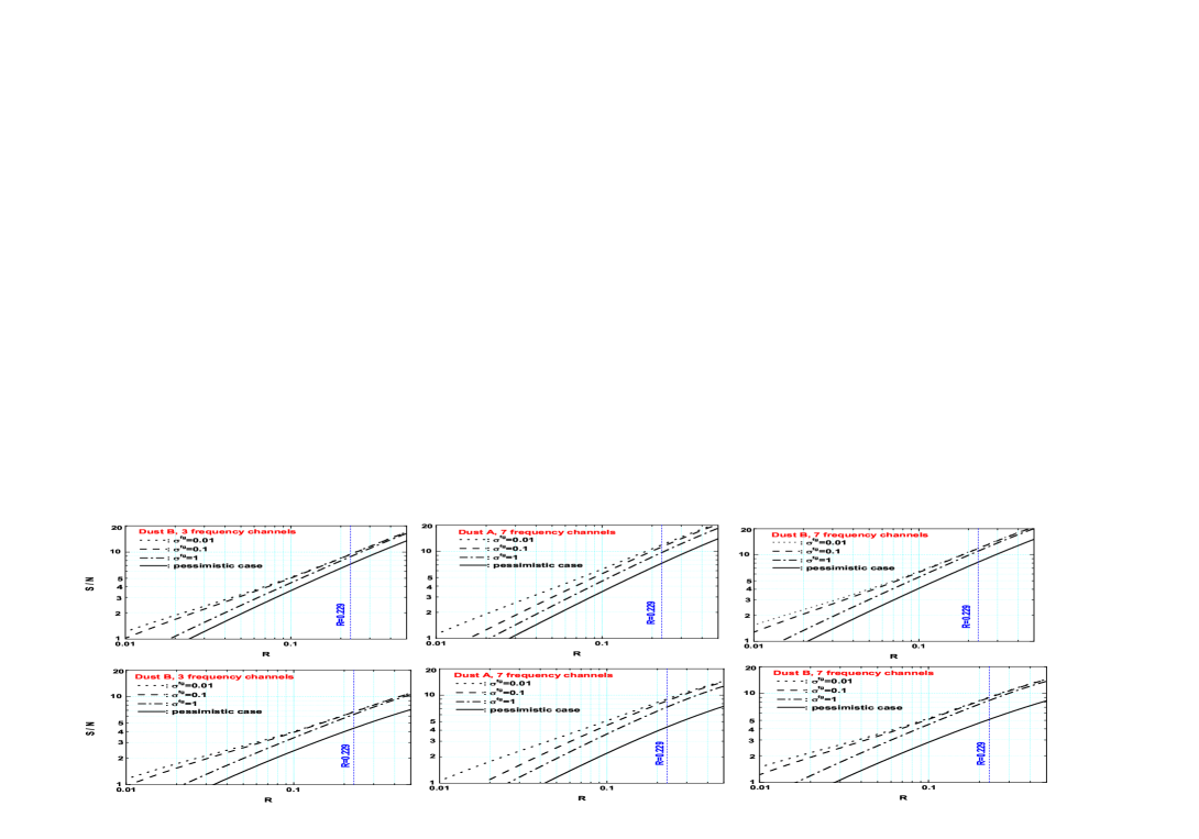
Figure 12: The improved values of $S/N$. The three upper panels should be compared with the left panel in Fig. 8, and the three lower panels with the right panel in Fig. 8.

V Conclusions

Being in the possession of general theoretical confidence that the relic gravitational waves are expected to be present in the observed CMB anisotropies, we improved our previous analysis of WMAP5 data and made comprehensive forecasts for the Planck mission.

The improvements in the analysis of the WMAP5 $TT$ and $TE$ observations made our approach more general and stable. The new analysis avoids phenomenological relations and restrictions, and deals directly with the complete 3-parameter likelihood function and its marginalizations. The result of this analysis is very close to the previous one: the maximum likelihood value for the quadrupole ratio $R$ is $R=0.229$. This means that approximately 20% of the temperature quadrupole is caused by gravitational waves and 80% by density perturbations. Although the uncertainties due to large noises are still large, this result can be regarded as an indication of the presence of relic gravitational waves in the lower $\ell$ CMB anisotropies (we would love to call it a suspected detection, but we resist this temptation).

We identify and study in detail the reasons by which the contribution of relic gravitational waves can be overlooked in a data analysis. One of the reasons is the unjustified reliance on constancy of the spectral index $n_{s}$ and the inclusion of data from very high multipoles $\ell$. Another reason - a too narrow understanding of the problem as the search for $B$-modes of polarization, rather than the detection of relic gravitational wave with the help of all correlation functions.

Our forecasts for Planck are also based on our analysis of WMAP5 observations. We identify the whole family of models, that is, the sets of perturbation parameters $R$, $n_{s}$, $A_{s}$, which are almost as good as the unique model with the maximum likelihood, $\mathcal{L}=1$, set of parameters $R=0.229,n_{s}=1.086,A_{s}=1.920\times 10^{-9}$. For the same observational data, these sets of parameters return reasonably high numerical values of the likelihood function $\mathcal{L}$. We formulate our forecasts for this family of models, which is characterized by observationally preferred sets of parameters, rather than choosing the models and parameters at random and blindly. Our forecasts, based on the Fisher matrix techniques, refer to achievable signal-to-noise ratios $S/N$. We analyze many sources of noise and explore various ‘optimistic’, ‘pessimistic’ and ‘dream case’ scenarios. We discuss the circumstances in which the $B$-mode detection is very inconclusive, at the level $S/N=1.75$, whereas a smarter data analysis reveals the same gravitational wave signal at $S/N=6.48$.

The very encouraging final result is that, even under unfavourable conditions in terms of instrumental noises and foregrounds, the relic gravitational waves, if they are characterized by the WMAP5 maximum likelihood value $R=0.229$, will be detected by Planck at the level $S/N=3.65$.

Acknowledgements

Wen Zhao is partially supported by Chinese NSF Grants No. 10703005 and No. 10775119.

Appendix A Fisher information matrix in the CMB analysis

In the CMB data analysis, the general form of the likelihood function, up to a normalization constant, is

$$\mathcal{L}\propto\prod_{\ell}f(D_{\ell}^{TT},D_{\ell}^{TE},D_{\ell}^{EE},D_{\ell}^{BB}).$$ (25)

Since $D_{\ell}^{BB}$ is independent of the rest of variables $D_{\ell}^{TT}$, $D_{\ell}^{TE}$, $D_{\ell}^{EE}$ zbg , the likelihood function factorizes,

$$\mathcal{L}\propto\prod_{\ell}f(D_{\ell}^{TT},D_{\ell}^{TE},D_{\ell}^{EE})f(D_{\ell}^{BB}).$$ (26)

The pdf $f(D_{\ell}^{TT},D_{\ell}^{TE},D_{\ell}^{EE})$ is the Wishart distribution given by Eq. (9), whereas $f(D_{\ell}^{BB})$ is the $\chi^{2}$ distribution:

$$f(D_{\ell}^{BB})=\frac{nV^{(n-2)/2}e^{-V/2}}{2^{n/2}\Gamma(n/2)(C_{\ell}^{BB}+N_{\ell}^{BB})},$$ (27)

where $V$ is $V\equiv n(D_{\ell}^{BB}+N_{\ell}^{BB})/(C_{\ell}^{BB}+N_{\ell}^{BB})$. The likelihood function is a function of the sought after parameters $s_{i}$, which in our case are perturbation parameters $A_{t}$, $A_{s}$, $n_{t}$, $n_{s}$. They enter the likelihood function through their presence in the power spectra $C_{\ell}^{XX^{\prime}}$. The $BB$ part of $\mathcal{L}$ depends only on $A_{t}$ and $n_{t}$. We have reduced the set of parameters $s_{i}$ to $R$, $n_{s}$, $A_{s}$.

The Fisher information matrix is a measure of the width and shape of the likelihood function, as a function of the parameters, around its maximum. The Fisher matrix formalism is used for estimation of the accuracy with which the parameters of interest can be found from the data fisher1 ; fisher2 . The elements of the matrix are expectation values of the second derivatives of logarithm of the likelihood function with respect to $s_{i}$,

$$F_{s_{i}s_{j}}=\left.\left\langle-\frac{\partial^{2}{(\ln\cal{L}})}{\partial s_{i}\partial s_{j}}\right\rangle\right|_{{s}_{i}=\bar{s}_{i}},$$ (28)

where $\bar{s}_{i}$ are the true values of ${s}_{i}$ (i.e. values where the average of the first derivative of $\ln\cal{L}$ vanishes). The angle brackets denote the integration over the joint pdf for all $D_{\ell}^{XX^{\prime}}$.

Inserting (26) into (28), one can calculate the Fisher matrix,

$$F_{s_{i}s_{j}}=\sum_{\ell}\sum_{XX^{\prime},YY^{\prime}}\frac{\partial{C}_{\ell}^{XX^{\prime}}}{\partial s_{i}}{{\rm Cov}^{-1}(D_{\ell}^{XX^{\prime}},D_{\ell}^{YY^{\prime}})}\frac{\partial{C}_{\ell}^{YY^{\prime}}}{\partial s_{j}},$$ (29)

where ${\rm Cov}^{-1}$ is the inverse of the covariance matrix. (Result (29) coincides with Eq. (7) in fisher2 .) The non-vanishing components of the covariance matrix are given by

$${\rm Cov}(D_{\ell}^{XX},D_{\ell}^{XX}) = \frac{2}{(2\ell+1)f_{\rm sky}}(C_{\ell}^{XX}+N_{\ell}^{XX})^{2}~{}~{}~{}(X=T,E,B),$$

$${\rm Cov}(D_{\ell}^{TE},D_{\ell}^{TE}) = \frac{1}{(2\ell+1)f_{\rm sky}}[(C_{\ell}^{TE})^{2}+(C_{\ell}^{TT}+N_{\ell}^{TT})(C_{\ell}^{EE}+N_{\ell}^{EE})],$$

$${\rm Cov}(D_{\ell}^{TT},D_{\ell}^{EE}) = \frac{2}{(2\ell+1)f_{\rm sky}}(C_{\ell}^{TE})^{2},$$

$${\rm Cov}(D_{\ell}^{TT},D_{\ell}^{TE}) = \frac{2}{(2\ell+1)f_{\rm sky}}C_{\ell}^{TE}(C_{\ell}^{TT}+N_{\ell}^{TT}),$$

$${\rm Cov}(D_{\ell}^{EE},D_{\ell}^{TE}) = \frac{2}{(2\ell+1)f_{\rm sky}}C_{\ell}^{TE}(C_{\ell}^{EE}+N_{\ell}^{EE}).$$

When a particular parameter $s$ is estimated from the data, while other parameters are assumed to be known, the uncertainty in the determination of this parameter is given by $\Delta s=1/\sqrt{F_{ss}}$. However, if all parameters are estimated from the data, the uncertainty rises to $\Delta s=\sqrt{(F^{-1})_{ss}}$. The second uncertainty is always larger than the first one or equal to it.

In this work, we are mostly interested in the parameter $R$, which quantifies the contribution of relic gravitational waves to the CMB anisotropies. The definition of the signal-to-noise ratio $S/N$ in Eq. (21) requires the specification of the uncertainty $\Delta R$. If other parameters are fixed and only $R$ is derived from the data, this uncertainty is given by the matrix element $F_{RR}$,

$$\Delta R={1}/{\sqrt{F_{RR}}}.$$ (30)

Explicit expression for $F_{RR}$ follows from Eq. (29),

$$F_{RR} = \sum_{\ell}\frac{R^{2}(2\ell+1)f_{\rm sky}}{2\left({\cal C}_{\ell}^{TT}{\cal C}_{\ell}^{EE}-({\cal C}_{\ell}^{TE})^{2}\right)^{2}}\times\left\{({\cal C}_{\ell}^{TT})^{2}\frac{\partial{\cal C}_{\ell}^{EE}}{\partial R}\frac{\partial{\cal C}_{\ell}^{EE}}{\partial R}+({\cal C}_{\ell}^{EE})^{2}\frac{\partial{\cal C}_{\ell}^{TT}}{\partial R}\frac{\partial{\cal C}_{\ell}^{TT}}{\partial R}\right.$$ (31)

$$+2\left({\cal C}_{\ell}^{TT}{\cal C}_{\ell}^{EE}+\left({\cal C}_{\ell}^{TE}\right)^{2}\right)\frac{\partial{\cal C}_{\ell}^{TE}}{\partial R}\frac{\partial{\cal C}_{\ell}^{TE}}{\partial R}+2\left({\cal C}_{\ell}^{TE}\right)^{2}\frac{\partial{\cal C}_{\ell}^{TT}}{\partial R}\frac{\partial{\cal C}_{\ell}^{EE}}{\partial R}$$

$$\left.+4{\cal C}_{\ell}^{TE}\left({\cal C}_{\ell}^{TT}\frac{\partial{\cal C}_{\ell}^{EE}}{\partial R}+{\cal C}_{\ell}^{EE}\frac{\partial{\cal C}_{\ell}^{TT}}{\partial R}\right)\frac{\partial{\cal C}_{\ell}^{TE}}{\partial R}\right\}+\frac{R^{2}(2\ell+1)f_{\rm sky}}{2({\cal C}_{\ell}^{BB})^{2}}\frac{\partial{\cal C}_{\ell}^{BB}}{\partial R}\frac{\partial{\cal C}_{\ell}^{BB}}{\partial R},$$

where $\mathcal{C}_{\ell}^{XX}\equiv C_{\ell}^{XX}+N_{\ell}^{XX}$, and $\mathcal{C}_{\ell}^{TE}\equiv C_{\ell}^{TE}$.

If other parameters are being determined together with $R$, the uncertainty $\Delta R$ is given by the $RR$ element of the inverse matrix,

$$\Delta R={\sqrt{\left(F^{-1}\right)_{RR}}}.$$ (32)

The uncertainty (32) is always greater than (30) or equal to it. We use (30) and (32) for numerical evaluation of $S/N$.

Appendix B The instrumental and environmental noise power spectra

CMB experiments use several frequency channels (distinguished by the label $i$) which have specific instrumental and environmental noises at each frequency $\nu_{i}$. The optimal combination of the channels gives the total effective noise power spectrum $N_{\ell}^{XX}$ foreground3 ; cmbpol ; Bowden2004

$$[N_{\ell}^{XX}]^{-2}=\sum_{i\geq j}\left[(N_{{\rm fg},\ell}^{XX}(i)+N_{{\rm ins},\ell}^{XX}(i))(N_{{\rm fg},\ell}^{XX}(j)+N_{{\rm ins},\ell}^{XX}(j))\frac{1}{2}(1+\delta_{ij})\right]^{-1},$$ (33)

where $N_{{\rm ins},\ell}^{XX}(i)$ and $N_{{\rm fg},\ell}^{XX}(i)$ are the instrumental and residual foreground noise power spectra, respectively. The total effective noise power spectrum $N_{\ell}^{XX}$ enters the Fisher matrix (29).

In the evaluation of noise power spectra we set the window function equal to 1, which is a good approximation for the multipoles considered in this paper, $\ell\leq 220$. The instrumental characteristics of the Planck’s frequency channels are reported in Table 1 based on planck . This Table provides $N_{{\rm ins},\ell}^{XX}(i)$. As for the polarized foregrounds ($XX=EE,BB$), we focus on the synchrotron (S) and dust (D) emissions. The foreground contamination is quantified by the parameter $\sigma^{{\rm fg}}=1,~{}0.1,~{}0.01$ which multiplies the power spectra $C_{S,\ell}^{XX}(i)$, $C_{D,\ell}^{XX}(i)$ of the accepted foreground models. The smaller $\sigma^{{\rm fg}}$ the deeper cleaning. The residual foreground noise is given by foreground3

$$N_{{\rm fg},\ell}^{XX}(i)=\sum_{{f}=S,D}\left[C_{{f},\ell}^{XX}(i)\sigma^{{\rm fg}}+\mathcal{N}_{{f},\ell}^{XX}(i)\right],$$ (34)

where $\mathcal{N}_{f,\ell}^{XX}(i)$ is the noise power spectrum arising from the cleaning procedure itself in the presence of instrumental noise.

Table 1: Summary of Planck Instrumental Characteristics

Instrument Characteristic	LFI			HFI
Center Frequency [GHz]	30	44	70	100	143	217	353
Angular Resolution [FWHM arcmin]	33	24	14	10	7.1	5.0	5.0
$N_{{\rm ins},\ell}^{TT}$ [$10^{-4}\mu$K2]	27.37	26.38	27.20	3.93	1.53	3.62	33.94
$N_{{\rm ins},\ell}^{EE}$ and $N_{{\rm ins},\ell}^{BB}$ [$10^{-4}\mu$K2]	53.65	55.05	55.28	10.05	5.58	15.09	139.50

Following foreground3 ; cmbpol ; foreground2 , for the $\ell$ and $\nu_{i}$ dependences of the synchrotron and dust emissions we take

$$C_{S,\ell}^{XX}(i)=A_{S}\left(\frac{\nu_{i}}{\nu_{0}}\right)^{2\alpha_{S}}\left(\frac{\ell}{\ell_{0}}\right)^{\beta_{S}}$$ (35)

and

$$C_{D,\ell}^{XX}(i)=p^{2}A_{D}\left(\frac{\nu_{i}}{\nu_{0}}\right)^{2\alpha_{D}}\left(\frac{\ell}{\ell_{0}}\right)^{\beta_{D}^{XX}}\left[\frac{e^{h\nu_{0}/kT}-1}{e^{h\nu_{i}/kT}-1}\right]^{2}.$$ (36)

In Eq. (36), $p$ is the dust polarization fraction, estimated to be $5\%$ foreground3 , and $T$ is the temperature of the dust grains, assumed to be constant across the sky $T=18$K foreground3 . Other parameters in Eqs. (35), (36) are specified in Table 2 taken from cmbpol .

Table 2: Assumptions about foregrounds cmbpol

Parameter	Synchrotron	Dust A	Dust B
$A_{S,D}$	$4.7\times 10^{-5}$ $\mu$K2	$1.0$ $\mu$K2	$1.2\times 10^{-4}$ $\mu$K2
$\nu_{0}$	30 GHz	94 GHz	94 GHz
$\ell_{0}$	350	10	900
$\alpha$	-3	2.2	2.2
$\beta^{EE}$	-2.6	-2.5	-1.3
$\beta^{BB}$	-2.6	-2.5	-1.4

The noise term $\mathcal{N}_{f,\ell}^{XX}(i)$ ($f=S,D$) entering Eq. (34) was calculated in foreground3 ; cmbpol

$$\mathcal{N}_{f,\ell}^{XX}(i)=\frac{N_{{\rm ins},\ell}^{XX}(i)}{n_{\rm chan}(n_{\rm chan}-1)/4}\left(\frac{\nu_{i}}{\nu_{\rm ref}}\right)^{2\alpha}.$$

Here, $n_{\rm chan}$ is the total number of frequency channels used in making the foreground template map, and $\nu_{\rm ref}$ is the frequency of the reference channel. In the case of the dust, $\nu_{\rm ref}$ is the highest frequency channel included in the template making, while in the case of the synchrotron, $\nu_{\rm ref}$ is the lowest frequency channel. The value of $\alpha$ is given in Table 2 for different foreground models.

All components of noise are used in numerical calculations of the total noise (33).

References

- (1) W. Zhao, D. Baskaran and L. P. Grishchuk, Phys. Rev. D 79, 023002 (2009).
- (2) Ya. B. Zeldovich and I. D. Novikov, Structure and Evolution of the Universe (Nauka, Moscow, 1975; University of Chicago Press, Chicago, 1983); P. J. E. Peebles, Principles of Physical Cosmology (Princeton University Press, Princeton, 1993); S. Weinberg, Cosmology (Oxford University Press, New York, 2008).
- (3) Ya. B. Zeldovich, Pis’ma Zh. Eksp. Teor. Fiz. 7, 579 (1981); L. P. Grishchuk and Ya. B. Zeldovich, in Quantum Structure of Space and Time, Eds. M. Duff and C. Isham, (Cambridge University Press, Cambridge, 1982), p. 409; Ya. B. Zel’dovich, Cosmological field theory for observational astronomers, Sov. Sci. Rev. E Astrophys. Space Phys. Vol. 5, pp. 1-37 (1986) (http://nedwww.ipac.caltech.edu/level5/Zeldovich/Zel_contents.html); L. P. Grishchuk, Space Science Reviews (Springer), published online 5 May 2009 [arXiv:0903.4395].
- (4) L. P. Grishchuk, Zh. Eksp. Teor. Fiz. 67, 825 (1974) [Sov. Phys. JETP 40, 409 (1975)]; Ann. N. Y. Acad. Sci 302, 439 (1977); Pis’ma Zh. Eksp. Teor. Fiz. 23, 326 (1976) [JETP Lett. 23, 293 (1976)]; Usp. Fiz. Nauk 121, 629 (1977) [Sov. Phys. Usp. 20, 319 (1977)]; L. P. Grishchuk, Discovering Relic Gravitational Waves in Cosmic Microwave Background Radiation, in “Wheeler Book”, Eds. I. Ciufolini and R. Matzner (Springer, New York, in press) [arXiv:0707.3319].
- (5) L. P. Grishchuk, Phys. Rev. D 50, 7154 (1994).
- (6) http://camb.info/.
- (7) L. P. Grishchuk and Ya. B. Zeldovich, Astron. Zh. 55, 209 (1978) [Sov. Astron. 22, 125 (1978)].
- (8) G. F. Smoot et al., Astrophys. J. 396, L1 (1992).
- (9) E. Komatsu et al., Astrophys. J. Suppl. Ser. 180, 330 (2009).
- (10) http://lambda.gsfc.nasa.gov/.
- (11) Planck Collaboration, The Science Programme of Planck [astro-ph/0604069].
- (12) G. Efstathiou, S. Gratton and F. Paci, arXiv:0902.4803.
- (13) L. Verde, H. Peiris and R. Jimenez, J. Cosmol. Astropart. Phys. 0601, 019 (2006).
- (14) D. Baumann et al., AIP Conf. Proc. 1141, 10 (2009) (Appendix C1).
- (15) A. G. Polnarev, N. J. Miller and B. G. Keating, Mon. Not. R. Astron. Soc. 386, 1053 (2008).
- (16) L. Pagano, A. Cooray, A. Melchiorri and M. Kamionkowski, Journal of Cosmology and Astroparticle Physics 0804, 009 (2008).
- (17) B. G. Keating et al., in Polarimetry in Astronomy, edited by Silvano Fineschi, Proceedings of the SPIE, 4843 (2003).
- (18) C. Pryke et al., QUaD collaboration, arXiv:0805.1944.
- (19) A. C. Taylor, Clover Collaboration, New Astron. Rev. 50, 993 (2006).
- (20) D. Samtleben, arXiv:0806.4334.
- (21) P. Oxley et al., astro-ph/0501111.
- (22) B. P. Crill et al., arXiv:0807.1548.
- (23) H. C. Chiang et al., arXiv:0906.1181.
- (24) S. Dodelson et al., arXiv:0902.3796.
- (25) D. Baumann et al., arXiv:0811.3919.
- (26) J. Bock et al., arXiv:0906.1188.
- (27) G. Efstathiou and S. Gratton, arXiv:0903.0345.
- (28) S. Kachru et al., J. Cosmol. Astropart. Phys., 0310, 013 (2003) [hep-th/0308055].
- (29) D. Baumann and L. McAllister, Phys. Rev. D 75, 123508 (2007) [hep-th/0610285].
- (30) E. Silverstein and D. Tong, Phys. Rev. D 70, 103505 (2004) [hep-th/0310221].
- (31) R. Kallosh and A. Linde, J. Cosmol. Astropart. Phys., 0704, 017 (2007) [arXiv:0704.0647].
- (32) W. Zhao, Phys. Rev. D 79, 063003 (2009); W. Zhao and D. Baskaran, Phys. Rev. D 79, 083003 (2009).
- (33) S. Hamimeche and A. Lewis, Phys. Rev. D 77, 103013 (2008).
- (34) W. J. Percival and M. L. Brown, Mon. Not. R. Astron. Soc. 372, 1104 (2006); H. K. Eriksen and I. K. Wehus, Astrophys. J. Suppl. Ser. 180, 30 (2009).
- (35) E. Komatsu et al., arXiv:0803.0547v1.
- (36) M. S. Turner and M. White, Phys. Rev. D 53, 6822 (1996); S. Chongchitnan and G. Efstathiou, Phys. Rev. D 73, 083511 (2006).
- (37) A. Gelman, J. B. Carlin, H. S. Stern and D. B. Rubin, Bayesian Data Analysis (ACRC Press Company, Boca Raton, USA, 2004); W. R. Gilks, S. Richardson and D. J. Spiegelhalter, Markov Chain Monte Carlo in Practice (ACRC Press Company, Boca Raton, USA, 1996).
- (38) A. Lewis and S. Bridle, Phys. Rev. D 66, 103511 (2002).
- (39) M. R. Nolta et al., Astrophys. J. Suppl. Ser. 180, 296 (2009).
- (40) e.g. A. Lewis, Phys. Rev. D 78, 023002 (2008); J. Q. Xia, H. Li, G. B. Zhao and X. M. Zhang, Phys. Rev. D 78, 083524 (2008); L. P. L. Colombo, E. Pierpaoli and J. R. Pritchard, arXiv:0811.2622.
- (41) C. L. Bennett et al., Astrophys. J. Suppl. Ser. 148, 97 (2003).
- (42) M. Tucci, E. Martinez-Gonzalez, P. Vielva and J. Delabrouille, Mon. Not. R. Astron. Soc. 360, 926 (2005).
- (43) J. Dunkely et al., arXiv:0811.3915.
- (44) A. Amblard, A. Cooray and M. Kaplinghat, Phys. Rev. D 75 083508 (2007).
- (45) R. Saha, P. Jain and T. Souradeep, Astrophys. J. 645, L89 (2006); T. Ghosh, R. Saha, P. Jain and T. Souradeep, arXiv:0901.1641; P. K. Samal et al., arXiv:0903.3634.
- (46) J. Kim, P. Naselsky and P. R. Christensen, Phys. Rev. D 79, 023003 (2009).
- (47) M. Betoule et al., arXiv:0901.1056.
- (48) J. Delabrouille et al., arXiv:0807.0773.
- (49) W. Hu, M. M. Hedman and M. Zaldarriaga, Phys. Rev. D 67, 043004 (2003); D. O’Dea, A. Challinor and B. R. Johnson, Mon. Not. R. Astron. Soc. 376, 1767 (2007); M. Shimon, B. Keating, N. Ponthieu and E. Hivon, Phys. Rev. D 77, 083003 (2008).
- (50) A. Lewis, A. Challinor, and N. Turok, Phys. Rev. D 65, 023505 (2001); M. L. Brown, P. G. Castro, and A. N. Taylor, Mon. Not. R. Astron. Soc. 360, 1262 (2005); A. de Oliveira-Costa and M. Tegmark, Phys. Rev. D 74, 023005 (2006).
- (51) M. Zaldarriaga and U. Seljak, Phys. Rev. D 58, 023003 (1998); W. Hu, Phys. Rev. D 62, 043007 (2000).
- (52) M. Tegmark, A. Taylor and A. Heavens, Astrophys. J. 480, 22 (1997).
- (53) M. Zaldarriaga, D. Spergel and U. Seljak, Astrophys. J. 488, 1 (1997).
- (54) M. Bowden et al., Mon. Not. R. Astron. Soc. 349, 321 (2004).