hep-th/0907.1170
FIT HE - 09-01

Kagoshima HE - 09-1

Stability of D brane Anti D brane Systems
in Confining Gauge Theories

Kazuo Ghoroku^†, ^§Akihiro Nakamura ^¶Fumihiko Toyoda

^†Fukuoka Institute of Technology, Wajiro, Higashi-ku

Fukuoka 811-0295, Japan

^§Department of Physics, Kagoshima University, Korimoto 1-21-35,

Kagoshima 890-0065, Japan

^¶School of Humanity-Oriented Science and Engineering, Kinki University,

Iizuka 820-8555, Japan

Abstract

We study the stability of a special form of D brane embedding which is regarded as a bound state of D_n and anti-D_n-brane embedded in a 10D supergravity background which is dual to a confining gauge theory. For D5 branes with $U(1)$ flux, their bound state configuration can be regarded as the baryonium vertex. For D branes of $n=6$ and 8 without the $U(1)$ flux, their bound states have been used to introduce flavor quarks in the dual supersymmetric Yang-Mills theory. In any case, it would be important to assure that they are free from tachyon instability. For all these cases, we could show their stability with respect to this point.

1 Introduction

It would be a challenging problem to make clear the deep structure of mesons, baryons and other hadrons which are the bound states of quarks. The quantum chromodynamics is well defined to solve these problems, but it is very difficult to see the non-perturbative properties of this theory. A very promising approach in this direction has been performed in the recent holographic approaches. According to the quark model, the baryons are composed of $N_{c}$ quarks combined at a vertex point, which would however not a point but has a structure and the vertex with a structure has been expressed in type IIB theory by D5-branes wrapped on $S^{5}$ in AdS${}_{5}\times S^{5}$ space-time [1, 2, 3, 4, 5, 8, 9, 10, 11, 12, 13, 14] based on the string/gauge theory correspondence [15, 16, 17]. And the baryon has been constructed as a system of fundamental strings (F-strings) corresponding to the quarks and this vertex [18, 19, 20, 21, 22, 23, 24].

In such models, the F-strings are dissolved as a $U(1)$ flux in the D5 brane, and their remaining parts flow out from $S^{5}$ through one (or two) cusp(s) on the surface of the D5 brane to the outside of the extended vertex. The outside fluxes are separated as $N_{c}$ free strings which are connected to the same number of separated quarks. The vertex has been embedded on $S^{5}$ in 10D bulk, and its shape could be deformed due to the dissolved $U(1)$ flux and also by the 10D bulk backbacground which is dual to the YM gauge theory in the confinement phase. This deformation can also be seen in our real 3D space as a string like object [3, 4, 5, 8].

As a special deformed solution of the embedded D5 brane, we have found a configuration which corresponds to a bound state of D5 and anti-D5 brane [32]. And this configuration has been regarded as a baryonium (a bound state of baryon and anti-baryon) vertex since this has two cusps where a definite number ($N_{q}$) of $U(1)$ fluxes enter from one side and the same number of fluxes come out from the other cusp. So this vertex connects $N_{q}$ quarks and the same number of anti-quarks. So this state can be considered as a meson with a special vertex, and it is called as baryonium. So our holographic approach have a chance to resolve the long standing problem whether this kind of state could be realized or forbidden. So it is an important issue to study the stability of our baryonium configuration.

Previously, we have resolved this problem from the view point of the energy, and we find that there is a minimum point of the classical action for an appropriate solutions of the baryonium. However, in general, we should be aware of an instability coming from tachyons which are anticipated in this kind of configurations, the bound state composed of D and anti-D branes. This time, we examine this point by studying the spectrum of the fluctuation for the field living on the D5 brane to search for the tachyonic modes.

We also study the stability of the other cases of the D and anti-D brane bound state used in the other holographic gauge theory.

In the next section, we give our model and D5-brane action with non-trivial $U(1)$ gauge field, and the baryonium solutions are briefly reviewed. In section 3, we give a method to study the eigenvalue of the fluctuation modes and the stability of the baryonium is discussed. The stability of the bound states of D8 and anti-D8, and D6 and anti-D6 branes, which are considered to introduce fundamental quarks, are also studied by the same method in section 4. Finally in the final section, we summarize our results and discuss related problems.

2 $D5/\overline{D5}$ and Baryonium

The $D5$-$\overline{D5}$ configurations have been proposed as baryonium vertex. The configurations have been given as solutions of the equations of motion of the D5-brane which is embedded as a probe in a supersymmetric 10d background of type IIB theory. The dual theory of this background corresponds to the confining gauge theory, then the configuration given here can be considered as a bound state of baryon and anti-baryon. How to obtain this solution is briefly reviewed in the following.

2.1 Bulk background and $D5$ brane action

We consider the following supergravity background solution [25, 26, 27],

$$ds^{2}_{10}=e^{\Phi/2}\left(\frac{r^{2}}{R^{2}}\eta_{\mu\nu}dx^{\mu}dx^{\nu}+\frac{R^{2}}{r^{2}}dr^{2}+R^{2}d\Omega_{5}^{2}\right)\ ,$$ (1)

which is written in string frame. And the dilaton $\Phi$ and the axion $\chi$ are given as

$$e^{\Phi}=1+\frac{q}{r^{4}}\ ,\quad\chi=-e^{-\Phi}+\chi_{0}\ ,$$ (2)

with self-dual Ramond-Ramond field strength

$$C_{(5)}\equiv dC_{(4)}=4R^{4}\left(\mbox{vol}(S^{5})d\theta_{1}\wedge\ldots\wedge d\theta_{5}-{r^{3}\over R^{8}}dt\wedge\ldots\wedge dx_{3}\wedge dr\right),$$ (3)

where $\mbox{vol}(S^{5})\equiv\sin^{4}\theta_{1}\mbox{vol}(S^{4})\equiv\sin^{4}\theta_{1}\sin^{3}\theta_{2}\sin^{2}\theta_{3}\sin\theta_{4}$.

This solution, (1)-(3), is useful since the confinement of quarks are realized due to the gauge condensate $q\equiv\langle F_{\mu\nu}^{2}\rangle$ [26, 27], which is given by the coefficient of $1/r^{4}$ for the asymptotic expansion of the dilaton at large $r$. And furthermore, $\cal{N}$=2 supersymmetry is preserved in spite of the non-trivial dilaton is introduced. We can assure through the Wilson loop that $q^{1/2}$ is proportional to the tention of the linear rising potential between the quark and anti-quark [27]. In the present case, $q$ is essential to fix the size of the baryonium and stabilize it energetically. We notice that the axion $\chi$ corresponds to the source of D(-1) brane and it is Wick rotated in the supergravity action. This is necessary to preserve the supersymmetry.

In the next, we introduce the probe D5 brane, and its action must include $N_{c}$ dissolved $U(1)$ fluxes in it. The D5-brane action is thus written as by the Dirac-Born-Infeld (DBI) plus WZW term [4]

$$S_{D5} = -T_{5}\int d^{6}\xi e^{-\Phi}\sqrt{-\det\left(g_{ab}+\tilde{F}_{ab}\right)}+T_{5}\int d^{6}\xi\tilde{A}_{(1)}\wedge\tilde{C}_{(5)}~{},$$ (4)

$$g_{ab} \equiv \partial_{a}X^{\mu}\partial_{b}X^{\nu}G_{\mu\nu}~{},\qquad\tilde{C}_{a_{1}\ldots a_{5}}\,\equiv\,\partial_{a_{1}}X^{\mu_{1}}\ldots\partial_{a_{5}}X^{\mu_{5}}C_{\mu_{1}\ldots\mu_{5}}~{}.$$

where $T_{5}=1/(\mbox{$g_{s}$}(2\pi)^{5}\mbox{$l_{s}$}^{6})$ is the brane tension, and $U(1)$ worldvolume field strength is expressed by $\tilde{F}_{ab}=d\tilde{A}_{(1)}$ with $\tilde{F}_{ab}/2\pi\mbox{$\alpha^{\prime}$}=F_{ab}=d{A}_{(1)}$. And $\tilde{C}_{(5)}$ denotes the induced five form field strength. .

2.2 Equations of motion and Baryonium solution

The D5 brane is embedded in the world volume $\xi^{a}=(t,\theta,\theta_{2},\ldots,\theta_{5})$, where $(\theta_{2},\ldots,\theta_{5})$ are the $S^{4}$ part with the volume of $\Omega_{4}=8\pi^{2}/3$, where we set as $\theta_{1}=\theta$. Then, we restrict our attention to $SO(5)$ symmetric configurations of the form $r(\theta)$, $x(\theta)$, and $A_{t}(\theta)$ (with all other fields set to zero). In this case, the above action is written as [8]

$$S=T_{5}\Omega_{4}R^{4}\int dt\,d\theta\{-\sin^{4}\theta\sqrt{e^{\Phi}\left(r^{2}+r^{\prime 2}+(r/R)^{4}x^{\prime 2}\right)-\tilde{F}_{t\theta}^{2}}-\tilde{F}_{t\theta}D\},$$ (5)

where the WZW term is rewritten by partial integration with respect to $\theta$, and $\Omega_{4}=8\pi^{2}/3$ is the volume of the unit four-sphere. The factor $D(\theta)$ is defined by

$$\partial_{\theta}D=-4\sin^{4}\theta~{},$$ (6)

and is related to $\tilde{F}_{t\theta}$ by the equation of motion for $\tilde{A}_{t}$ given below. We call this $D$ as displacement. It is given by solving (6) as follows ,

$$D(\nu,\theta)\equiv\left[{3\over 2}(\nu\pi-\theta)+{3\over 2}\sin\theta\cos\theta+\sin^{3}\theta\cos\theta\right].$$ (7)

Here $\nu$ is an integration constant, defined in the range of $0\leq\nu\leq 1$. The meaning of $\nu$ is described in details in [4, 8], and we can briefly express it as follows. The D5 brane as a baryon vertex has two cusps where $U(1)$ fluxes come out the D5 form. The total number of the flux is $N_{c}$, and they are separated to $N_{c}(1-\nu)$ and $N_{c}\nu$ to each cusp point. Namely, the meaning of $\nu$ is then the ratio of this flux separation.

Equations of motion

Here we comment on the equations of motion which we used actually in obtaining the baryonium state and the formal one which can be obtained from the linear terms of the fluctuations of the fields on the brane. For the latter case, starting from (4) or (5), the equations of motion for $r(\theta)$, $x(\theta)$ and $A_{t}(\theta)$ are obtained as

$$\sin^{4}\theta\partial_{r}\left(e^{\Phi/2}\sqrt{\tilde{K}_{(0)}}\right)-\partial_{\theta}\left(\sin^{4}\theta{e^{\Phi/2}\over\sqrt{\tilde{K}_{(0)}}}r^{\prime}\right) = 0\,,$$

$$\partial_{\theta}\left(\sin^{4}\theta{r^{4}e^{\Phi/2}\over R^{4}\sqrt{\tilde{K}_{(0)}}}x^{\prime}\right) = 0\,,$$

$$\partial_{\theta}\left(\sin^{4}\theta{e^{-\Phi/2}\over\sqrt{\tilde{K}_{(0)}}}\tilde{A}_{t}^{\prime}-D\right) = 0\,,$$ (8)

where $r^{\prime}=\partial_{\theta}r(\theta)$, $x^{\prime}=\partial_{\theta}x(\theta)$ and

$$\tilde{K}_{(0)}=\left(r^{2}+(r^{\prime})^{2}+{r^{4}\over R^{4}}(x^{\prime})^{2}-e^{-\Phi}\tilde{F}_{t\theta}^{2}\right)\,.$$ (9)

The latter two equations are solved as

$$\sin^{4}\theta{r^{4}e^{\Phi/2}\over R^{4}\sqrt{\tilde{K}_{(0)}}}x^{\prime} = h\,,$$

$$\sin^{4}\theta{e^{-\Phi/2}\over\sqrt{\tilde{K}_{(0)}}}\tilde{A}_{t}^{\prime}-D = 0\,,$$ (10)

where $h$ is a constant and identified with the one used in our previous paper by the same notation [32]. Using these, we obtain the equation for $r(\theta)$, which will be solved numerically due to its complicated form.

In order to solve in more understandable way, it is convenient to use the equations of motion considered before in [32], and they are given in the Appendix A. It is easy to prove the equivalence of the solutions of the above equations (2.2) and the one given in [32].

We notice here that the parameter $h$ given in the above equations (2.2) is equivalent with the one of equation (63) in the Appendix A. Secondly, we briefly review how our solution can be identified with the bound state of D5 and anti-D5 branes according to the previous work.

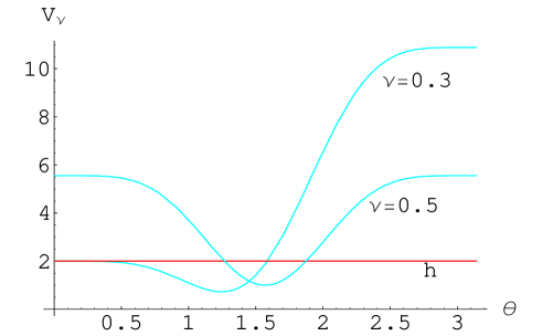
Fig. 1: $V_{\nu}(\theta)$ for $\nu=0.5$ and $0.3$. The horizontal line shows a sample line of $V_{\nu}(\theta_{0})={R^{4}h^{2}\over r_{0}^{4}+q}=2.0$. The crossing points between this line and the curves of $V_{\nu}$ correspond to $\theta_{0}$ and $\theta_{1}$.

Approximate solution:

We firstly show how the region of $\theta$ in the baryonium solutions is restriced by using $h$. From Eq. (65), we find

$${p_{\theta}^{2}\over r^{2}}+p_{r}^{2}=\left({R\over r}\right)^{4}\left({r^{4}+q\over R^{4}}V_{\nu}-h^{2}\right)\geq 0\,,$$ (11)

then it leads to

$${r^{4}+q\over R^{4}}V_{\nu}\geq h^{2}~{}.$$ (12)

For prototypical small energy solution, $r$ takes its minimum $r\simeq r_{0}$ at the mid point $x=0$. Expressing as $\theta|_{x=0}=\theta_{0}$ at this mid point, the value of $\theta_{0}$ is given by (12) as the solution of the following equation,

$${r_{0}^{4}+q\over R^{4}}V_{\nu}(\theta_{0})=h^{2}~{}.$$ (13)

This gives two solutions, $\theta_{0}$ and $\theta_{1}$ with $\theta_{0}>\theta_{1}$, as shown in the Fig. 1. Then we find that the solutions are restricted to the region $0\leq\theta\leq\theta_{1}$ or $\theta_{0}\leq\theta\leq\pi$, and they are identified with two different baryoniums.

At the mid point, $x=0$, $\theta=\theta_{0}$ and $r=r_{0}$, which are related as

$$r_{0}=\left({R^{4}h^{2}\over V_{\nu}(\theta_{0})}-q\right)^{1/4}\,.$$ (14)

Near this point, we can assume $\dot{r}\sim 0$ and $r\sim r_{0}$, and we obtain from (11)

$$\dot{\theta}=\pm{r_{0}\over R^{4}h}\sqrt{r_{0}^{4}+q}\sqrt{V_{\nu}(\theta)-V_{\nu}(\theta_{0})}$$ (15)

then it is solved as

$$x(\theta)=\pm\int_{\theta_{0}}^{\theta}d\theta~{}{R^{4}h\over r_{0}\sqrt{r_{0}^{4}+q}\sqrt{V_{\nu}(\theta)-V_{\nu}(\theta_{0})}}$$ (16)

This solution is symmetric with respect to $x=0$ axis in $x$-$\theta$ plane. The important point of this approximate solution is that the solution runs from $x=0$ to two opposite directions, however they are going to the same pole on $S^{5}$ but with different values of $x$. These two parts are considered as D5 brane and anti-D5 brane, and they can be connected at $x=0$ by a continuous flow of the $U(1)$ flux in the D5 brane. The similar behavior has been seen in other D brane and anti-D brane bound states [28, 29, 30]. We regarded this as the baryonium since the fluxes at the two end points of this configuration have the same magnitude and opposite directions.

Numerical solution

In the next, in order to see the behavior of this solution far from $\theta_{0}$, we must solve the exact form of equations as shown in [32]. An explicit example of the baryonium solution for $\nu=0.3$ is shown in the Fig. 2. This solution gives a minimum of $U$ and there is no tachyonic mode around this configuration. So this configuration is stable as shown below.

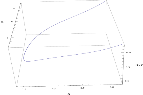
Fig. 2: A 3D representation of $D5/\overline{D5}$ solution for $R=1$, $q=0.3$, $\nu=0.3$ at $h=-.67$ and $\theta_{0}=1.42$, where $U$ takes its minimum and tachyon free.

3 Stability of the baryonium vertex

Here we study the stability of the baryonium solution obtained above. Previously, we have considered this problem from the energy density $U$ of the baryonium configurations to find its minimum as a stable solution. And we have found a minimum for $\nu=0.5$ as such an example. It has been shown through the contour graph in the $h-L$ plane, where $L$ is defined as

$$L\equiv|x_{+}(\pi)-x_{-}(\pi)|\,.$$ (17)

The baryonium solutions are considered as the bound states of D5 brane and anti-D5 brane. Then they should be separated by a definite distance to evade tachyon modes on the D5 branes. The distance between these branes is characterized by $L$, and the $U_{min}$ is found in the region of $L^{2}/R^{4}>{1\over 2\pi\alpha^{\prime}}$. This implies that the tachyonic mode of strings connecting these branes becomes massive since the mass square of this string is given as $L^{2}/R^{4}-1/(2\pi\alpha^{\prime})$ [31]. However, we must notice near the mid point of the baryonium configuration where the two branes are overlapping, then we might expect to find tachyons at this point. Here, we study this problem through the fluctuation mode around whole region of the classical configurations.

3.1 Fluctuations

In order to consider the fluctuations, we back to the action of D5 brane (4), and expand it with respect to the fluctuations, $\delta r(t,\theta)=r-\bar{r},\delta x(t,\theta)=x-\bar{x}$ and $\delta A_{t}(\theta,t)={A}_{t}-\bar{A}_{t}$, up to their quadratic terms. Here $\bar{r}$, $\bar{A}_{t}(\theta)$ and $\bar{x}$ are the solutions of the equations of motion. As for the $\delta A_{t}$, we retain it although it is not dynamical due to the lack of the kinetic term. The quadratic part of (4) for these fluctuations is given as

$$L_{(2)}=-\sin^{4}\theta~{}\left(\tilde{L}_{(2)}^{x,r}+\tilde{L}_{(2)}^{A_{t}}\right)\,,$$ (18)

where

$$\tilde{L}_{(2)}^{x,r} = A_{(2)}{\delta r}^{2}+{B_{(0)}\over 2}\left[{\delta r^{\prime}}^{2}+\left({r\over R}\right)^{4}{\delta x^{\prime}}^{2}-\left(r^{2}+{r^{\prime}}^{2}\right){\delta\dot{x}}^{2}-\left({R^{4}\over r^{2}}+{x^{\prime}}^{2}\right){\delta\dot{r}}^{2}+2x^{\prime}r^{\prime}{\delta\dot{x}}{\delta\dot{r}}\right]$$ (19)

$$+\partial_{r}\left(B_{(0)}\right)r^{\prime}{\delta r^{\prime}}{\delta r}+\partial_{r}\left({r^{4}\over R^{4}}B_{(0)}\right)x^{\prime}{\delta x^{\prime}}{\delta r}\,$$

$$-{B_{(0)}\over 2\tilde{G}_{(0)}}\left({r^{\prime}}^{2}{\delta r^{\prime}}^{2}+\left({r\over R}\right)^{8}{x^{\prime}}^{2}{\delta x^{\prime}}^{2}+2\left({r\over R}\right)^{4}r^{\prime}x^{\prime}{\delta r^{\prime}}{\delta x^{\prime}}\,,\right)$$

$$\tilde{L}_{(2)}^{A_{t}} = -\partial_{r}\left(e^{-\Phi}B_{(0)}\right)A_{t}^{\prime}{\delta A_{t}^{\prime}}{\delta r}-{e^{-\Phi}B_{(0)}\over 2}{V_{\nu}\over\sin^{8}\theta}{\delta A_{t}^{\prime}}^{2}+{e^{-\Phi}B_{(0)}\over\tilde{G}_{(0)}}A_{t}^{\prime}\left(r^{\prime}{\delta r^{\prime}}+\left({r\over R}\right)^{4}x^{\prime}{\delta x^{\prime}}\right){\delta A_{t}^{\prime}}\,$$

where $r^{\prime}=\partial_{\theta}r(\theta)$, $x^{\prime}=\partial_{\theta}x(\theta)$, $\dot{\delta r}=\partial_{t}\delta r$ and $\dot{x}=\partial_{t}\delta x$.

$$\tilde{G}_{(0)}=\left(r^{2}+(r^{\prime})^{2}+{r^{4}\over R^{4}}(x^{\prime})^{2}\right){\sin^{8}\theta\over V_{\nu}}\,.$$ (21)

$$B_{(0)}=e^{\Phi/2}/\sqrt{\tilde{G}_{(0)}}\,,\quad A_{(2)}={1\over 2}\partial_{r}^{2}\left(e^{\Phi/2}\sqrt{\tilde{G}_{(0)}}\right)\,,\quad e^{\Phi}=1+{q\over r^{4}}\,.$$ (22)

We notice here as mentioned above that $\delta A_{t}$ is not a dynamical fluctuation since there is no time derivative term for it. It can be regarded as a kind of an auxiliary field, then we integrate it out from $L_{(2)}$. It is performed by rewriting $\tilde{L}_{(2)}^{A_{t}}$ as follows,

$$\tilde{L}_{(2)}^{A_{t}}=-C_{(2)}\left(\delta A_{t}^{\prime}-\sqrt{{\tilde{L}_{(2)}^{A_{t}~{}\rm{ind}}/C_{(2)}}}\right)^{2}+\tilde{L}_{(2)}^{A_{t}~{}\rm{ind}}\,,\quad C_{(2)}={e^{-\Phi}B_{(0)}\over 2}{V_{\nu}\over\sin^{8}\theta}\,,$$ (23)

where

$$\tilde{L}_{(2)}^{A_{t}~{}\rm{ind}} = {1\over 2}{e^{2\Phi}D^{2}\over V_{\nu}}{\tilde{G}_{(0)}\over B_{(0)}}\left(-\partial_{r}\left(e^{-\Phi}B_{(0)}\right){\delta r}+{e^{-\Phi}B_{(0)}\over\tilde{G}_{(0)}}\left(r^{\prime}{\delta r^{\prime}}+\left({r\over R}\right)^{4}x^{\prime}{\delta x^{\prime}}\right)\right)^{2}\,$$

In order to remove $\delta A_{t}$, we replace $\tilde{L}_{(2)}^{A_{t}}$ by $\tilde{L}_{(2)}^{A_{t}~{}\rm{ind}}$ in (18), then we can restrict to two fluctuations $\delta x$ and $\delta r$ to see the frequency of these fluctuations, which have their time derivatives.

The modified quadratic term is obtained as

$$\tilde{L}_{(2)}\equiv\tilde{L}_{(2)}^{x,r}+\tilde{L}_{(2)}^{A_{t}~{}\rm{ind}}$$ (25)

and

$$\tilde{L}_{(2)} = \tilde{A}_{(2)}{\delta r}^{2}+{B_{(0)}\over 2}\left[\left({R^{4}\over r^{2}}+{x^{\prime}}^{2}\right)\left(-{\delta\dot{r}}^{2}+\left({r\over R}\right)^{4}{1\over Q_{(0)}}{\delta r^{\prime}}^{2}\right)+2x^{\prime}r^{\prime}{\delta\dot{x}}{\delta\dot{r}}\right.$$ (26)

$$\left.+\left(r^{2}+{r^{\prime}}^{2}\right)\left(-{\delta\dot{x}}^{2}+\left({r\over R}\right)^{4}{1\over Q_{(0)}}{\delta x^{\prime}}^{2}\right)-\left({r\over R}\right)^{4}{1\over Q_{(0)}}2x^{\prime}r^{\prime}{\delta{x^{\prime}}}{\delta{r^{\prime}}}\right]$$

$$+Q_{(1)}r^{\prime}{\delta r^{\prime}}{\delta r}+Q_{(2)}x^{\prime}{\delta x^{\prime}}{\delta r}\,$$

where

$$\tilde{A}_{(2)}={A}_{(2)}+{1\over 2}{e^{2\Phi}\tilde{G}_{(0)}\over B_{(0)}}{D^{2}\over V_{\nu}}\left(\partial_{r}\left(e^{-\Phi}B_{(0)}\right)\right)^{2}\,,\quad Q_{(0)}=r^{2}+{r^{\prime}}^{2}+{x^{\prime}}^{2}\left({r\over R}\right)^{4}$$ (27)

$$Q_{(1)}=\left(\partial_{r}\left(B_{(0)}\right)-{D^{2}\over V_{\nu}}e^{\Phi}\partial_{r}\left(e^{-\Phi}B_{(0)}\right)\right)\,,\quad Q_{(2)}=\left(\partial_{r}\left({r^{4}B_{(0)}\over R^{4}}\right)-{r^{4}D^{2}\over R^{4}V_{\nu}}e^{\Phi}\partial_{r}\left(e^{-\Phi}B_{(0)}\right)\right)\,,$$ (28)

Then we can estimate the eigenvalues of the frequency of fluctuation by imposing an appropriate boundary conditions for each eigenfunctions for these fluctuations. These eigen functions are obtained as a solution of

$$M_{ij}\vec{\delta f_{j}}=\left(\begin{array}[]{cc}M_{rr}&M_{rx}\\ M_{xr}&M_{xx}\end{array}\right)\left(\begin{array}[]{c}\delta r\\ \delta x\end{array}\right)=0\,\quad{\rm where}\quad\vec{\delta f_{j}}=(\delta r,\delta x)$$ (29)

where

$$M_{rr} = {1\over 2}\left({R^{4}\over r^{2}}+{x^{\prime}}^{2}\right)B_{(0)}\partial_{t}^{2}+\tilde{A}_{(2)}-{1\over\sin^{4}\theta}\partial_{\theta}\left({r^{4}\sin^{4}\theta\over 2R^{4}}{B_{(0)}\over Q_{(0)}}\left({R^{4}\over r^{2}}+{x^{\prime}}^{2}\right)\partial_{\theta}\right)$$ (30)

$$+Q_{(1)}r^{\prime}\partial_{\theta}\,,$$

$$M_{xx} = {r^{2}+{r^{\prime}}^{2}\over 2}B_{(0)}\partial_{t}^{2}-{1\over\sin^{4}\theta}\partial_{\theta}\left({r^{4}\sin^{4}\theta\over 2R^{4}}{B_{(0)}\over Q_{(0)}}\left[r^{2}+{r^{\prime}}^{2}\right]\partial_{\theta}\right)\,,$$ (31)

$$M_{rx} = {1\over 2}\left\{Q_{(2)}x^{\prime}\partial_{\theta}+{1\over\sin^{4}\theta}\partial_{\theta}\left({r^{4}\sin^{4}\theta\over R^{4}{Q}_{(0)}}B_{(0)}r^{\prime}x^{\prime}\partial_{\theta}\right)-r^{\prime}x^{\prime}B_{(0)}\partial_{t}^{2}\right\}\,,$$ (32)

$$M_{xr} = {1\over 2}\left\{-{\bf{1\over\sin^{4}\theta}\partial_{\theta}\sin^{4}\theta}Q_{(2)}x^{\prime}+{1\over\sin^{4}\theta}\partial_{\theta}\left({r^{4}\sin^{4}\theta\over R^{4}{Q}_{(0)}}B_{(0)}r^{\prime}x^{\prime}\partial_{\theta}\right)\right.\,,$$ (33)

$$\left.-r^{\prime}x^{\prime}B_{(0)}\partial_{t}^{2}\right\}\,,$$

In the followings, we estimate the eigen-frequencies of the fluctuations in order to see whether the solution is stable or not.

3.2 Estimation of eigen-frequencies

By assuming the following form for the fluctuations,

$$\delta r(t,\theta)=e^{i\omega_{r}t}\phi_{r}(\theta),\quad\delta x(t,\theta)=e^{i\omega_{x}t}\phi_{x}(\theta)\,,$$ (34)

we estimate the value of frequency $\omega_{r,x}$ by solving the equations given in (29) for $\theta_{0}\leq\theta\leq\pi$. Since we are intersted in the lowest eigenvalues of $\omega_{r,x}$ to see the stability of our solution. Such fluctuations are belonging to the no-node wavefunctions for $\phi_{r,x}(\theta)$. Then the equations are solved under the condition, $\phi_{r,x}(\theta_{0})=$ const. and

$$\phi_{r,x}(\pi)=0$$ (35)

or

$$\partial_{\theta}\phi_{r,x}(\pi)=0$$ (36)

for Diriclet or Neumann condition at the boundary $\theta=\pi$ respectively. The constant values at $\theta_{0}$ are determined by the normalization condition of the wave functions $\phi_{r,x}(\theta)$.

We calculated the eigenvalues for the classical configurations, which provide the minimum value of $U$ for each $\nu$, since such configurations would be stable and positive $\omega^{2}s$ are expected.

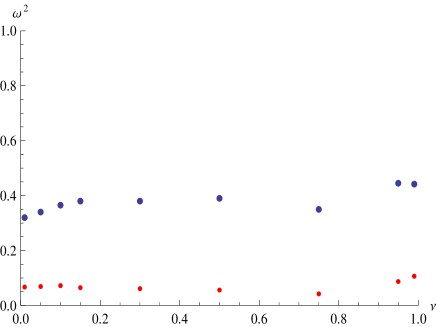
Fig. 3: The lowest for Diriclet boundary condition. The upper (lower) points show $\omega^{2}_{r}$ ($\omega^{2}_{x}$).

In the Fig. 3, we show the lowest eigenvalues for the Diriclet condition for various $\nu$. For all cases, we can see the baryonium configurations are stable against the fluctuations.

As for the Neumann condition, the lowest mode of $\delta x$ is the zero mode ($\omega_{x}=0$) with $\phi_{x}(\theta)=$ const., so we show the lowest eigenvalues of $\omega^{2}_{r}$ in the Fig. 4.

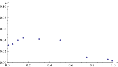
Fig. 4: The lowest $\omega^{2}_{r}$ for Neumann boundary condition.

Again, we find positive $\omega^{2}_{r}$ for any $\nu$ which implies the stability of our solutions for any $\nu$.

We notice here the following points.

(i) Firstly, the lowest eigenvalues are obtained for the zero-node wave- functions of each fluctuations, and the values of $\omega^{2}$ become large with increasing node number of the wave-functions as expected. They are abbreviated here.

(ii) In the second, we show above the eigenvalues at $U=U_{min}$, however, we could find positive eigenvalues at other values of $U$. In this sense, all the classical solutions obtained here are stable against small fluctuations around those configurations.

(iii) The next point to be noticed is that the above analysis is given for $0<\nu<1$, and the point $\nu=0$ and 1 should be excluded since the configurations in these limit of $\nu$ are not the baryonium state.

3.3 Expected configuration for $N_{c}=3$

The baryoniums are composed of the vertex, n quarks and n anti-quarks. This combination of quarks is denoted as $(n,n)$, As a practical matter, we consider here the case of $N_{c}=3$, then we find three baryonium configurations of $(3,3)$, $(2,2)$ and $(1,1)$ quarks. The one of $(2,2)$ and $(1,1)$ are shown in (a) and in (b) of the Fig. 5 respectively. They will give a good guide for baryonium hunting in the future.

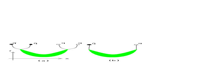
Fig. 5: Expected two baryonium configurations for $N_{c}=3$ are shown.

4 Stability of $D8/\overline{D8}$ and $D6/\overline{D6}$ as flavor branes

In the case of type IIA string theory, a holographic gauge theory is considered in the D4 brane stacked background,

$$ds^{2}_{10}=\left(\frac{U}{R}\right)^{3/2}\left(\eta_{\mu\nu}dx^{\mu}dx^{\nu}+f(U)d\tau^{2}\right)+\left(\frac{R}{U}\right)^{3/2}\left({dU^{2}\over f(U)}+U^{2}d\Omega_{4}^{2}\right)\ ,$$ (37)

where

$$f(U)=1-\left({U_{KK}\over U}\right)^{3}\,,$$ (38)

and $U_{KK}$ is related to the compact size of $S^{1}$ in the D4 world volume. Then the flavor degrees of freedom has been introduced by embedding $D8/\overline{D8}$ [30] and $D6/\overline{D6}$ [28] probe branes.

In these cases, the fundamental strings are not dissolved in the bound state branes. So the fluctuations are not affected by them as in the baryonium configurations. Our purpose to study these cases is to see the stability of those configurations agaist the fluctuations by using our method given above.

While, for a special case in [30], the stability of the configuration has been shown as mentioned below, we can show their stability for more general configurations by our method. In [28], the proof of the stability of $D6/\overline{D6}$ is abbreviated, but its stability is assured in the followings.

4.1 $D8/\overline{D8}$ branes

For the case of $D8/\overline{D8}$ probe, they are embedded with the following induced metric,

$$ds^{2}_{9}=\left(\frac{U}{R}\right)^{3/2}\eta_{\mu\nu}dx^{\mu}dx^{\nu}+\left(\left(\frac{U}{R}\right)^{3/2}f(U)\left({d\tau\over dU}\right)^{2}+\left(\frac{R}{U}\right)^{3/2}{1\over f(U)}\right)dU^{2}+\left(\frac{R}{U}\right)^{3/2}U^{2}d\Omega_{4}^{2}\ .$$ (39)

The embedded configuration of the probe brane is obtained from the D8 brane action,

$$S_{D8}\propto\int d^{4}xdUU^{4}(U/R)^{3/4}\sqrt{f(U)(\tau^{\prime})^{2}+\left(\frac{R}{U}\right)^{3}{1\over f(U)}}\,,$$ (40)

where $\tau^{\prime}=d\tau/dU$. The equation of motion for $\tau(U)$ is obtained as

$$U^{4}(U/R)^{3/4}f^{1/2}{\tau^{\prime}\over\sqrt{(\tau^{\prime})^{2}+\left(\frac{R}{U}\right)^{3}{1\over f^{2}(U)}}}=c_{0}\,,$$ (41)

where $c_{0}$ denotes an integral constant, which is taken here as

$$c_{0}=U_{0}^{4}f^{1/2}(U_{0})(U_{0}/R)^{3/4}\,.$$ (42)

Here $U_{0}(\geq U_{KK})$ denotes the minimum value of $U$ for the solution. Then the solution is given as

$$\tau(U)=\pm c_{0}\int_{U_{0}}^{U}dU\left(\frac{R}{U}\right)^{3/2}{1\over f(U)}{1\over\sqrt{U^{8}f(U)-c_{0}^{2}}}\,.$$ (43)

As in the case of the baryonium (see Eq.(16)), also this solution can be interpreted as the bound state of D8 and anti-D8 branes which are connected at $U=U_{0}$. Then we are able to study the stability of this configuration as above by checking the existence of the tachyon on the brane. The procedure is parallel to the case of the baryonium. By setting the fluctuation as $\delta\tau=\tau-\bar{\tau}$, where $\bar{\tau}$ denotes the classical solution given by Eq.(43), the D8 action is expanded by $\delta\tau$ as,

$$S_{D8}\propto\int d^{4}xdUU^{4}(U/R)^{3/4}\sqrt{f(U)G_{\tau}}\left\{1+{(R/U)^{3}\over 2G_{\tau}^{2}f^{2}(U)}(\delta\tau^{\prime})^{2}+\right.\,$$

$$\left.{(R/U)^{3}\over 2G_{\tau}f(U)}\eta^{\mu\nu}\partial_{\mu}\delta\tau\partial_{\nu}\delta\tau+\cdots\right\}\,,$$ (44)

where

$$G_{\tau}=\tau^{\prime 2}+(R/U)^{3}/f^{2}(U)\,.$$ (45)

While, at this stage, we can see that there is no tachyon for any $U_{0}$ from this form, we proceed the above procedure. By setting as $\delta\tau=f_{\tau}(x^{\mu})\phi_{\tau}(U)$, the eigenmass equation of $\delta\tau$ is obtained as follows

$$\left\{\partial_{U}\left(U^{4}\sqrt{f(U)G_{\tau}}{(R/U)^{9/4}\over G_{\tau}^{2}f^{2}(U)}\partial_{U}\right)+U^{4}\sqrt{f(U)G_{\tau}}{(R/U)^{9/4}\over G_{\tau}f(U)}m_{\tau}^{2}\right\}\phi_{\tau}(U)=0\,,$$ (46)

where $m_{\tau}^{2}$ is defined as

$$\eta^{\mu\nu}\partial_{\mu}\partial_{\nu}f_{\tau}(x^{\mu})=m_{\tau}^{2}f_{\tau}(x^{\mu})\,.$$ (47)

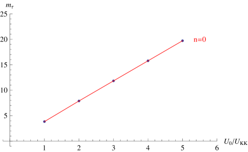
Fig. 6: The lowest value of $m_{\tau}$ versus $U_{0}/U_{KK}$ for $D8$-$\bar{D8}$. The values are for zero node wave-functions, $n=0$.

As in the previous section, we can investigate numerically the eigen mass $m_{\tau}^{2}$ of the fluctuation $\phi_{\tau}$ thorugh (46). In this case, however, the boundary condition of $\phi_{\tau}$ is taken as

$$\lim_{U\to\infty}\phi_{\tau}(U)\propto U^{-\gamma}\,,\quad\gamma>{17\over 8}$$ (48)

in order to have a normalizable wave function. This is assured from the Eq.(46), Under this condition, we find positive value as the lowest mass eigenvalue $m_{\tau}^{2}$ for any $U_{0}$. The results are shown in the Fig. 6. So we could show the stability of this brane anti-brane bound-state also. We should notice that $m_{\tau}$ increases linearly with $U_{0}/U_{KK}$ as seen from Fig.6.

Finally we notice that the stability of this configuration has been studied for the case $U_{0}=U_{KK}$ [30]. However, here, we could show its stability for any value of $U_{0}$, $U_{0}>U_{KK}$. The reason why this bound state is stable for any $U_{0}$, where D8 and anti-D8 branes are connected, is that there is no $U(1)$ flux in the brane in this case. This phenomenon seems to be universal for any bound state of D and anti-D branes.

4.2 $D4/D6$-$\bar{D6}$ branes

Instead of (37), the D4 background solution is given in [28] as follows

$$ds^{2}_{10}=\left(\frac{U}{R}\right)^{3/2}\left(\eta_{\mu\nu}dx^{\mu}dx^{\nu}+f(U)d\tau^{2}\right)+K(\rho)\left(d\lambda^{2}+\lambda^{2}d\Omega_{2}+dr^{2}+r^{2}d\phi^{2}\right)\ .$$ (49)

$$U(\rho)=\left(\rho^{3/2}+{U_{KK}^{3}\over 4\rho^{3/2}}\right)^{2/3}\,,$$ (50)

where $\rho^{2}=\lambda^{2}+r^{2}$ and

$$e^{\Phi}=g_{s}\left(\frac{U}{R}\right)^{3/4}\,,\quad f(U)=1-\left({U_{KK}\over U}\right)^{3}\,,\quad K(\rho)={R^{3/2}U^{1/2}\over\rho^{2}}\,.$$ (51)

The D6 is embedded in the following metric,

$$ds^{2}_{7}=\left(\frac{U}{R}\right)^{3/2}\eta_{\mu\nu}dx^{\mu}dx^{\nu}+R^{3/2}U^{1/2}d\Omega_{2}^{2}+\left[\left(\frac{U}{R}\right)^{3/2}f(U){\tau^{\prime}}^{2}+{1\over\left(\frac{U}{R}\right)^{3/2}f(U)}\right]dU^{2}\ .$$ (52)

Here we supposed that the profile is determined by $\tau(U)$. Then the DBI action of D6 brane is given by

$$L_{D6}=T_{D6}R^{3/2}~{}\left({U\over R}\right)^{17/4}\sqrt{f(U)G_{\tau}}\,.$$ (53)

where $G_{\tau}$ is given in Eq.(45) above. Solving the equation of motion derived from $L_{D6}$, we obtain $D4/D6$-$\bar{D6}$ embedded solution $\tau(U)$ in the background (49) as in the $D8$ case. The equation and its solution are given as follows,

$$(U/R)^{17/4}f^{1/2}{\tau^{\prime}\over\sqrt{G_{\tau}}}=d_{0}\,,$$ (54)

where the integral constant $d_{0}$ is given as

$$d_{0}=f^{1/2}(U_{0})(U_{0}/R)^{17/4}\,.$$ (55)

Here $U_{0}$ is the minimum value of $U$ and $\tau^{\prime}(U_{0})=\infty$, and the solution is given as

$$\tau(U)=\pm\int_{U_{0}}^{U}dU\left(\frac{R}{U}\right)^{3/2}{1\over f(U)}{1\over\sqrt{(U/R)^{17/4}f(U)/d_{0}^{2}-1}}\,.$$ (56)

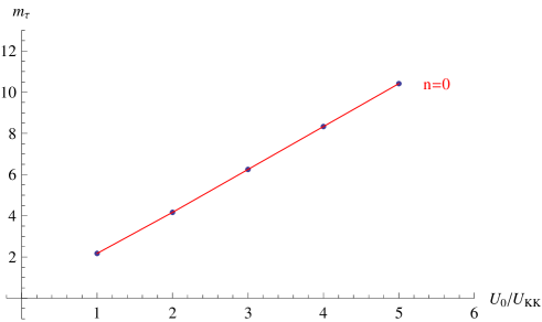
Fig. 7: The lowest value of $m_{\tau}$ versus $U_{0}/U_{KK}$ for $D6$-$\bar{D6}$. The values are for zero node wave-functions, $n=0$.

As for the fluctuation of $\tau$, we can see its quadratic term by expanding (53) with respect to $\delta\tau(=\tau-\tau_{\rm cl})$ as follows,

$$S_{D6}\propto\int d^{4}xdU(U/R)^{17/4}\sqrt{f(U)G_{\tau}}\left\{1+{(R/U)^{3}\over 2G_{\tau}^{2}f^{2}(U)}(\delta\tau^{\prime})^{2}+\right.\,$$

$$\left.{(R/U)^{3}\over 2G_{\tau}f(U)}\eta^{\mu\nu}\partial_{\mu}\delta\tau\partial_{\nu}\delta\tau+\cdots\right\}\,,$$ (57)

By setting as $\delta\tau=f_{\tau}(x^{\mu})\varphi_{\tau}(U)$, the eigenmass equation of $\varphi_{\tau}(U)$ is obtained as follows

$$\left\{\partial_{U}\left(\sqrt{f(U)G_{\tau}}{(U/R)^{5/4}\over G_{\tau}^{2}f^{2}(U)}\partial_{U}\right)+\sqrt{f(U)G_{\tau}}{(U/R)^{5/4}\over G_{\tau}f(U)}m_{\tau}^{2}\right\}\varphi_{\tau}(U)=0\,,$$ (58)

where the mass eigen-value $m_{\tau}^{2}$ is defined as above, $\eta^{\mu\nu}\partial_{\mu}\partial_{\nu}f_{\tau}(x^{\mu})=m_{\tau}^{2}f_{\tau}(x^{\mu})\,$ . The linear term of $\delta\tau$ disappears due to the field equation of $\tau$.

In solving (58), we must impose the boundary condition for $\varphi$ from the normalizability as

$$\lim_{U\to\infty}\varphi_{\tau}(U)\propto U^{-\gamma_{1}}\,,\quad\gamma_{1}>{7\over 8}\,.$$ (59)

Under this condition, we have find positive mass eigen-value $m_{\tau}^{2}$ as in the case of $D8$ branes. The results are shown in the Fig.7. In this case also, $m_{\tau}$ increases linearly with $U_{0}/U_{KK}$ as seen in the case of $D8$ branes. In any case, the $D6/\bar{D6}$ state is also stable against the fluctuation of $\tau(U)$.

5 Summary

We have examined the stability of D brane anti-D brane bound state embedded as a probe in some 10D supergravity background. We have restricted our attention to some special configurations, the baryonium state in type IIB theory and flavor branes in type IIA theory.

The vertex of the baryonium has been obtained as a bound state of D5 and anti-D5 brane in type IIB theory in terms of the D5 brane action, which wrapped on $S^{5}$ in the 10D AdS${}_{5}\times S^{5}$ and gives baryon vertex at the same time. The configuration of the baryonium is determined by the main two parameters, the gauge condensate $q$, which would determine the enrgy scale, and the flux number $(1-\nu)N_{c}$ (or $\nu N_{c}$), which is proportional to the quark number in the baryonium.

Previously, we could find an appropriate solutions of the baryonium which gives a minimum of the classical action for any value of $\nu$ and $q$. In order to confirm the stability of this configuration furthermore, this time, we have studied the time-frequency $\omega$ of the fluctuations for the relevant fields living on the D5 brane to search for the unexpected tachyonic modes. The eigen value $\omega$ has been investigated numerically for the eigen functions $\phi_{r}(\theta)$ and $\phi_{x}(\theta)$ on which the Dirichlet or Neumann boundary conditions are imposed. For both bondary conditions and at any value of $\nu$, we have found non-negative $\omega^{2}$ for the configurations given at $U=U_{min}$. Surprisingly, the non-negative $\omega^{2}$ is observed even if we consider the fluctuations around any configurations of $U(>U_{min})$. In this sense, any baryonium configuration given as the classical solution would be stable agaist the fluctuations around the baryonium solutions considered here.

As in the case of the baryon, we must add quarks to the vertex to find a complete baryonium state. The method would be parallel to the case of the baryon [18], where the no force conditions are needed at each cusp to connect $(1-\nu)N_{c}$ fundamental strings. this will be done in the near future.

We have also investigated the stability of the bound-state of $D8/\overline{D8}$ and $D6/\overline{D6}$, which are introduced as the brane for the fundamental quarks in the type IIA theory. We found that these bound states are stable. This stability would be promised by the fact that there are no $U(1)$ flux dissolved in the branes in these cases.

Appendix

A: Comment on Equation of motion

And the action is rewritten by eliminating the gauge field in terms of the solution for $\tilde{F}_{t\theta}$ given by the second equation of (2.2) to obtain an energy functional of the embedding coordinate only :

$$U={N\over 3\pi^{2}\alpha^{\prime}}\int d\theta~{}e^{\Phi/2}\sqrt{r^{2}+r^{\prime 2}+(r/R)^{4}x^{\prime 2}}\,\sqrt{V_{\nu}(\theta)}~{}.$$ (60)

$$V_{\nu}(\theta)=D(\nu,\theta)^{2}+\sin^{8}\theta$$ (61)

where we used $T_{5}\Omega_{4}R^{4}=N/(3\pi^{2}\alpha^{\prime})$.

We notice that the solution for $x(\theta)$ in our baryonium configuration is given by a two valued functions for the variable $\theta$, which is restricted to (i) $\theta_{0}\leq\theta\leq\pi$ or (ii) $0\leq\theta\leq\theta_{1}$ as explained below. So it is convenient to solve the equations by changing the variable from $\theta$ to $x$ in $U$ as,

$$U={N\over 3\pi^{2}\alpha^{\prime}}\int dx~{}e^{\Phi/2}\sqrt{r^{2}\dot{\theta}^{2}+\dot{r}^{2}+(r/R)^{4}}~{}\sqrt{V_{\nu}(\theta)},$$ (62)

where dots denotes the derivative with respect to $x$. In this form, $x$ is not contained explicitly, then we can introduce an integral constant $h$ as a “Hamiltonian” for the corresponding “time variable” $x$ as follows

$$h=\dot{r}p_{r}+\dot{\theta}p_{\theta}-L\,,\quad$$ (63)

where $L=e^{\Phi/2}\sqrt{r^{2}\dot{\theta}^{2}+\dot{r}^{2}+(r/R)^{4}}~{}\sqrt{V_{\nu}(\theta)}$ ,

$$p_{r}={\partial L\over\partial\dot{r}}=\dot{r}Q\,,\quad p_{\theta}={\partial L\over\partial\dot{\theta}}=r^{2}\dot{\theta}Q\,,\quad Q=\left({R\over r}\right)^{2}\sqrt{e^{\Phi}V_{\nu}-\left({p_{\theta}^{2}\over r^{2}}+p_{r}^{2}\right)}\,.$$ (64)

Then $h$ is rewritten in terms of the momentum as

$$h=-\left({r\over R}\right)^{2}\sqrt{e^{\Phi}V_{\nu}-\left({p_{\theta}^{2}\over r^{2}}+p_{r}^{2}\right)}\,,$$ (65)

and the Hamilton equations of motion are obtained as

$$\dot{r}={p_{r}\over Q}\,,\quad\dot{\theta}={p_{\theta}\over r^{2}Q}\,,\quad\dot{p}_{r}=-{\partial h\over\partial r}\,,\quad\dot{p}_{\theta}=-{\partial h\over\partial\theta}~{}.$$ (66)

These equations are convenient to find the baryonium vertex solutions.

References

- [1] E. Witten, “Baryons and Branes in Anti de Sitter Space,” J. High Energy Phys. 07 (1998) 006, hep-th/9805112.
- [2] D. Gross and H. Ooguri, “Aspects of Large Gauge Theory Dynamics as seen by String theory,” Phys. Rev. D58 (1998) 106002, hep-th/9805129.
- [3] Y. Imamura, “Supersymmetries and BPS Configurations on Anti-de Sitter Space,” Nucl. Phys. B537 (1999) 184, hep-th/9807179.
- [4] C. G. Callan, A. Güijosa, and K. Savvidy, “Baryons and String Creation from the Fivebrane Worldvolume Action,” hep-th/9810092.
- [5] J. Gomis, A. Ramallo, J. Simon and P. Townsend, ”Supersymmetric Baryonic Branes”, JHEP 9911 (1999) 019, hep-th/9907022
- [6] C. Callan and J. Maldacena, “Brane Dynamics from the Born-Infeld Action,” Nucl. Phys. B513 (1998) 198, hep-th/9708147.
- [7] G. Gibbons, “Born-Infeld Particles and Dirichlet p-branes”, Nucl. Phys. B514 (1998) 603, hep-th/9709027.
- [8] C. G. Callan, A. Güijosa, K. G. Savvidy and O. Tafjord, “Baryons and flux tubes in confining gauge theories from brane actions,” Nucl. Phys. B 555 (1999) 183 [arXiv:hep-th/9902197].
- [9] Y. Imamura, “On string junctions in supersymmetric gauge theories,” Prog.Theor.Phys.112:1061-1086,2004, hep-th/0410138.
- [10] A. Brandhuber, N. Itzhaki, J. Sonnenschein, and S. Yankielowicz, “Baryons from Supergravity,” J. High Energy Phys. 07 (1998) 020, hep-th/9806158.
- [11] Y. Imamura, “Baryon Mass and Phase Transitions in Large Gauge Theory,” Prog.Theor.Phys.100:1263-1272,1998, hep-th/9806162.
- [12] B. Craps, J. Gomis, D. Mateos and A. Van Proeyen, JHEP 9904 (1999) 004, [hep-th/9901060].
- [13] D. Mateos and S. Ng, JHEP 0208 (2002) 005, [hep-th/0205291].
- [14] B. Janssen, Y. Lozano, D. R. Gomez, [hep-th/0606264].
- [15] J. Maldacena, “The Large Limit of Superconformal Field Theories and Supergravity,” Adv. Theor. Math. Phys. 2 (1998) 231, hep-th/9711200.
- [16] S. S. Gubser, I. R. Klebanov, and A. M. Polyakov, “Gauge Theory Correlators from Noncritical String Theory,” Phys. Lett. B428 (1998) 105, hep-th/9802109.
- [17] E. Witten, “Anti-de Sitter Space and Holography,” Adv. Theor. Math. Phys. 2 (1998) 253, hep-th/9802150.
- [18] K. Ghoroku, M. Ishihara, “Baryons with D5 Brane Vertex and -quarks states,” Phys. Rev. D 77, 086003 (2008) [arXiv:hep-th/0801.4216].
- [19] K. Ghoroku, M. Ishihara, A. Nakamura and F. Toyoda, “Multi-quark baryon and color screening at finite temperature,” Phys. Rev. D 79, 066009 (2009) [arXiv:hep-th/0806.0195].
- [20] C. Athanasion, H. Liu and K. Rajagopal, ”Velocity dependence of baryon screening in hot strongly coupled plasma”, [arXiv:hep-th/0806.0195].
- [21] O. Bergman, G. Lifschytz and M. Lippert, “Holographic Nuclear Physics” [arXive:hep-th/0708.0302].
- [22] M. Li, Y. Zhou and S. Pu, JHEP0810:010,2008, [arXive:hep-th/0805.1611].
- [23] S. Seki and J. Sonnenschein, JHEP 0901:053,2009, [arXive:hep-th/0801.1633].
- [24] P. Burikham, A. Chatrabhuti and E. Hirunsirisawat, JHEP0905:006,2009, [arXive:hep-th/0811.0243].
- [25] H. Liu and A. A. Tseytlin, Nucl. Phys. B 553 (1999) 231 [arXiv:hep-th/ 9903091].
- [26] A. Kehagias and K. Sfetsos, Phys. Lett. B 456, 22(1999) [hep-th/9903109].
- [27] K. Ghoroku and M. Yahiro, Phys. Lett. B 604, 235 (2004) [arXiv:hep-th/ 0408040].
- [28] M. Kruczenski, D. Mateos, R. C. Myers and D. J. Winters, JHEP 0405, 041 (2004) [arXiv:hep-th/0311270].
- [29] T. Sakai and J. Sonnenschein, JHEP 0309, 047 (2003) [arXiv:hep-th/0305049].
- [30] T. Sakai and S. Sugimoto, Prog. Theor. Phys. 113, 843 (2005) [arXiv:hep-th/ 0412141].
- [31] A. Sen, APCPT Winter school lecture, 1999, [arXiv:hep-th/ 9904207].
- [32] K. Ghoroku, M. Ishihara, A. Nakamura and F. Toyoda, “Baryonium in confining gauge theories”, JHEP 04, 041 (2009) [arXiv:hep-th/0809.1137].