Tropical linear maps on the plane

Abstract

AMS class.: 15A04; 15A21; 15A33; 12K99.

Keywords and phrases: linear map, tropical geometry, projective plane.

In this paper we fully describe all tropical linear maps in the tropical projective plane $\mathbb{T}\mathbb{P}^{2}$, that is, maps from the tropical plane to itself given by tropical multiplication by a real $3\times 3$ matrix $A$. The map $f_{A}$ is continuous and piecewise–linear in the classical sense. In some particular cases, the map $f_{A}$ is a parallel projection onto the set spanned by the columns of $A$. In the general case, after a change of coordinates, the map collapses at most three regions of the plane onto certain segments, called antennas, and is a parallel projection elsewhere (theorem 3).

In order to study $f_{A}$, we may assume that $A$ is normal, i.e., $I\leq A\leq 0$, up to changes of coordinates. A given matrix $A$ admits infinitely many normalizations. Our approach is to define and compute a unique normalization for $A$ (which we call lower canonical normalization) (theorem 1) and then always work with it, due both to its algebraic simplicity and its geometrical meaning.

On $\mathbb{R}^{n}$, any $n\in\mathbb{N}$, some aspects of tropical linear maps have been studied in [6]. We work in $\mathbb{T}\mathbb{P}^{2}$, adding a geometric view and doing everything explicitly. We give precise pictures.

Inspiration for this paper comes from [3, 5, 6, 8, 12, 26]. We have tried to make it self–contained. Our preparatory results present noticeable relationships between the algebraic properties of a given matrix $A$ (idempotent normal matrix, permutation matrix, etc.) and classical geometric properties of the points spanned by the columns of $A$ (classical convexity and others); see theorem 2 and corollary 1. As a by–product, we compute all the tropical square roots of normal matrices of a certain type; see corollary 3. This is, perhaps, a curious result in tropical algebra. Our final aim is, however, to give a precise description of the map $f_{A}:\mathbb{T}\mathbb{P}^{2}\to\mathbb{T}\mathbb{P}^{2}$. This is particularly easy when two tropical triangles arising from $A$ (denoted $\mathcal{T}_{A}$ and $\mathcal{T}^{A}$) fit as much as possible. Then the action of $f_{A}$ is easily described on (the closure of) each cell of the cell decomposition $\mathcal{C}^{A}$; see theorem 3.

Normal matrices play a crucial role in this paper. The tropical powers of normal matrices of size $n\in\mathbb{N}$ satisfy $A^{\odot n-1}=A^{\odot{n}}=A^{\odot n+1}=\cdots$. This statement can be traced back, at least, to [26], and appears later many times, such as [1, 2, 6, 9, 10]. In lemma 1, we give a direct proof of this fact, for $n=3$. But now the equality $A^{\odot 2}=A^{\odot 3}$ means that the columns of $A^{\odot 2}$ are three fixed points of $f_{A}$ and, in fact, any point spanned by the columns of $A^{\odot 2}$ is fixed by $f_{A}$. Among $3\times 3$ normal matrices, the idempotent ones (i.e., those satisfying $A=A^{\odot 2}$) are particularly nice: we prove that the columns of such a matrix tropically span a set which is classically compact, connected and convex (lemma 2 and corollary 1). In our terminology, it is a good tropical triangle.

1 Introduction, Notations and Background on Tropical Mathematics

Many results on finite dimensional tropical linear algebra (spectral theory, etc.) have been published over the last 40 years and more; they are summarized in [1, 10, 14], where a wide bibliography can also be found. Two recent up–to-date collections of papers are [18, 19] In this paper we will use the adjective classical as opposed to tropical. Most definitions in tropical mathematics just mimic the classical ones. However, tropical geometry is a peculiar one. Say an inhabitant of the tropical plane is disoriented. He/she takes a look at a compass and tries to spot the tropical cardinal points. There are only three: east, north and south–west! Accordingly, he/she will set the positive part of the three coordinate axes in the given directions, when doing geometry on the plane. He/she will find out that a generic tropical line in the tropical plane looks like a tripod (it has a vertex!) although some particular tropical lines look just like classical lines, see figure 1.

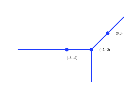
Figure 1: Tropical line with vertex at the point $(-2,-2)$.

If we happen to go down–town in a city designed by a tropical geometer, we will find out that the shape of most blocs is that of a classical hexagon, with parallel opposite sides of slopes $0,1,\infty$, see figure 2.

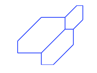
Figure 2: Downtown blocs in a tropical city.

The shortest path between two given points is made up of, at most, two classical segments with slopes $0,1,\infty$. Moreover, the distance between the given points is the sum of the integer lengths (also called lattice lengths) of these segments. For instance, the integer length between the points $(-2,-2)$ and $(0,0)$ is $2$ (not $2\sqrt{2}$!) and the integer length between the points $(-5,-2)$ and $(0,0)$ is $3+2=5$; see figure 1. This is, indeed, a sort of Manhattan distance.

So, plane tropical geometry is a funny looking piecewise–linear geometry. And, by the way, why is it called tropical? Well, the explanation appears in [13, 15], etc. and we must add that some other names have also been used (for this or akin mathematics): max–plus, dioids, path algebra, extremal algebra, idempotent mathematics, etc.

Consider the set $\mathbb{R}\cup\{-\infty\}$ endowed with tropical addition $\oplus$ and tropical multiplication $\odot$, where these operations are defined as follows:

$$a\oplus b=\max\{a,b\},\qquad a\odot b=a+b,$$

for $a,b\in\mathbb{R}\cup\{-\infty\}$. Here, $-\infty$ is the neutral element for tropical addition and $0$ is the neutral element for tropical multiplication. Notice that $a\oplus a=a$, for all $a$, i.e., tropical addition is idempotent. Notice also that $a$ has no inverse with respect to $\oplus$.

We will work with $\mathbb{R}\cup\{-\infty\}$, which will be denoted $\mathbb{T}$ and will be called the tropical semi–field. We will write $\oplus$ or $\max$, (resp. $\odot$ or $+$) at our convenience.

In classical mathematics, we have a choice in geometry: affine or projective. The tropical affine plane is $\mathbb{T}^{2}$, where addition and multiplication are defined coordinatewise. In the space $\mathbb{T}^{3}\setminus\{(-\infty,-\infty,-\infty)\}$ we define an equivalence relation $\sim$ by letting $(p_{1},p_{2},p_{3})\sim(q_{1},q_{2},q_{3})$ if there exists $\lambda\in\mathbb{R}$ such that

$$\lambda\odot(p_{1},p_{2},p_{3})=(\lambda+p_{1},\lambda+p_{2},\lambda+p_{3})=(q_{1},q_{2},q_{3}).$$

The equivalence class of $(p_{1},p_{2},p_{3})$ is denoted $[p_{1},p_{2},p_{3}]$. The tropical projective plane is the set, $\mathbb{T}\mathbb{P}^{2}$, of such equivalence classes. Notice that, at least, one of the coordinates of any point in $\mathbb{T}\mathbb{P}^{2}$ must be finite; see figure 3.

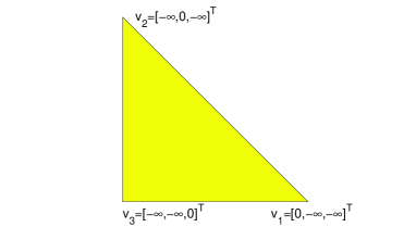
Figure 3: Tropical projective plane.

We endow the tropical plane (either affine or projective) with the topology induced by the Euclidean topology; the closure $\overline{S}$ of a set $S$ refers to this topology. In p. 8 below, we also define a tropical norm in the projective tropical plane. This norm gives rise to the Euclidean topology.

It can be easily proved that $\mathbb{T}\mathbb{P}^{2}$ is compact. $\mathbb{T}\mathbb{P}^{2}$ is a compactification of $\mathbb{T}^{2}$ (and also of $\mathbb{R}^{2}$; see p. 12). Indeed, the image of the injective map $\varphi:\mathbb{T}^{2}\to\mathbb{T}\mathbb{P}^{2}$ given by $(x,y)\mapsto[x,y,0]$ is open and dense. The boundary points are those $[x,y,-\infty]$ in $\mathbb{T}\mathbb{P}^{2}$. In fact, $\mathbb{T}\mathbb{P}^{2}$ is homeomorphic to a classical triangle in $\mathbb{R}^{2}$ (the vertices of $\mathbb{T}\mathbb{P}^{2}$ are $v_{1}=[0,-\infty,-\infty]^{T},v_{2}=[-\infty,0,-\infty]^{T}$ and $v_{3}=[-\infty,-\infty,0]^{T}$; see figure 3).

Now, for any $p=[x,y,z]$, we have $\varphi^{-1}(p)=(x-z,y-z)$, whenever $z\neq-\infty$. Taking $(x-z,y-z,0)$ as a representative of $p$ will be expressed by saying that we work in $Z=0$. In other words, to work in $Z=0$ it is just a way of passing from the projective to the affine tropical plane.

The simplest objects in the tropical plane are lines. Given a tropical linear form

$$p_{1}\odot X\oplus p_{2}\odot Y\oplus p_{3}\odot Z=\max\{p_{1}+X,p_{2}+Y,p_{3}+Z\}$$

a tropical line consists of the points $[x,y,z]\in\mathbb{T}\mathbb{P}^{2}$ where the maximum is attained, at least, twice, (this is the tropical analog of the classical vanishing point set). Denote this line by $L_{p}$, where $p=[p_{1},p_{2},p_{3}]\in\mathbb{T}\mathbb{P}^{2}$.

Most lines in the tropical plane look like tripods. Indeed, if two coefficients are equal to $-\infty$, then $L_{p}$ is a boundary component of $\mathbb{T}\mathbb{P}^{2}$. If $p_{j}=-\infty$ for just one $j$ then, in $Z=0$, $L_{p}$ is nothing but a classical slope–one line. If all $p_{j}$ are real, the $L_{p}$ is the union of three rays. The directions of these rays are west, south and north–east (just opposite to the cardinal directions of the tropical plane!) and these rays are emanating from the point $-p$, called the vertex of $L_{p}$. The latter is the generic case.

Let two points $p,q$ in the tropical plane be given. There may exist just one or infinitely many tropical lines passing through $p$ and $q$. In the latter case, just one of these lines can be described as the limit, as $\epsilon$ tends to zero, of the tropical lines going through perturbed points $p^{v_{\epsilon}},q^{v_{\epsilon}}$. Here, $p^{v_{\epsilon}}$ denotes a translation of $p$ by a length–$\epsilon$ vector $v_{\epsilon}$, see [13, 23]. We denote this limit line by $pq$ and call it the tropical stable join of $p,q$.

Now, given two tropical lines $L_{p},L_{q}$ in the plane, the stable intersection of $L_{p},L_{q}$, denoted $L_{p}\cap_{\operatorname{st}}L_{q}$, is defined as the limit point, as $\epsilon$ tends to zero, of the intersection of perturbed lines $L_{p}^{v_{\epsilon}},L_{q}^{v_{\epsilon}}$. Here, $L_{p}^{v_{\epsilon}}$ denotes a translation of $L_{p}$ by a length–$\epsilon$ vector $v_{\epsilon}$.

There exists a duality between lines and points since

$$q\in L_{p}\iff p\in L_{q},$$

meaning that the maximum $\max\{p_{1}+q_{1},p_{2}+q_{2},p_{3}+q_{3}\}$is attained, at least, twice. This duality transforms stable join into stable intersection and conversely, i.e.,

$$L_{p}\cap_{\operatorname{st}}L_{q}=r\iff pq=L_{r},$$

for $p,q,r$ in $\mathbb{T}\mathbb{P}^{2}$.

The tropical version of Cramer’s rule (see [23]) goes as follows: the stable intersection of the lines $L_{p}$ and $L_{q}$ is the point

$$[\max\{p_{2}+q_{3},q_{2}+p_{3}\},\max\{p_{1}+q_{3},q_{1}+p_{3}\},\max\{p_{1}+q_{2},q_{1}+p_{2}\}].$$

Since the computation of this point is nothing but a tropical version of the cross–product of the triples $p$ and $q$, we will denote it by $p\otimes q$ (this is not to be mixed up with $p\odot q=p+q$). Notice that $p\otimes q=q\otimes p$. In other words, the tropical version of Cramer’s rule in the plane can be written as

$$L_{p}\cap_{\operatorname{st}}L_{q}=p\otimes q\qquad\text{and}\qquad pq=L_{p\otimes q},$$

by duality. In particular, $-(p\otimes q)$ is the vertex of the line $pq$, a crucial fact that we use again and again.

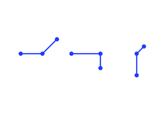
Figure 4: Tropical line segments.

Given a subset $U$ of points in $\mathbb{T}\mathbb{P}^{2}$ (resp. $\mathbb{T}^{2}$), we can consider the tropical span of $U$, denoted $\operatorname{span}(U)$, meaning the set of points $u\in\mathbb{T}\mathbb{P}^{2}$ (resp. $\mathbb{T}^{2}$) which can be written as

$$u=\lambda_{1}\odot u_{1}\oplus\cdots\oplus\lambda_{s}\odot u_{s}=\max\{\lambda_{1}+u_{1},\ldots,\lambda_{s}+u_{s}\},$$

for some $s\in\mathbb{N}$, ${u_{1},\ldots,u_{s}}\in U$, ${\lambda_{1},\ldots,\lambda_{s}}\in\mathbb{T}$, and not all $\lambda_{j}$ equal to $-\infty$ (and $\lambda_{1}\oplus\cdots\oplus\lambda_{s}=\max\{\lambda_{1},\ldots,\lambda_{s}\}=0$ when points are in $\mathbb{T}^{2}$).

The tropical co–span of $U$, denoted $\operatorname{co--span}(U)$, is the set of points $u$ which can be written as

$$u=\min\{\lambda_{1}+u_{1},\ldots,\lambda_{s}+u_{s}\},$$

for some $s\in\mathbb{N}$, ${u_{1},\ldots,u_{s}}\in U$, ${\lambda_{1},\ldots,\lambda_{s}}\in\mathbb{R}\cup\{+\infty\}$, and not all $\lambda_{j}$ equal to $+\infty$ (and $\min\{\lambda_{1},\ldots,\lambda_{s}\}=0$ when points are in $\mathbb{T}^{2}$).

Given two points $p,q\in\mathbb{T}\mathbb{P}^{2}$, we know that $-(p\otimes q)$ represents the vertex of the line $pq$. Thus $\operatorname{span}(p,q)$ is the union of the classical segments $\overline{p,-(p\otimes q)}$ and $\overline{-(p\otimes q),q}$. Dually, $\operatorname{co--span}(p,q)$ is the union of the classical segments $\overline{p,(-p)\otimes(-q)}$ and $\overline{(-p)\otimes(-q),q}$. It follows that the points $p,-(p\otimes q),q,(-p)\otimes(-q)$ are the vertices of a classical parallelogram, see figure 5.

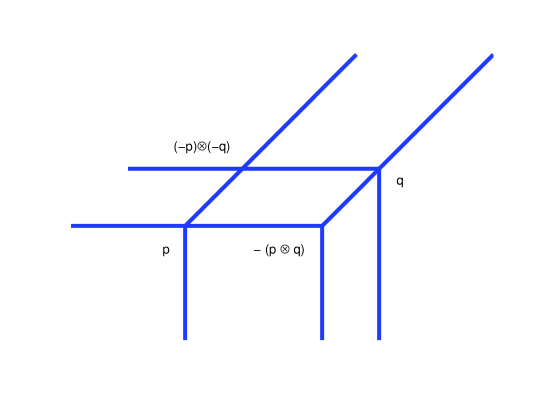
Figure 5: Span and co–span of points $p,q$.

Another sort of duality is taking place here. Indeed, we may consider $\mathbb{R}\cup\{+\infty\}$ endowed with tropical addition $\oplus^{\prime}=\min$ and the same tropical multiplication $\odot$. The relationship between these two operations is $\max\{p,q\}=-\min\{-p,-q\}$, whence

$$p\oplus q=-(-p)\oplus^{\prime}(-q),$$

for $p,q\in\mathbb{R}$. This max–min duality appears in the literature, see [4, 9, 8], etc.

Why do we care about the co–span? A tropical triangle can be determined by three points, or by three lines. First, a tropical triangle $\mathcal{T}$ is determined by three points $a,b,c$, meaning

$$\mathcal{T}=\operatorname{span}(a,b,c).$$

If the points are tropically collinear then $\mathcal{T}$ is not generic.

The sides of $\mathcal{T}$ are, by definition, the tropical lines $ab,bc$ and $ca$. The vertices of the sides of $\mathcal{T}$ (as tropical lines) are $-(a\otimes b),-(b\otimes c)$ and $-(c\otimes a)$, again by the tropical version of Cramer’s rule. The properties of the triangle $\mathcal{T}$ depend on the configuration of the six points

$$a,b,c,-(a\otimes b),-(b\otimes c),-(c\otimes a),$$ (1)

which are all different, generically.

Three tropical lines $L_{p},L_{q},L_{r}$ also determine a tropical triangle, $\mathcal{T}^{\prime}$, which is generic if the lines are not tropically concurrent. We can write

$$\mathcal{T}^{\prime}=\operatorname{co--span}(-p,-q,-r).$$

The stable intersections (by pairs) of the lines $L_{p},L_{q},L_{r}$ are called vertices of $\mathcal{T}^{\prime}$. These points should not be mixed up with the vertices $-p,-q,-r$ of the lines. By the tropical version of Cramer’s rule, the coordinates of the vertices of $\mathcal{T}^{\prime}$ are $p\otimes q,q\otimes r$ and $r\otimes p$. The properties of $\mathcal{T}^{\prime}$ depend on the configuration of the six points

$$p\otimes q,q\otimes r,r\otimes p,-p,-q,-r,$$

which are all different, in the generic case.

A tropical segment is the tropical span of two points (see fig. 4). Tropical triangles are, in general, infinite unions of tropical segments. Indeed,

$$\mathcal{T}=\operatorname{span}(a,b,c)=\bigcup_{s\in\operatorname{span}(b,c)}\operatorname{span}(a,s).$$ (2)

Therefore, tropical triangles are, in general, connected non–pure two–dimensional sets. The non–generic case arises when the points $a,b,c$ are tropically collinear (either being $a,b,c$ all different or not). In addition, it is easy to check that tropical triangles are classically compact, both in $\mathbb{T}\mathbb{P}^{2}$ and in $\mathbb{T}^{2}$.

It is not true, in general, that the stable intersection of the tropical lines $ab$ and $bc$ gives back the point $b$, and this makes tropical triangles trickier than classical triangles. For example, take $a=[3,4,6]$, $b=[-2,0,8]$ and $c=[1,1,0]$ Then $a\otimes b=[12,11,3],b\otimes c=[9,9,1]$ and $ab\cap_{\operatorname{st}}bc=[12,13,21]=[-1,0,8]\neq b$. The reader is encouraged to draw this example, in $Z=0$.

This anomalous situation for tropical triangles has been studied in [3], where the definition of good tropical triangle has been given. Three points $a,b,c$ define a good tropical triangle if, by stable join, they give rise to three tropical lines $ab,bc,ca$ which, stably intersected by pairs, yield the original points $a,b,c$, i.e.,

$$ca\cap_{\operatorname{st}}ab=a,\quad ab\cap_{\operatorname{st}}bc=b,\quad bc\cap_{\operatorname{st}}ca=c.$$

Good tropical triangles are characterized by six slack inequalities. Indeed, write the coordinates of (representatives of) $a,b,c$ as the columns of a matrix $A=(a_{ij})$ so that $c$ occupies the first column and $a$ occupies the third. Write

$$\mathcal{T}_{A}=\operatorname{span}(A).$$ (3)

Then theorem 2 in [3] tells us that $\mathcal{T}_{A}\subseteq\mathbb{T}\mathbb{P}^{2}$ is a good tropical triangle if and only if

$$a_{12}-a_{22}\leq a_{13}-a_{23}\leq a_{11}-a_{21},$$

$$a_{23}-a_{33}\leq a_{21}-a_{31}\leq a_{22}-a_{32},$$ (4)

$$a_{31}-a_{11}\leq a_{32}-a_{12}\leq a_{33}-a_{13}.$$

In order to make drawings in $Z=0$ we consider the matrix

$$A_{0}=\left[\begin{array}[]{ccc}a_{11}-a_{31}&a_{12}-a_{32}&a_{13}-a_{33}\\ a_{21}-a_{31}&a_{22}-a_{32}&a_{23}-a_{33}\\ 0&0&0\\ \end{array}\right].$$

It is easy to check that the six inequalities (4) imply the following cardinal points condition in $Z=0$: $\operatorname{col}(A_{0},1)$ represents the most eastwards point, $\operatorname{col}(A_{0},2)$ represents the most northwards one, and $\operatorname{col}(A_{0},3)$ represents the most south–westwards one, among the columns of $A_{0}$. More precisely, starting at $\operatorname{col}(A_{0},1)$, we walk $a_{22}-a_{32}-a_{21}+a_{31}\geq 0$ units northbound, then walk $a_{11}-a_{31}-a_{12}+a_{32}\geq 0$ units westbound and we reach $\operatorname{col}(A_{0},2)$. From there, we walk $a_{33}-a_{13}-a_{32}+a_{12}\geq 0$ units south–westbound, then walk $a_{22}-a_{12}-a_{23}+a_{13}\geq 0$ units southbound, to reach $\operatorname{col}(A_{0},3)$. In a similar manner we get from $\operatorname{col}(A_{0},3)$ to $\operatorname{col}(A_{0},1)$ by walking first eastbound, then north–eastbound. The distances are dictated by inequalities (4).

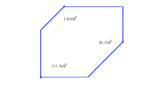
Figure 6: Good triangle determined by the matrix $A$.

In figure 6 we have the good tropical triangle determined by the matrix

$$A=A_{0}=\left[\begin{array}[]{ccc}0&-5&-7\\ -3&0&-6\\ 0&0&0\end{array}\right].$$

In simple words, in $Z=0$, good tropical triangles are nothing but classical hexagons, pentagons, quadrangles or triangles having slopes $0,1$ and $\infty$, where the inequalities (4) provide the integer length of the sides. The hexagons are obtained by chopping off two corners, in a classical rectangle of sides parallel to axis $X,Y$, see figure 7. The pentagons, quadrangles or triangles arise from one such hexagon, when one or more sides collapse to a point. In figure 8 we see a few good triangles. Here is one more way to describe good triangles: any $a\leq b$, $c\leq d$ and $e\leq f$ in $\mathbb{R}$ define the following good tropical triangle in $Z=0$:

$$\mathcal{T}=\{(x,y)\in\mathbb{R}^{2}:a\leq x\leq b,\ c\leq y\leq d,\ e\leq y-x\leq f\}.$$ (5)

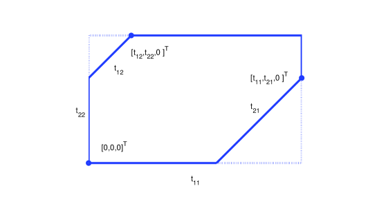
Figure 7: A good tropical triangle is a classical rectangle with two corners chopped off.

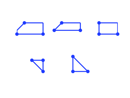
Figure 8: Some good tropical triangles.

In the classical plane $\mathbb{R}^{2}$ we have the following norm

$$\|p\|=\max\{\|p_{1}\|,\|p_{2}\|,\|p_{1}-p_{2}\|\},\qquad p\in\mathbb{R}^{2}.$$

It is easy to check that $\|p\|$ is the integer length of the tropical segment $\operatorname{span}(p,0)$, if we identify $p=(p_{1},p_{2})$ with $[p_{1},p_{2},0]$. For instance, $\|(-5,-2)\|=5$, $\|(-3,5)\|=8$. The unit ball and some radii in it are shown in figure 9. Given real points $p,q\in\mathbb{R}^{2}$ the tropical distance between $p$ and $q$ is $\|p-q\|$, by definition. It is the integer length of the tropical segment $\operatorname{span}(p,q)$. This is connected with the Hilbert projective metric appearing in [8, 12, 16] and to the range seminorm of [11].

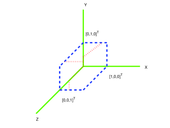
Figure 9: Axes and unit ball in the tropical the plane. Some rays are shown in dotted lines.

In $\mathbb{T}\mathbb{P}^{2}$, let $V$ be the tropical span of a finite family of points. In [8, 12, 16], a projector map (or nearest point map) $\rho:\mathbb{T}\mathbb{P}^{2}\to V$ is considered. It satisfies $\rho\circ\rho=\rho$ and $\rho|_{V}=\operatorname{id}_{V}$. For a point $p\in\mathbb{T}\mathbb{P}^{2}\setminus V$, the image $\rho(p)$ is computed as follows: fix a representative $p^{\prime}\in\mathbb{T}^{3}$ of $p$ and, for each generator $v$ of $V$, choose a representative $v^{\prime}\in\mathbb{T}^{3}$, optimal for the condition $v^{\prime}\leq p^{\prime}$ (meaning $v^{\prime}_{j}\leq p^{\prime}_{j}$, for $j=1,2,3$ and equality is attained for, at least, one $j$). Tropically add all such $v^{\prime}s$ and then, take $\rho(p)$ to be the point in $\mathbb{T}\mathbb{P}^{2}$ represented by the sum. In [8, 12, 16] it is shown that $\rho(p)\in V$ minimizes the tropical distance $\|p-q\|$, when $q$ runs through $V$. In general, there are infinitely many points $q$ in $V$ minimizing such a distance, in addition to $\rho(p)$. Indeed, consider tropical balls $B(d)$ centered at $p$ of increasing radius $d$ and take the minimum $d>0$ such that the intersection $B(d)\cap V$ is non–empty. Then $B(d)\cap V$ is the set of minimizing points.

2 Matrices, maps and pictures in $Z=0$

All arrays will have entries in $\mathbb{T}$. Arrays will be denoted by capital letters $A,B,C$, $N,P,Q$, etc. Tropical matrix addition and multiplication are defined in the usual way, but using the tropical operations $\oplus$ and $\odot$, instead of the classical ones. Any array all whose entries are zero will be denoted by 0. Given two arrays of the same size $A=(a_{ij})$, $B=(b_{ij})$, we will write $A\leq B$ if $a_{ij}\leq b_{ij}$, for all $i,j$.

We will deal with $3\times 3$ matrices. The tropical determinant of a $3\times 3$ matrix $A=(a_{ij})$ (also called tropical permanent) is defined as

$$|A|_{trop}=\max_{\sigma\in\Sigma_{3}}\{a_{1\sigma(1)}+a_{2\sigma(2)}+a_{3\sigma(3)}\},$$

where $\Sigma_{3}$ denotes the symmetric group in $3$ symbols. A matrix is tropically singular if the maximum in the tropical determinant is attained, at least, twice. Otherwise the matrix is tropically regular, or it is said to have a strong permanent. These are all standard definitions.

Given a matrix $A$, the $j$–th column (resp. row) of $A$ will be denoted $\operatorname{col}(A,j)$ (resp. $\operatorname{row}(A,j)$). The triple of diagonal entries of $A$ will be denoted $\operatorname{diag}(A)$. Moreover, if $t\in\mathbb{R}^{3}$, then $\operatorname{diag}(t)$ will denote the matrix whose diagonal is $t$, the rest of entries being equal to $-\infty$; such matrices will be called diagonal matrices. A permutation matrix is a matrix obtained from a diagonal matrix, by permuting some of its rows or permuting some of its columns. A particular case is the tropical identity matrix, $I=\operatorname{diag}(0)$. Another example is

$$P_{12}=\left[\begin{array}[]{ccc}-\infty&0&-\infty\\ 0&-\infty&-\infty\\ -\infty&-\infty&0\\ \end{array}\right].$$

Any permutation matrix $P$ has a tropical inverse $P^{\odot-1}$, meaning $P\odot P^{\odot-1}=P^{\odot-1}\odot P=I$.

From now on, points in $\mathbb{T}\mathbb{P}^{2}$ will be denoted by columns, for convenience. We often identify a $3\times 3$ matrix $A$ with the three points in $\mathbb{T}\mathbb{P}^{2}$ represented by its columns.

The reader can easily check that left–multiplication by the matrix $P_{12}$ exchanges coordinates $X$ and $Y$:

$$P_{12}\odot\left[\begin{array}[]{c}x\\ y\\ z\end{array}\right]=\left[\begin{array}[]{c}y\\ x\\ z\end{array}\right].$$

A triple $t=(t_{1},t_{2},t_{3})\in\mathbb{R}^{3}$ gives rise to a translation in $\mathbb{T}\mathbb{P}^{2}$:

$$\left[\begin{array}[]{c}X\\ Y\\ Z\end{array}\right]\mapsto\left[\begin{array}[]{c}X^{\prime}\\ Y^{\prime}\\ Z^{\prime}\end{array}\right]=\left[\begin{array}[]{c}t_{1}+X\\ t_{2}+Y\\ t_{3}+Z\end{array}\right]=\operatorname{diag}(t)\odot\left[\begin{array}[]{c}X\\ Y\\ Z\end{array}\right],$$

By a change of projective coordinates in the tropical projective plane $\mathbb{T}\mathbb{P}^{2}$ we mean left–multiplying coordinates by a permutation matrix. Therefore, a change of projective coordinates amounts to the composition of a translation and a permutation of coordinates. Notice that right–multiplying $A$ by a diagonal matrix does not change the columns of $A$ in $\mathbb{T}\mathbb{P}^{2}$; it only changes the representatives of them.

All pictures will be done in the affine tropical plane $Z=0$. In order to do so, from a given matrix $A$ we compute the matrix

$$A_{0}=A\odot\operatorname{diag}(-\operatorname{row}(A,3)).$$ (6)

From now on, suppose that $A$ is real. Our aim is to describe the map $f_{A}:\mathbb{T}\mathbb{P}^{2}\to\mathbb{T}\mathbb{P}^{2}$

$$\left[\begin{array}[]{c}x\\ y\\ z\end{array}\right]\mapsto A\odot\left[\begin{array}[]{c}x\\ y\\ z\end{array}\right]=\left[\begin{array}[]{c}\max\{a_{11}+x,a_{12}+y,a_{13}+z\}\\ \max\{a_{21}+x,a_{22}+y,a_{23}+z\}\\ \max\{a_{31}+x,a_{32}+y,a_{33}+z\}\\ \end{array}\right].$$

First, notice that proportional matrices $A$ and $\lambda\odot A$ determine the same map $f_{A}=f_{\lambda\odot A}$, any $\lambda\in\mathbb{R}$. The simplest examples of maps $f_{A}$ arise for $A=I$ (resp. $A=0$), the map being the identity (resp. constant). It is constant also for $f_{A\odot 0}$ and $f_{0\odot A}$, because all the columns of $A\odot 0$ (resp. $0\odot A$) represent the same point in $\mathbb{T}\mathbb{P}^{2}$.

The map $f_{A}$ is obviously continuous and piecewise–linear. The image $\operatorname{im}f_{A}$ is the tropical triangle spanned by $A$, meaning that it is spanned by the columns of $A$:

$$\mathcal{T}_{A}=\operatorname{im}f_{A}=\operatorname{span}(A).$$ (7)

The map $f_{A}$ is not surjective, since no finite family of points with finite coordinates span the whole $\mathbb{T}\mathbb{P}^{2}$; this is well–known (see, e.g., [25]). Moreover, if $r,s\in\mathbb{R}$ are negative and big enough, we have

$$A\odot\left[\begin{array}[]{c}0\\ r\\ s\end{array}\right]=\operatorname{col}(A,1),\ A\odot\left[\begin{array}[]{c}s\\ 0\\ r\end{array}\right]=\operatorname{col}(A,2),\ A\odot\left[\begin{array}[]{c}r\\ s\\ 0\end{array}\right]=\operatorname{col}(A,3).$$

Therefore, $f_{A}$ is locally constant on three big chunks of $\mathbb{T}\mathbb{P}^{2}$, called corners; see figure 10. In particular, $f_{A}$ is not injective.

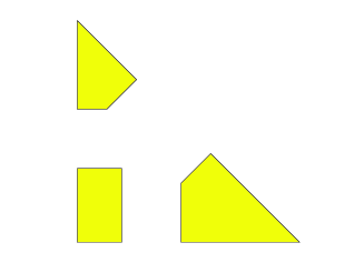
Figure 10: Corners.

Let us see how do these corners arise. First, the matrix $A$ defines three tropical lines $A_{1},A_{2},A_{3}$, because the $j$–th row of $A$ provides a tropical linear form

$$a_{j1}\odot X\oplus a_{j2}\odot Y\oplus a_{j3}\odot Z=\max\{a_{j1}+X,a_{j2}+Y,a_{j3}+Z\}.$$

The vertices of $A_{1},A_{2},A_{3}$ are (represented by) the rows of $-A$, i.e., the columns of $-A^{T}$. Thus we have another tropical triangle here, namely

$$\mathcal{T}^{A}=\operatorname{co--span}(-A^{T}).$$ (8)

The lines $A_{1},A_{2},A_{3}$ (or, rather, the matrix $A$) induce a cell decomposition on $\mathbb{R}^{2}$, denoted $\mathcal{C}^{A}_{\mathbb{R}}$ (see [12] for an isomorphic cell decomposition). The decomposition $\mathcal{C}^{A}_{\mathbb{R}}$ consists of, at most, 31 cells, and this is the generic case. Every cell $\Gamma$ is relatively open, i.e., $\Gamma$ is open inside its affine hull in $\mathbb{R}^{2}$.

In $\mathcal{C}^{A}_{\mathbb{R}}$ we have:

• ten two–dimensional cells: one bounded cell, denoted $B^{A}$, the three already mentioned corners (denoted $C^{A}_{1},C^{A}_{2},C^{A}_{3}$), six unbounded cells (parallel to some tropical coordinate axis $X,Y$ or $Z$),

• fifteen one–dimensional cells: nine unbounded cells (parallel to some coordinate axis) and six bounded cells,

• six zero–dimensional cells or points.

Notice that the union of all the bounded cells above is nothing but $\mathcal{T}^{A}$. Moreover, $\overline{B^{A}}$ is the union of some bounded cells.

For later use, bounded cells will also be called central cells; all other cells will be called peripheral cells. In figure 12 we find the 31 cells described above, and figure 11 represents the cell decomposition induced by the matrix

$$A=\left[\begin{array}[]{ccc}0&-1&-5\\ -4&0&-2\\ -1&-4&0\end{array}\right],\ (-A^{T})_{0}=\left[\begin{array}[]{ccc}-5&2&1\\ -4&-2&4\\ 0&0&0\end{array}\right].$$ (9)

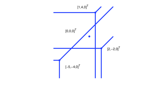
Figure 11: Cell decomposition $\mathcal{C}^{A}_{\mathbb{R}}$ induced by matrix $A$ in (9).

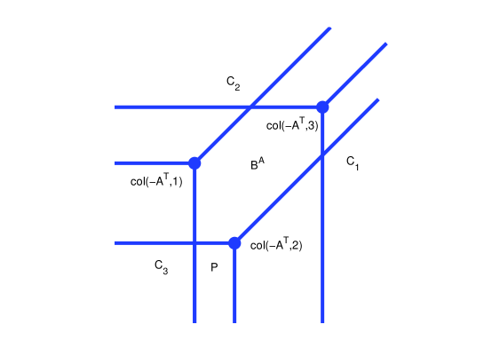
Figure 12: The 31 cells in the cell decomposition $\mathcal{C}^{A}_{\mathbb{R}}$ induced by some matrix $A$.

$\mathbb{T}\mathbb{P}^{2}$ is a compactification of $\mathbb{R}^{2}$; cf. p. 3. The set of boundary points of this compactification is

$$\partial=\mathbb{T}\mathbb{P}^{2}\setminus\mathbb{R}^{2}=\{[x,y,z]^{T}:x=-\infty\text{\ or\ }y=-\infty\text{\ or\ }z=-\infty.\}$$

Therefore, the cell decomposition $\mathcal{C}^{A}_{\mathbb{R}}$ induces a cell decomposition $\mathcal{C}^{A}$ of $\mathbb{T}\mathbb{P}^{2}$, which, in addition to all the cells in $\mathcal{C}^{A}_{\mathbb{R}}$, contains

• $k$ one–dimensional cells,

• $k$ zero–dimensional cells or points,

for some $3\leq k\leq 12$. The union of these additional cells is $\partial$. Notice that in most of our figures, we have not drawn $\partial$. Since $\mathbb{T}\mathbb{P}^{2}$ is compact, it no longer makes sense talking about unbounded cells, but we have already introduced the alternative term peripheral. Recall that $B^{A}$ is the central two–dimensional cell. For instance, $B^{A}$ is empty, if $A=0$.

The description of the map $f_{A}:\mathbb{T}\mathbb{P}^{2}\to\mathbb{T}\mathbb{P}^{2}$ is particularly easy when the tropical triangles $\mathcal{T}_{A}$ and $\mathcal{T}^{A}$ fit as much as possible: then the action of $f_{A}$ is easily described on the closure of each cell $\Gamma$ of the decomposition $\mathcal{C}^{A}$; see theorem 3.

3 Normal matrices

By definition, a matrix $A$ is normal if $\operatorname{diag}(A)=0$ and $A\leq 0$; in symbols,

$$I\leq A\leq 0$$ (10)

see [6]; in [10] a matrix $A$ such that $I\leq A$ is called increasing. For any matrix $A$ there exist permutation matrices $P,Q$ such that the product

$$N=P\odot A\odot Q$$ (11)

is normal. The matrix $N$ is called a normalization of $A$. The Hungarian method (see [6, 17, 22]) is an algorithm to obtain such $N,P,Q$. A matrix $A$ admits several normalizations. Notice that the columns of $A$ and the columns of $A\odot Q$ represent the same points in $\mathbb{T}\mathbb{P}^{2}$, given perhaps in a different order. And the columns of $N$ are a just a translation of those points.

As in classical mathematics, the product of matrices corresponds to the composition of maps:

$$f_{N}=f_{P}\circ f_{A}\circ f_{Q}.$$

Now, $f_{P}$ and $f_{Q}$ are changes of projective coordinates, so that in order to study the map $f_{A}$, we may assume that $A$ is normal, up to changes of coordinates.

A normal matrix $A$ satisfies $I\leq A\leq 0$, and therefore

$$I\leq A\leq A^{\odot 2}\leq A^{\odot 3}\leq\cdots$$ (12)

and, for any natural number $m$,

$$A^{\odot m+1}\leq A^{\odot m}\odot 0$$ (13)

since tropical multiplication by any matrix is monotonic (because max and $+$ are monotonic). And the map $f_{A^{\odot m}\odot 0}$ is constant, as explained in p. 2.

In corollary 3 we will see that the tropical powers of $A$ are simpler than $A$ (in the sense that they depend on fewer parameters), when $A$ belongs to a particular class of normal matrices. This simplification will carry over to the corresponding maps

$$\operatorname{id}=f_{I},f_{A},f_{A^{\odot 2}},f_{A^{\odot 3}},\ldots,\operatorname{const}.$$

Consider the cell decomposition $\mathcal{C}^{0}$ induced by the zero matrix on $\mathbb{T}\mathbb{P}^{2}$; it is just the cell decomposition given by the tropical line $L_{0}$. It has three two–dimensional cells (corners), which have the following description in $Z=0$:

$$C^{0}_{1}=\{0<x,y<x\},\qquad C^{0}_{2}=\{0<y,x<y\},\qquad C^{0}_{3}=\{x<0,y<0\}.$$

The geometric meaning of normality is the following: if $A$ is a $3\times 3$ normal matrix then,

$$\operatorname{col}(A_{0},j)\in\overline{C^{0}_{j}},\quad\text{for all}\quad j=1,2,3.$$ (14)

Next we define several operators on matrices and then we study the relationship among them. Of course, we are particularly interested in these operators acting on normal matrices.

For any $k\in\mathbb{N}$, the tropical $k$–th power of $A$, denoted $A^{\odot k}$, takes normal matrices to normal matrices. The transpose $A^{T}$ of a normal matrix $A$ is a normal matrix. These operators commute with each other. Warning: $(-A)^{\odot 2}\neq A^{\odot 2}$, in general. Also, $(A_{0})^{\odot 2}\neq(A^{\odot 2})_{0}$, in general.

We introduce the tropical adjoint of $A$, denoted $\widehat{A}$. By definition, $\widehat{A}=(\alpha_{ij})$, where $\alpha_{ij}$ is the tropical cofactor of $a_{ji}$. In other words,

$$\operatorname{row}(\widehat{A},j)=\operatorname{col}(A,j-1)\otimes\operatorname{col}(A,j+1),$$ (15)

for $j=1,2,3,\mod 3$. Last, we define an auxiliary matrix operator, $\breve{A}=(\beta_{ij})$, by the formulas

$$\beta_{ii}=0,\qquad\beta_{ij}=a_{ik}+a_{kj},\qquad\text{\ if \ }i\neq j\text{\ and\ }\{i,j,k\}=\{1,2,3\}.$$

Lemma 1.

If $A$ is $3\times 3$ normal, then

1. $\breve{A}$ is normal and $\widehat{A}=A\oplus\breve{A}=A^{\odot 2}$,

2. $\widehat{A}$ is normal,

3. $A^{\odot 2}=A^{\odot 3}$,

4. every point in $\mathcal{T}_{A^{\odot 2}}=\operatorname{span}(A^{\odot 2})$ is fixed by $f_{A}$,

5. zero (the neutral element for tropical multiplication) is an eigenvalue of $A$.

Proof.

A straightforward computation yields (1) and then (2) follows. Now, multiplication by $A$ is a monotonic operator; so that the equality in (1) implies $A^{\odot 3}=\max\{A^{\odot 2},A\odot\breve{A}\}$. Now, a simple computation shows that $A\odot\breve{A}=A\oplus\breve{A}$, whence $A^{\odot 3}=A^{\odot 2}$ follows. Finally, (4) follows from (3) and (5) follows from (4). ∎

Lemma 1 follows from [26], where real matrices of any size $n$ are considered. The so called Kleene star of $A$ (or strong closure of $A$) is defined as

$$A^{*}=I\oplus A\oplus A^{\odot 2}\oplus A^{\odot 3}\oplus\cdots,$$

if the limit exists, see[1, 7]. If $A$ is a $3\times 3$ normal matrix, then $A^{*}=A^{\odot 2}$, but we will not use this.

Lemma 2.

For a $3\times 3$ normal matrix $A$, the following are equivalent:

1. $\breve{A}\leq A$,

2. $A=A^{\odot 2}$, i.e., $A$ is idempotent,

3. $\mathcal{T}_{A}$ is good.

Proof.

The equivalence follows from lemma 1 and the six inequalities (4), letting $a_{jj}=0$, for $j=1,2,3$. Indeed, we obtain

$$a_{23}+a_{31}\leq a_{21},\qquad a_{32}+a_{21}\leq a_{31},$$

$$a_{13}+a_{32}\leq a_{12},\qquad a_{31}+a_{12}\leq a_{32},$$ (16)

$$a_{12}+a_{23}\leq a_{13},\qquad a_{21}+a_{13}\leq a_{23}.$$

∎

Suppose $A=(a_{ij})$ is normal and consider

$$A_{0}=\left[\begin{array}[]{ccc}-a_{31}&a_{12}-a_{32}&a_{13}\\ a_{21}-a_{31}&-a_{32}&a_{23}\\ 0&0&0\end{array}\right].$$

By a translation, we can assume that $a_{13}=a_{23}=0$, so that $\operatorname{col}(A_{0},3)=0$. Write

$$t_{11}=-a_{31},\ t_{22}=-a_{32},\ t_{21}=a_{21}-a_{31},\ t_{12}=a_{12}-a_{32},$$ (17)

so that

$$A_{0}=\left[\begin{array}[]{ccc}t_{11}&t_{12}&0\\ t_{21}&t_{22}&0\\ 0&0&0\\ \end{array}\right]$$ (18)

If, in addition, $A$ is idempotent, then

$$0\leq t_{11},t_{22},\quad 0\leq t_{21},t_{12}\leq\min\{t_{11},t_{22}\}$$ (19)

and these $t_{ij}$ provide a parameter space for good tropical triangles, up to translation; see figure 7.

The six points listed in (1) are (represented by) the columns of $A$ and of $-\widehat{A}^{T}$, according to the definition of adjoint matrix. They determine the shape of the tropical triangle $\mathcal{T}_{A}$.

Lemma 3.

If $A$ is a $3\times 3$ idempotent normal matrix, then $A^{T}=(A^{\odot 2})^{T}=\widehat{A}^{T}$. In particular, $\mathcal{T}_{A}$ is determined by the columns of $A$ and of $-A^{T}$.∎

Figure 13 illustrates the former lemma.

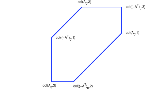
Figure 13: Tropical triangle associated to an idempotent normal matrix.

4 Canonical normalization

The geometric meaning of canonical normalization is getting pictures centered at the origin of $Z=0$. We have two equivalent ways to achieve this goal: upper and lower canonical normalization. The difference is irrelevant: just an exchange of coordinates $X$ and $Y$. Our choice will be lower canonical normalization. We have used $L$ (resp. $U$) to mean lower (resp. upper).

For each $d,d_{1},d_{2},d_{3}\in\mathbb{R}$ consider the matrix

$$L(d,d_{1},d_{2},d_{3})=\left[\begin{array}[]{ccc}0&-d-d_{2}&-2d-d_{3}\\ -2d-d_{1}&0&-d-d_{3}\\ -d-d_{1}&-2d-d_{2}&0\\ \end{array}\right]$$ (20)

Notice the symmetric role played by $d_{1}$ with respect to $X$, $d_{2}$ with respect to $Y$ and $d_{3}$ with respect to $Z$. We will use the matrices

$$L(d,d_{1},d_{2},d_{3})_{0}=\left[\begin{array}[]{ccc}d+d_{1}&d&-2d-d_{3}\\ -d&2d+d_{2}&-d-d_{3}\\ 0&0&0\\ \end{array}\right],$$ (21)

$$(-L(d,d_{1},d_{2},d_{3})^{T})_{0}=\left[\begin{array}[]{ccc}-2d-d_{3}&d+d_{1}-d_{3}&d+d_{1}\\ -d+d_{2}-d_{3}&-d-d_{3}&2d+d_{2}\\ 0&0&0\end{array}\right].$$ (22)

It is easy to check that if $d\geq 0$ and $-d\leq d_{j}$, for $j=1,2,3$ then $L(d,d_{1},d_{2},d_{3})$ is normal. If, in addition, $d_{1},d_{2},d_{3}\geq 0$, then $A$ is also idempotent. In this case, $\mathcal{T}_{A}$ reduces to a segment if and only if $d=d_{j}=d_{j+1}=0$, for some $j=1,2,3$ modulo 3, and $\mathcal{T}_{A}$ reduces to a point if and only if $d=d_{1}=d_{2}=d_{3}=0$.

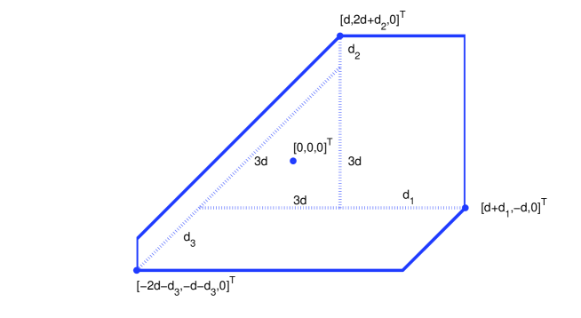
Figure 14: Tropical triangle given by the matrix $L(d,d_{1},d_{2},d_{3})$, in $Z=0$. Dotted lines are auxiliary.

In a similar fashion we can consider the matrix

$$U(d,d_{1},d_{2},d_{3})=\left[\begin{array}[]{ccc}0&-2d-d_{2}&-d-d_{3}\\ -d-d_{1}&0&-2d-d_{3}\\ -2d-d_{1}&-d-d_{2}&0\\ \end{array}\right].$$

Notice that $P_{12}U(d,d_{1},d_{2},d_{3})P_{12}=L(d,d_{2},d_{1},d_{3})$.

Lemma 4 (Lower canonical normalization for an idempotent normal matrix).

If $A$ is a $3\times 3$ idempotent normal matrix, then there exist unique $d,d_{1},d_{2},d_{3}\geq 0$ and there exist permutation matrices $P,Q$ such that $L(d,d_{1},d_{2},d_{3})=P\odot A\odot Q$.

Proof.

A translation allows us to assume that $\operatorname{col}(A_{0},3)=0$. Then

$$A_{0}=\left[\begin{array}[]{ccc}t_{11}&t_{12}&0\\ t_{21}&t_{22}&0\\ 0&0&0\end{array}\right],\qquad A=\left[\begin{array}[]{ccc}0&t_{12}-t_{22}&0\\ t_{21}-t_{11}&0&0\\ -t_{11}&-t_{22}&0\end{array}\right],$$

with $0\leq t_{11},t_{22}$ and $0\leq t_{21},t_{12}\leq\min\{t_{11},t_{22}\}$.

Assume that $t_{21}\leq t_{12}$ (see figure 15). Then we take $d=\frac{1}{3}(t_{12}-t_{21})$, $d_{1}=t_{11}-t_{12}$, $d_{2}=t_{22}-t_{12}$, $d_{3}=t_{21}$ and $Q=\operatorname{diag}(d_{3}+2d,d_{3}+d,0)$, obtaining $L(d,d_{1},d_{2},d_{3})=Q^{\odot-1}\odot A\odot Q$.

Now, assume that $t_{21}\geq t_{12}$ (see figure 16). Then we take $d=\frac{1}{3}(t_{21}-t_{12})$, $d_{2}=t_{11}-t_{21}$, $d_{1}=t_{22}-t_{21}$, $d_{3}=t_{12}$ and $R=\operatorname{diag}(d_{3}+d,d_{3}+2d,0)$, obtaining $U(d,d_{2},d_{1},d_{3})=R^{\odot-1}\odot A\odot R$. Now $L(d,d_{1},d_{2},d_{3})=P_{12}\odot U(d,d_{2},d_{1},d_{3})\odot P_{12}$.

The uniqueness of $d,d_{1},d_{2},d_{3}$ follows from the geometric meaning of these parameters. ∎

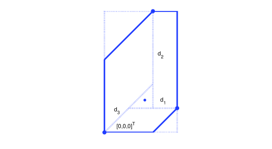
Figure 15: Looking for $d,d_{1},d_{2},d_{3}$ in the proof of lemma 4 , with $t_{21}\leq t_{12}$.

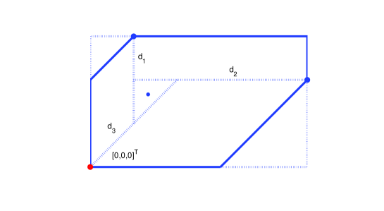
Figure 16: Looking for $d,d_{1},d_{2},d_{3}$ in the proof of lemma 4, with $t_{21}\geq t_{12}$.

Example 1.

Suppose that $A$ is idempotent normal with $t_{12}=t_{21}$ and $t_{11}=t_{22}$.

$$A_{0}=\left[\begin{array}[]{ccc}t_{11}&t_{12}&0\\ t_{12}&t_{11}&0\\ 0&0&0\end{array}\right].$$

Then $0\leq t_{12}\leq t_{11}$ and the new three points shown in figures 16 and 15 collapse to $[t_{12},t_{12},0]^{T}$. In this case $d=0$, $d_{1}=d_{2}=t_{11}-t_{12}$, $d_{3}=t_{12}$, $Q=\operatorname{diag}(d_{3},d_{3},0)$ and $L=Q^{\odot-1}\odot A\odot Q$ satisfies

$$L=\left[\begin{array}[]{ccc}0&t_{12}-t_{11}&-t_{12}\\ t_{12}-t_{11}&0&-t_{12}\\ t_{12}-t_{11}&t_{12}-t_{11}&0\\ \end{array}\right],\qquad L_{0}=\left[\begin{array}[]{ccc}t_{11}-t_{12}&0&-t_{12}\\ 0&t_{11}-t_{12}&-t_{12}\\ 0&0&0\\ \end{array}\right].$$

Notice that $P_{12}\odot L\odot P_{12}=L$.

Corollary 1.

A good tropical triangle is classically convex in $Z=0$.

Proof.

Let $\mathcal{T}_{A}$ be a good tropical triangle, for some matrix $A$. By the paragraph after (11), a translation allows us to assume that $A$ is normal. By lemmas 2 and 4, we can assume that $A=L(d,d_{1},d_{2},d_{3})$, for some $d,d_{1},d_{2},d_{3}\geq 0$. By lemma 3, $\mathcal{T}_{A}$ is determined by the columns of the matrices $A$ and $-A^{T}$ and, working in $Z=0$, we must look at the matrices $A_{0}$ and $(-A^{T})_{0}$ shown above in (21) and (22). Convexity immediately follows; see figure 13. ∎

Lemma 5.

Given $d,d_{1},d_{2},d_{3}\in\mathbb{R}$, $d\geq 0$, $-d\leq d_{j}$, for $j=1,2,3$, set $A=L(d,d_{1},d_{2},d_{3})$. The following are equivalent:

1. $A\neq A^{\odot 2}$,

2. $d_{j}<0$, for some $j=1,2,3$,

3. in $Z=0$, $\mathcal{T}_{A}$ is not classically convex.

Proof.

To check for convexity in $Z=0$, consider the matrix $A_{0}$ in expression (21). Say, $j=1$. If $d_{1}<0$, then any point in the classical segment $\overline{p,q}$, with $p=[d+d_{1},2d+d_{1}+d_{2},0]^{T}$ and $q=\operatorname{col}(A_{0},2)$, prevents $\mathcal{T}_{A}$ from being convex; see figure 17. ∎

Denote by $a$ the classical directed segment from $p$ to $q$, including $q$ and excluding $p$, as in the proof above. We will say that $a$ is an antenna of $\mathcal{T}_{A}$. The integer length of $a$ is $-d_{1}$ and the direction of $a$ is north–east. For $d_{2}<0$ (resp. $d_{3}<0$) we would get an antenna pointing west (resp. south).

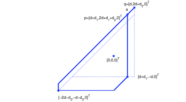
Figure 17: Tropical triangle with an antenna $a$ due to $d_{1}<0$.

In the hypothesis of the former lemma, $\mathcal{T}_{A}$ admits a cell decomposition having, at most, 13 cells (relatively open sets), and this is the generic case:

• one two–dimensional cell,

• six one–dimensional cells,

• six zero–dimensional cells.

Any one–dimensional cell disrupting the convexity of $\mathcal{T}_{A}$ in $Z=0$ gives rise to an antenna, as in [8]. Each antenna is the union of a one–dimensional cell and a zero–dimensional cell. The union of points in the antennas of $\mathcal{T}_{A}$ will be denoted $\operatorname{ant}(\mathcal{T}_{A})$. In lemma 5, we have shown that each $d_{j}<0$ yields an antenna in $\mathcal{T}_{A}$. The integer length of this antenna is $|d_{j}|$ and $|d_{j}|\leq d$.

Notice that this cell decomposition is not the same as the one associated to $A$, as defined on p. 8 and 2.

Corollary 2.

Given $d,d_{1},d_{2},d_{3}\in\mathbb{R}$, $d\geq 0$, $-d\leq d_{j}$, for $j=1,2,3$, set $A=L(d,d_{1},d_{2},d_{3})$. Then $\mathcal{T}_{A^{\odot 2}}=\mathcal{T}_{A}\setminus\operatorname{ant}(\mathcal{T}_{A})$, in $Z=0$.

Proof.

We know that $A$ is normal. If $A=A^{\odot 2}$, we just have corollary 1. Otherwise $A^{\odot 2}=(A^{\odot 2})^{\odot 2}$, by lemma 1, so that $\mathcal{T}_{A^{\odot 2}}$ is convex in $Z=0$, by lemma 2 and corollary 1. Now we compute

$$A^{\odot 2}=\left[\begin{array}[]{ccc}0&-d-d_{2}&-2d-d_{3}-d_{2}^{-}\\ -2d-d_{1}-d_{3}^{-}&0&-d-d_{3}\\ -d-d_{1}&-2d-d_{2}-d_{1}^{-}&0\\ \end{array}\right],$$ (23)

$$(A^{\odot 2})_{0}=\left[\begin{array}[]{ccc}d+d_{1}&d+d_{1}^{-}&-2d-d_{3}-d_{2}^{-}\\ -d-d_{3}^{-}&2d+d_{1}+d_{2}&-d-d_{3}\\ 0&0&0\\ \end{array}\right].$$ (24)

where $s^{-}=\min\{s,0\}$. If, say, $d_{1}<0$, then $\operatorname{col}((A^{\odot 2})_{0},2)=[d+d_{1},2d+d_{1}+d_{2},0]^{T}$ and $\operatorname{col}(A_{0},1)=[d+d_{1},-d,0]^{T}$ so that both points lie on the classical line $X=d+d_{1}$, meaning that the antenna in $\mathcal{T}_{A}$ caused by the inequality $d_{1}<0$ no longer appears in $\mathcal{T}_{A^{\odot 2}}$. ∎

The former corollary tells us that squaring the normal matrix $A=L(d,d_{1},d_{2},d_{3})$ corresponds to chopping off the antennas of $\mathcal{T}_{A}$, if any. The tropical triangle $\mathcal{T}_{A^{\odot 2}}$ will be called the soma of $\mathcal{T}_{A}$, denoted $\operatorname{soma}(\mathcal{T}_{A})$. Then

$$\mathcal{T}_{A}=\operatorname{soma}(\mathcal{T}_{A})\cup\operatorname{ant}(\mathcal{T}_{A})$$ (25)

is a disjoint union.

Notice that $A^{\odot 2}=0$ does not imply $A=0$, even if $A$ is normal. For example,

$$A=\left[\begin{array}[]{ccc}0&0&-\gamma\\ -\alpha&0&0\\ 0&-\beta&0\\ \end{array}\right],$$ (26)

with $\alpha,\beta,\gamma\geq 0$.

We know that the antennas (if any) of $\mathcal{T}_{A}$ have integer length $|d_{j}|\leq d$, when $A=L(d,d_{1},d_{2},d_{3})$ with $d\geq 0$ and $-d\leq d_{j}$. But, there exist tropical triangles with antennas of arbitrary length. Moreover, notice the way that antennas wrap around the two dimensional part of a triangle $\mathcal{T}_{A}$, for $A=L(d,d_{1},d_{2},d_{3})$ with $d>0$, $0<|d_{j}|<d$, $j=1,2$ and compare with the essentially different way that antennas wrap around the two dimensional part of the triangle $\mathcal{T}_{B}$ (see figure 19), for

$$B=\left[\begin{array}[]{rrr}0&-5&0\\ -7&0&0\\ -6&-1&0\end{array}\right],\qquad B_{0}=\left[\begin{array}[]{rrr}6&-4&0\\ -1&1&0\\ 0&0&0\end{array}\right].$$ (27)

For these two reasons, in order to find a canonical normalization for the matrices describing these triangles, we must consider matrices more general than $L(d,d_{1},d_{2},d_{3})$.

Consider

$$F(d,d_{1},d_{2},d_{3},h_{1},h_{2},h_{3},g)=\left[\begin{array}[]{ccc}0&-d-d_{2}&-2d-d_{3}-h_{3}\\ -2d-d_{1}-h_{1}&0&-d-d_{3}-g\\ -d-d_{1}&-2d-d_{2}-h_{2}&0\\ \end{array}\right],$$ (28)

with $d,d_{1},d_{2},d_{3},h_{1},h_{2},h_{3},g\geq 0$ such that

condition 1:

$h_{j+1}>0$ implies $d_{j}=0$,

condition 2:

$g>0$ implies $d=d_{1}=h_{3}=0$,

where all subscripts work modulo 3. Notice how the positivity of some of the parameters inhibit the positivity of other parameters. For pictures in $Z=0$, we will use

$$F(d,d_{1},d_{2},d_{3},h_{1},h_{2},h_{3},g)_{0}=\left[\begin{array}[]{ccc}d+d_{1}&d+h_{2}&-2d-d_{3}-h_{3}\\ -d-h_{1}&2d+d_{2}+h_{2}&-d-d_{3}-g\\ 0&0&0\\ \end{array}\right],$$ (29)

$$(-F(d,d_{1},d_{2},d_{3},h_{1},h_{2},h_{3},g)^{T})_{0}=\left[\begin{array}[]{ccc}-2d-d_{3}-h_{3}&d+d_{1}-d_{3}+h_{1}-g&d+d_{1}\\ -d+d_{2}-d_{3}-h_{3}&-d-d_{3}-g&2d+d_{2}+h_{2}\\ 0&0&0\\ \end{array}\right].$$ (30)

Notice that

• $F(d,d_{1},d_{2},d_{3},0,0,0,0)=L(d,d_{1},d_{2},d_{3})$.

• $F=F(d,d_{1},d_{2},d_{3},h_{1},h_{2},h_{3},g)$ is normal and $F^{\odot 2}=L(d,d_{1},d_{2},d_{3})$.

Theorem 1 (Lower canonical normalization).

If $A$ is any $3\times 3$ real matrix, then there exist unique $d,d_{1},d_{2},d_{3},h_{1},h_{2},h_{3},g\geq 0$ and there exist permutation matrices $P,Q$ such that $F(d,d_{1},d_{2},d_{3},h_{1},h_{2},h_{3},g)=P\odot A\odot Q$, where all subscripts work modulo 3.

Proof.

To prove existence, we may assume that $A$ is normal. If $A=A^{\odot 2}$, we take $h_{j}=g=0$, for all $j$, and apply lemma 4. Now assume that $A\neq A^{\odot 2}$. By the same lemma, we can assume that $A^{\odot 2}=L(d,d_{1},d_{2},d_{3})$, for some $d,d_{1},d_{2},d_{3}\geq 0$. In other words, $A$ is a tropical square root of $L(d,d_{1},d_{2},d_{3})$. The geometric meaning of this assertion is that $\mathcal{T}_{A}$ is obtained from $\mathcal{T}_{A^{\odot 2}}$ by pasting of antennas. Each antenna of $\mathcal{T}_{A}$ emanate from a vertex of $\mathcal{T}_{A^{\odot 2}}$, i.e., from the point represented by a column of $A^{\odot 2}$. At each vertex of $\mathcal{T}_{A^{\odot 2}}$, an antenna can be glued, at most.

Write

$$p=\operatorname{col}(A^{\odot 2},1),\quad q=\operatorname{col}(A^{\odot 2},2),\quad r=\operatorname{col}(A^{\odot 2},3),$$ (31)

$$p^{\prime}=\operatorname{col}(A,1),\quad q^{\prime}=\operatorname{col}(A,2),\quad r^{\prime}=\operatorname{col}(A,3).$$ (32)

Claim.

For $\mathcal{T}_{A^{\odot 2}}$ to admit gluing of antennas, it is necessary that the points $p$, $q$, $r$, $-(p\otimes q)$, $-(q\otimes r)$ and $-(r\otimes p)$ are NOT all different. In particular, $d_{j}=0$, for some $j$.

Indeed, suppose a small antenna $a$ emanates from $r$; this means that $r^{\prime}$ is perturbation of $r$. Let us work in $Z=0$. Recalling the rays of an affine tropical line, this antenna can point either west or south. Suppose that $a$ points west. Then $r^{\prime}=[-2d-d_{3}-\epsilon,-d-d_{3},0]^{T}$ and $\epsilon>0$ is the integer length of $a$. Consider the slope–one classical line through $q=[q_{1},q_{2},0]^{T}$, with equation $Y-X=q_{2}-q_{1}$, and the slope–zero line through $r=[r_{1},r_{2},0]^{T}$, with equation $Y=r_{2}$. These lines meet at the point $i=[r_{2}-q_{2}+q_{1},r_{2},0]^{T}$. Now $r_{2}-q_{2}+q_{1}\leq r_{1}$, since $\mathcal{T}_{A^{\odot 2}}$ is a good triangle (the former inequality is just another way of writing $a_{12}-a_{22}\leq a_{13}-a_{23}$ in (4)). For the antenna $a$ to exist, $r^{\prime}$ must be west of $i$ and for $a$ to emanate from $r$, it must happen that $i=r$, or equivalently, $r=-(q\otimes r)$. A simple computation shows that $-(q\otimes r)=[-2d-d_{3},-d-d_{3}+d_{2},0]^{T}$, so that $d_{2}=0$; see figure 19.

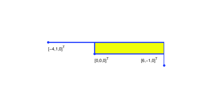
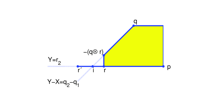
Figure 18: The tropical triangle corresponding to matrix $B$ in (27).

Figure 19: The three points $i,r$ and $-(q\otimes r)$ will collapse together.

Suppose now that $a$ points south. Then $r^{\prime}=[-2d-d_{3},-d-d_{3}-\epsilon,0]^{T}$ and $\epsilon>0$ is the integer length of $a$. In this case the points $r$ and $-(r\otimes p)$ coincide. A simple computation shows that $-(r\otimes p)=[d+d_{1}-d_{3},-d-d_{3},0]^{T}$. It follows that $d_{1}=-3d$, whence $d=d_{1}=0$. In particular, $p=[0,0,0]^{T}$.

The proof of the claim is similar, when $a$ emanates from $p$ or $q$.

• Assume $A^{\odot 2}=0$, i.e., $d=d_{1}=d_{2}=d_{3}=0$. Then, all the columns of $A^{\odot 2}$ represent the same point (the origin) and $\mathcal{T}_{A}$ is the union of the origin and, at most, three antennas, of integer lengths $h_{1},h_{2},h_{3}\geq 0$. Take then $g=0$ to get $A=F(0,0,0,0,h_{1},h_{2},h_{3},0)$.

• Assume now that the columns of $A^{\odot 2}$ represent three different points. Then, either $d\neq 0$ or $d=0$ and $d_{j}\neq 0\neq d_{j+1}$, for some $j$.

  We consider here matrices a bit more general than $F(d,d_{1},d_{2},d_{3},h_{1},h_{2},h_{3},g)$. Write $G(d,d_{1},d_{2},d_{3},h_{1},h_{2},h_{3},g_{1},g_{2},g_{3})=$

  $$\left[\begin{array}[]{ccc}0&-d-d_{2}-g_{2}&-2d-d_{3}-h_{3}\\ -2d-d_{1}-h_{1}&0&-d-d_{3}-g_{3}\\ -d-d_{1}-g_{1}&-2d-d_{2}-h_{2}&0\\ \end{array}\right]$$ (33)

  such that $d,d_{1},d_{2},d_{3},h_{1},h_{2},h_{3},g_{1},g_{2},g_{3}\geq 0$ and

  1. $h_{j+1}>0$ implies $d_{j}=g_{j+1}=0$,

  2. $g_{j}>0$ implies $d=d_{j+1}=h_{j}=0$,

  where all subscripts work modulo 3. A simple computation shows that $L(d,d_{1},d_{2},d_{3})$ equals $G(d,d_{1},d_{2},d_{3},h_{1},h_{2},h_{3},g_{1},g_{2},g_{3})^{\odot 2}$.

  Suppose that $A=G(d,d_{1},d_{2},d_{3},h_{1},h_{2},h_{3},g_{1},g_{2},g_{3})$.

  1. Say, $\mathcal{T}_{A}$ has an antenna $a$ of integer length $\epsilon$ emanating from the point represented by a column of $A^{\odot 2}$. Say this column is $r$.

     1. If $a$ points south, then $d=d_{1}=0$ and $p=[0,0,0]^{T}$. Take $g_{3}=\epsilon$ and $h_{3}=0$.

     2. If $a$ points west, then $d_{2}=0$. Take $g_{3}=0$ and $h_{3}=\epsilon$.

  2. Say, $\mathcal{T}_{A}$ has two antennas $a$ and $b$, and $a$ is emanating from $r$. Looking at the previous item, we see that only three cases are possible:

     1. If $g_{3}>0$, $d=d_{1}=h_{3}=0$ and $h_{2}>0$, $d_{1}=g_{2}=0$, so that $h_{2}$ is the integer length of $b$. The antenna $a$ points south and $b$ points north–east from $q$; see figure 21, left,

     2. If $h_{3}>0$, $d_{2}=g_{3}=0$ and $h_{2}>0$, $d_{1}=g_{2}=0$, so that $h_{2}$ is the integer length of $b$. The antenna $a$ points west and $b$ points north–east from $q$; see figure 21, center,

     3. If $h_{3}>0$, $d_{2}=g_{3}=0$ and $h_{1}>0$, $d_{3}=g_{1}=0$, so that $h_{1}$ is the integer length of $b$. The antenna $a$ points west and $b$ points south from $p$; see figure 21, right.

     

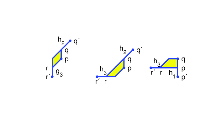
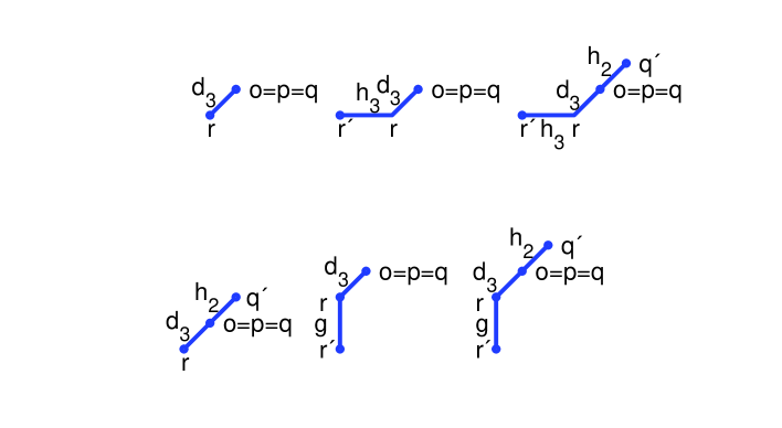
     Figure 20: All tropical triangles with two antennas (up to change of coordinates).

     

     Figure 21: All tropical triangles having 1–dimensional somas (up to change of coordinates).

     If we had $g_{3}>0$ and $g_{2}>0$, then $d=d_{1}=d_{3}=0$, contradicting that the columns of $A^{\odot 2}$ represent three different points. Similarly, if $g_{3}>0$ and $g_{1}>0$, or if $g_{2}>0$ and $g_{1}>0$.

  3. Say, $\mathcal{T}_{A}$ has three antennas. Then, by the previous item, the only possibility is $h_{1},h_{2},h_{3}>0$, so that $d_{j}=g_{j+1}=0$, for all $j$.

  We have just proved that $g_{j}>0$ is possible for only one value of $j=1,2,3$. Then, a change of coordinates allows us to assume $j=3$, and write $g_{3}=g$, so that $G(d,d_{1},d_{2},d_{3},h_{1},h_{2},h_{3},0,0,g)=F(d,d_{1},d_{2},d_{3},h_{1},h_{2},h_{3},g)$.

• Assume now that the columns of $A^{\odot 2}$ represent two different points. This case can be viewed as a degeneration of the previous cases, as $d>0$ tends to zero. Say $d=d_{1}=d_{2}=0$ and $d_{3}\neq 0$. Then $p=q$ is the origin and $h_{1}=0$. Here $\operatorname{soma}(\mathcal{T}_{A})$ reduces to a classical segment ; see figure 21.

So far, we have proved that given any $3\times 3$ matrix $A$, there exist permutation matrices $P,Q$ such that

$$F(d,d_{1},d_{2},d_{3},h_{1},h_{2},h_{3},g)^{\odot 2}=L(d,d_{1},d_{2},d_{3})=P\odot A^{\odot 2}\odot Q.$$

It turns out that the same matrices $P,Q$ provide

$$F(d,d_{1},d_{2},d_{3},h_{1},h_{2},h_{3},g)=P\odot A\odot Q.$$

The uniqueness of $d,d_{1},d_{2},d_{3},h_{1},h_{2},h_{3},g$ follows from the geometric meaning of these parameters. ∎

Corollary 3.

$F(d,d_{1},d_{2},d_{3},h_{1},h_{2},h_{3},g)$ is a tropical square root of $L(d,d_{1},d_{2},d_{3})$.∎

Example 2.

Let us compute the lower canonical normalization of

$$A=A_{0}=\left[\begin{array}[]{ccc}0&1&3\\ 0&3&4\\ 0&0&0\\ \end{array}\right],$$

the example in [8], p. 409. Consider the matrices $U=\operatorname{diag}(-1,0,0)$,

$$Q=\left[\begin{array}[]{ccc}-\infty&-\infty&0\\ 0&-\infty&-\infty\\ -\infty&0&-\infty\end{array}\right]$$

and obtain

$$N_{0}=U\odot P_{12}\odot A\odot Q=\left[\begin{array}[]{ccc}2&3&-1\\ 1&3&0\\ 0&0&0\end{array}\right].$$

Then

$$N=N_{0}\odot\operatorname{diag}(-2,-3,0)=\left[\begin{array}[]{ccc}0&0&-1\\ -1&0&0\\ -2&-3&0\end{array}\right]$$

is normal. Then

$$N^{\odot 2}=\left[\begin{array}[]{ccc}0&0&0\\ -1&0&0\\ -2&-2&0\end{array}\right],\qquad(N^{\odot 2})_{0}=\left[\begin{array}[]{ccc}2&2&0\\ 1&2&0\\ 0&0&0\end{array}\right].$$

In figure 22, we find, from left to right, the tropical triangles corresponding to the matrices $A,P_{12}\odot A,U\odot P_{12}\odot A$, $U\odot P_{12}\odot A\odot Q$ and $N$ (the last three matrices yield the same triangle), all in $Z=0$. Here $3d=1$, $d_{1}=d_{2}=0$ and $d_{3}=1$ so that the lower canonical normalization of $N^{\odot 2}$ is

$$L\left(1/3,0,0,1\right)=\left[\begin{array}[]{ccc}0&-1/3&-5/3\\ -2/3&0&-4/3\\ -1/3&-2/3&0\end{array}\right]=S^{\odot-1}\odot N^{\odot 2}\odot S,$$

with $S=\operatorname{diag}(5/3,4/3,0)$. Thus, the lower canonical normalization of $A$ is

$$S^{\odot-1}\odot N\odot S=F\left(1/3,0,0,1,0,1,1,0\right)=\left[\begin{array}[]{ccc}0&-1/3&-8/3\\ -2/3&0&-4/3\\ -1/3&-5/3&0\end{array}\right].$$

We have $h_{1}=0$, $h_{2}=h_{3}=1$. For pictures in $Z=0$, we consider

$$L\left(1/3,0,0,1\right)_{0}=\left[\begin{array}[]{ccc}1/3&1/3&-5/3\\ -1/3&2/3&-4/3\\ 0&0&0\end{array}\right]$$

and

$$F\left(1/3,0,0,1,0,1,1,0\right)_{0}=\left[\begin{array}[]{ccc}1/3&4/3&-8/3\\ -1/3&5/3&-4/3\\ 0&0&0\end{array}\right].$$

In figure 23 we see the triangles corresponding to the matrix $N^{\odot 2}$ and its lower canonical normalization, while in figure 24 we see the triangles of the matrix $N$ and its lower canonical normalization. Notice that the matrices $S^{\odot-1}$ and $S$ provide the lower canonical normalization of $N^{\odot 2}$ and also of $N$.

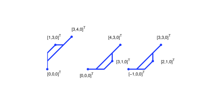
Figure 22: Tropical triangles $\mathcal{T}_{A}$, $\mathcal{T}_{P_{12}\odot A}$ and $\mathcal{T}_{N}$.

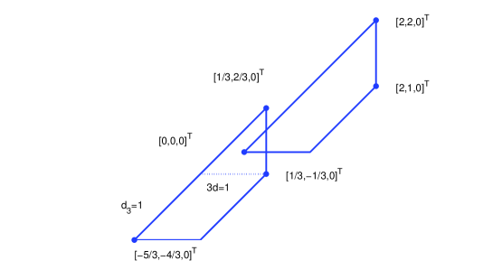
Figure 23: Tropical triangle corresponding to $N^{\odot 2}$ and to its lower canonical normalization.

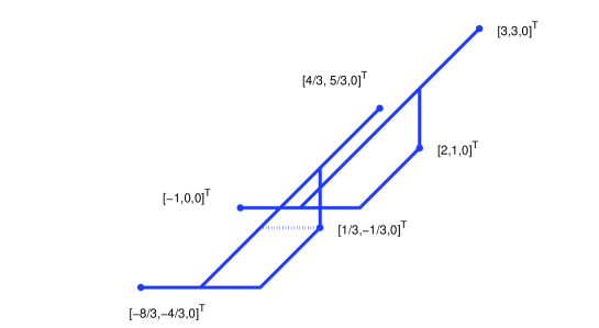
Figure 24: Tropical triangle corresponding to $N$ and to its lower canonical normalization.

Consider $A=F(d,d_{1},d_{2},d_{3},h_{1},h_{2},h_{3},g)$. Now, a definition of soma and antennas of $\mathcal{T}_{A}$ can be given, as in p. 17. The soma of $\mathcal{T}_{A}$ is $\mathcal{T}_{L(d,d_{1},d_{2},d_{3})}$. The antennas of $\mathcal{T}_{A}$ have tropical length $h_{j}$, if $h_{j}>0$ or $g$, if $g>0$.

For any $3\times 3$ matrix $A$ let $N=F(d,d_{1},d_{2},d_{3},h_{1},h_{2},h_{3},g)$ be the lower canonical normalization of $A$. There exist permutation matrices $P,Q$ such that $N=P\odot A\odot Q.$ The map $f_{P}$ is a translation, so that the triangle $\mathcal{T}_{A}=f_{P^{\odot-1}}(\mathcal{T}_{N})$ is just a translated of $\mathcal{T}_{N}$. Then we define the soma and antennas of $\mathcal{T}_{A}$ as follows:

$$\operatorname{soma}(\mathcal{T}_{A})=f_{P^{\odot-1}}(\operatorname{soma}\mathcal{T}_{N}),\qquad\operatorname{ant}(\mathcal{T}_{A})=f_{P^{\odot-1}}(\operatorname{ant}\mathcal{T}_{N}),$$ (34)

so that the decomposition (38) holds true, for any $A$.

The following theorem is a simple geometric characterization of normality.

Theorem 2.

The $3\times 3$ matrix $A$ is normal if and only if the origin belongs to $\operatorname{soma}(\mathcal{T}_{A})$, in $Z=0$.

Proof.

Recall expression (14). If $A$ is normal then $A^{\odot 2}$ is idempotent normal, so that $\operatorname{soma}(\mathcal{T}_{A})$ is a good triangle. By expression (5), in $Z=0$ we have $\operatorname{soma}(\mathcal{T}_{A})=\mathcal{T}$, for some $a,b,c,d,e,f\in\mathbb{R}$. Then

$$c-f\leq x\leq d-e,\ a+e\leq y\leq b+f,\ c-b\leq y-x\leq d-a.$$ (35)

If we write

$$\overline{a}=a\oplus(c-f),\quad\overline{c}=c\oplus(a+e),\quad\overline{e}=e\oplus(c-b),$$

$$\overline{b}=b\oplus^{\prime}(d-e),\quad\overline{d}=d\oplus^{\prime}(b+f),\quad\overline{f}=f\oplus^{\prime}(d-a),$$

then

$$\operatorname{soma}(\mathcal{T}_{A})=\{(x,y)\in\mathbb{R}^{2}:\overline{a}\leq x\leq\overline{b},\ \overline{c}\leq y\leq\overline{d},\ \overline{e}\leq y-x\leq\overline{f}\}$$ (36)

and $\operatorname{soma}(\mathcal{T}_{A})$ is the set of points spanned by the columns of the idempotent matrix $B$, where

$$B=\left[\begin{array}[]{ccc}0&-\overline{f}&\overline{a}\\ \overline{e}&0&\overline{c}\\ -\overline{b}&-\overline{d}&0\end{array}\right],\quad B_{0}=\left[\begin{array}[]{ccc}\overline{b}&\overline{d}-\overline{f}&\overline{a}\\ \overline{b}+\overline{e}&\overline{d}&\overline{c}\\ 0&0&0\end{array}\right].$$ (37)

Then $B=A^{\odot 2}$, whence $\overline{a},\overline{c},\overline{e}\leq 0\leq\overline{b},\overline{d},\overline{f}$, by normality. Clearly the origin belongs to $\operatorname{soma}(\mathcal{T}_{A})$ in $Z=0$.

Conversely, if $\operatorname{soma}(\mathcal{T}_{A})$ is a point (the origin), then $A^{\odot 2}=0=L(0,0,0,0)$, whence $A=F(0,0,0,0,h_{1},h_{2},h_{3},g)$, for some $h_{1},h_{2},h_{3},g\geq 0$, showing that $A$ is normal. On the other hand, if $\operatorname{soma}(\mathcal{T}_{A})$ has dimension $\geq 1$ and contains the origin, then $\operatorname{col}((A^{\odot 2})_{0},j)\in\overline{C^{0}_{j}}$, for $j=1,2,3$. Now, gluing antennas (at most three, and in prescribed directions: north–east, west and south) to $\operatorname{soma}(\mathcal{T}_{A})$ provides $\mathcal{T}_{A}$. The end points of these antennas are precisely the columns of $A_{0}$ and $\operatorname{col}(A_{0},j)\in\overline{C^{0}_{j}}$, for $j=1,2,3$, showing normality of $A$. ∎

Example 3.

Let us look at example 2 again, (see fig. 25). A normalization of $A$ is $N=P\odot A\odot Q$, where $P=\operatorname{diag}(-2,-3,0)$,

$$N=\left[\begin{array}[]{ccc}0&-1&-2\\ 0&0&-3\\ -1&0&0\\ \end{array}\right],\qquad Q=\left[\begin{array}[]{ccc}-\infty&-\infty&0\\ -\infty&0&-\infty\\ -1&-\infty&-\infty\end{array}\right].$$

We have

$$N_{0}=\left[\begin{array}[]{ccc}1&-1&-2\\ 1&0&-3\\ 0&0&0\end{array}\right],\qquad N^{\odot 2}=\left[\begin{array}[]{ccc}0&-1&-2\\ 0&0&-2\\ 0&0&0\\ \end{array}\right]=(N^{\odot 2})_{0}.$$

Another normalization of $A$ is $N=P\odot A\odot Q,$ where $P=\operatorname{diag}(-1,-3,0)$,

$$N=\left[\begin{array}[]{ccc}0&0&-1\\ -1&0&-3\\ -2&0&0\\ \end{array}\right],\qquad Q=\left[\begin{array}[]{ccc}-\infty&-\infty&0\\ -\infty&0&-\infty\\ -2&-\infty&-\infty\end{array}\right];$$

in this case,

$$N_{0}=\left[\begin{array}[]{ccc}2&0&-1\\ 1&0&-3\\ 0&0&0\end{array}\right],\ N^{\odot 2}=\left[\begin{array}[]{ccc}0&0&-1\\ -1&0&-2\\ -1&0&0\\ \end{array}\right],\ (N^{\odot 2})_{0}=\left[\begin{array}[]{ccc}1&0&-1\\ 0&0&-2\\ 0&0&0\\ \end{array}\right].$$

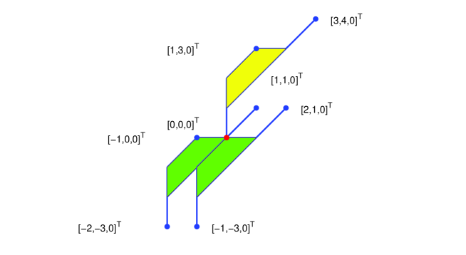
Figure 25: Tropical triangles $\mathcal{T}_{A}$ and $\mathcal{T}_{N}$, for two different normalizations $N$.

Next, we procede to define soma and antennas of a co–spanned tropical triangle. Regarding co–span, we choose to work with co–normal matrices, i.e., matrices $A$ having non–negative entries and zero diagonal. We can achieve a lower canonical co–normalization and then define soma and antennas of a co–spanned tropical triangle, in a similar fashion to theorem 1 and definition in p. 34. Since antennas of spanned triangles grow only in three directions (north–east, west and south), then antennas of co–spanned triangles grow only in three directions (south–west, east and north).

For a given matrix $A$, consider the triangle $\mathcal{T}^{A}=\operatorname{co--span}(-A^{T})$. Then

$$\mathcal{T}^{A}=\operatorname{soma}(\mathcal{T}^{A})\cup\operatorname{ant}(\mathcal{T}^{A})$$ (38)

is a disjoint union. Suppose that the two–dimensional cell $B^{A}$, as defined on p. 8, is non–empty. Then

$$\overline{B^{A}}=\operatorname{soma}(\mathcal{T}^{A}).$$ (39)

On the other hand, $B^{A}$ is empty if and only if $\operatorname{soma}(\mathcal{T}^{A})$ reduces to a segment or point.

Now, what is the relationship between $\mathcal{T}_{A}$ and $\mathcal{T}^{A}$, $\operatorname{soma}(\mathcal{T}_{A})$ and $\operatorname{soma}(\mathcal{T}^{A})$, $\operatorname{ant}(\mathcal{T}_{A})$ and $\operatorname{ant}(\mathcal{T}^{A})$, for a given normal matrix $A=F(d,d_{1},d_{2},d_{3},h_{1},h_{2},h_{3},g)$?

• If $h_{1}=h_{2}=h_{3}=0$, then $A$ is idempotent normal. By lemma 2, $\mathcal{T}_{A}$ is good, so that the columns of $-A^{T}$ are precisely the vertices of the sides of $\mathcal{T}_{A}$, see figure 13. By the max–min duality, the columns of $A$ are the stable intersection points of the tropical lines $A_{1},A_{2},A_{3}$. Therefore,

  $$\operatorname{soma}(\mathcal{T}_{A})=\mathcal{T}_{A}=\operatorname{span}(A)=\operatorname{co--span}(-A^{T})=\mathcal{T}^{A}=\operatorname{soma}(\mathcal{T}^{A}).$$ (40)

• If $h_{j+1}>0$ and $d_{j}=0$ for some $j$, by the previous item,

  $$\operatorname{soma}(\mathcal{T}_{A})=\mathcal{T}_{A^{\odot 2}}=\mathcal{T}^{A^{\odot 2}}=\operatorname{soma}(\mathcal{T}^{A}),$$ (41)

  even though $\mathcal{T}_{A}\neq\mathcal{T}^{A}$.

  Write $S=\operatorname{soma}(\mathcal{T}_{A})$. Each antenna $a$ of $\mathcal{T}_{A}$ grows at a vertex $v$ of $S$. An antenna $a^{\prime}$ of $\mathcal{T}^{A}$ grows at $v$, as well and, in fact, the integer length of $a$ and $a^{\prime}$ is the same. We claim that there exists a unique two–dimensional peripheral cell, denoted $P_{a}$, in the cell decomposition $\mathcal{C}^{A}$ such that $a^{\prime}\cup a\subset\overline{P_{a}}$. Indeed, by hypothesis, $A=F(d,d_{1},d_{2},d_{3},h_{1},h_{2},h_{3},g)$ and $A^{\odot 2}=L(d,d_{1},d_{2},d_{3})$, for some $d,d_{1},d_{2},d_{3},h_{1},h_{2},h_{3},g\geq 0$ with $h_{j+1}>0$ implying $d_{j}=0$ and $g>0$ implying $d=d_{1}=h_{3}=0$. Say $h_{2}>0$, $d_{1}=0$ so that $\mathcal{T}_{A}$ has an antenna $a$ pointing north–east (see figure 26). Looking at (21), (29) and (30) we know that the end points of $a$ are $v=\operatorname{col}((A^{\odot 2})_{0},2)=[d,2d+d_{2},0]^{T}$ and $\operatorname{col}(A_{0},2)=[d+h_{2},2d+d_{2}+h_{2},0]^{T}$ while the end points of $a^{\prime}$ are $v$ and $\operatorname{col}((-A^{T})_{0},3)=[d,2d+d_{2}+h_{2},0]^{T}$. Therefore, we have the following expression of $P_{a}$ in $Z=0$:

  $$P_{a}=\{(x,y)^{T}\in\mathbb{T}^{2}:d<x,\quad 0<y-x-d-d_{2}<h_{2}\}.$$ (42)

• If $A=F(0,0,d_{2},d_{3},0,h_{2},0,g)$, with $d_{2},d_{3}\geq 0$, $g>0$, then $\mathcal{T}_{A}$ has an antenna $a$ of integer length $g$ emanating from $\operatorname{col}(A^{\odot 2},3)$. Computing $(-A^{T})_{0}$ we see that $\mathcal{T}^{A}$ has an antenna $a^{\prime}$ of the same integer length, emanating from the same point. The corresponding peripheral cell $P_{a}$ is expressed as follows in $Z=0$:

  $$P_{a}=\{(x,y)\in\mathbb{T}^{2}:-d_{3}-g<x<-d_{3},\ y<x\}.$$ (43)

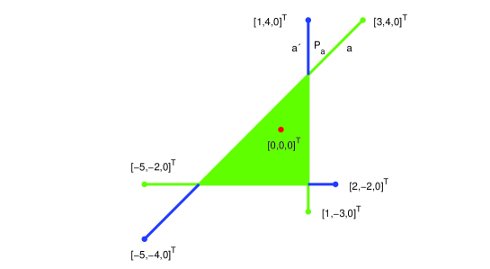
Figure 26: Tropical triangles $\mathcal{T}_{A}$, $\mathcal{T}^{A}$, antennas $a$ and $a^{\prime}$ and the two–dimensional cell $P_{a}$, for $A$ in (9).

5 The map $f_{A}$ for a $A=F(d,d_{1},d_{2},d_{3},h_{1},h_{2},h_{3},g)$

Recall that $\overline{\Gamma}$ denotes the closure of $\Gamma\subseteq\mathbb{T}\mathbb{P}^{2}$. The following theorem fully describes the action of the map $f_{A}$ on each point of $\mathbb{T}\mathbb{P}^{2}$, since $\mathbb{T}\mathbb{P}^{2}$ is a (finite) union of $\overline{\Gamma}$, where $\Gamma$ is a two–dimensional cell in $\mathcal{C}^{A}$. The cell $\Gamma$ is of the following types: either $B^{A}$ (central cell), or $P_{a}$ (peripheral cell parallel to some coordinate axis, associated to some antenna $a$), or $P$ (peripheral cell parallel to some coordinate axis, not associated to any antenna) or $C$ (corner). The cell $B^{A}$ can be empty. If $A=F(d,d_{1},d_{2},d_{3},h_{1},h_{2},h_{3},g)$, then $B^{A}=\emptyset$ if and only if $d=d_{j}=d_{j+1}=0$, for some $j$ modulo 3.

Theorem 3.

Let $A=F(d,d_{1},d_{2},d_{3},h_{1},h_{2},h_{3},g)$ be given. Then

1. $f_{A}|_{\overline{C}}$ collapses to some vertex of $\mathcal{T}_{A}$, for every corner $C$ in $\mathcal{C}^{A}$,

2. $f_{A}|_{\overline{P_{a}}}=a$, for every antenna $a$ of $\mathcal{T}_{A}$,

3. $f_{A}|_{\overline{P}}$ is the classical projection onto $\mathcal{T}_{A}$, in the direction of $P$, for every two–dimensional peripheral cell $P$ of $\mathcal{C}^{A}$, if $P\neq P_{a}$, for every $a$ antenna of $\mathcal{T}_{A}$,

4. $\operatorname{soma}(\mathcal{T}_{A})$ is the set of fixed points of $f_{A}$ and, if $B^{A}\neq\emptyset$, then $\operatorname{soma}(\mathcal{T}_{A})=\overline{B^{A}}$.

Proof.

$f_{A}$ is continuous, so that $f_{A}|_{\overline{\Gamma}}$ is easily computed from $f_{A}|_{\Gamma}$. Part (1) was proved in p. 2.

• Suppose that $h_{1}=h_{2}=h_{3}=0$. Then $A=L(d,d_{1},d_{2},d_{3})$ is idempotent normal. Since $\mathcal{T}_{A}$ is a tropical triangle without antennas, then part (2) does not apply. In order to prove part (3), let us work in $Z=0$. We have

  $$A_{0}=\left[\begin{array}[]{ccc}d+d_{1}&d&-2d-d_{3}\\ -d&2d+d_{2}&-d-d_{3}\\ 0&0&0\\ \end{array}\right],$$

  $$(-A^{T})_{0}=\left[\begin{array}[]{ccc}-2d-d_{3}&d+d_{1}-d_{3}&d+d_{1}\\ -d+d_{2}-d_{3}&-d-d_{3}&2d+d_{2}\\ 0&0&0\end{array}\right].$$

  Let $P$ be a peripheral cell in $\mathcal{C}^{A}$; say, $P$ is parallel to the $Y$ direction. Then either

  $$P=\{(x,y)^{T}\in\mathbb{T}^{2}:-2d-d_{3}<x<d+d_{1}-d_{3},\quad y<-d-d_{3}\}$$ (44)

  or

  $$P=\{(x,y)^{T}\in\mathbb{T}^{2}:d+d_{1}-d_{3}<x<d+d_{1},\quad y<x-2d-d_{1}\}.$$ (45)

  In the former case, $f_{A}(p)=[x,{-d-d_{3}},0]^{T}$; in the latter, $f_{A}(p)=[x,{x-2d-d_{1}},0]^{T}$. We can be more concise: if $p=[x,y,0]^{T}\in P$, then either $y=-\infty$ or $y\in\mathbb{R}$ is big and negative. Therefore, $f_{A}(p)=A\odot p$ is a tropical linear combination only of $c_{1}=\operatorname{col}(A,1)$ and $c_{3}=\operatorname{col}(A,3)$; in particular, $f_{A}(p)$ belongs to the tropical segment $\operatorname{span}(c_{1},c_{3})\subseteq\mathcal{T}_{A}$ (and $f_{A}(p)$ does not depend on $y$). This proves part (3).

  By lemma 1, each point in $\operatorname{span}(A^{\odot 2})=\operatorname{soma}(\mathcal{T}_{A})$ is fixed by $f_{A}$. From equality (39) and parts (3), (2) and (1), now part (4) follows.

• Suppose that $h_{j+1}>0$ and $d_{j}=0$, for some $j$; say $j=2$ and $P_{a}$ is given in (42). For any $p=[x,y,0]^{T}\in\overline{P_{a}}$ we have $f_{A}(p)=[y-d-d_{2},y,x-d]^{T}=[y-x-d_{2},y-x+d,0]^{T}\in a$. In particular, $f_{A}(a^{\prime})=a$, where $a^{\prime}$ is the antenna of $\mathcal{T}^{A}$ corresponding to $a$. This proves part (2). Parts (3) and (4) are proved as in the previous case.

• Suppose that $g>0$ and $d=d_{1}=h_{3}=0$. Then $P_{a}$ is given in (43). The proof is similar to the previous case.

∎

Remark 1.

If $A=L(d,d_{1},d_{2},d_{3})$ for $d,d_{1},d_{2},d_{3}\geq 0$, then $f_{A}=f_{A}\circ f_{A}$, by theorem 3, meaning that $f_{A}$ is some kind of projection. But, in general, $f_{A}$ is different from the projector map onto $\mathcal{T}_{A}$ in p. 9. For instance, consider the matrix $A=L(3,9,2,4)$, i.e.,

$$A=\left[\begin{array}[]{ccc}0&-5&-10\\ -15&0&-7\\ -12&-8&0\end{array}\right],\quad A_{0}=\left[\begin{array}[]{ccc}12&3&-10\\ -3&8&-7\\ 0&0&0\end{array}\right],\quad p=\left[\begin{array}[]{c}-12\\ 0\\ 0\end{array}\right].$$

Then

$$\rho(p)=\left[\begin{array}[]{c}-12\\ -27\\ -24\end{array}\right]\oplus\left[\begin{array}[]{c}-12\\ -7\\ -15\end{array}\right]\oplus\left[\begin{array}[]{c}-12\\ -9\\ -2\end{array}\right]=\left[\begin{array}[]{c}-12\\ -7\\ -2\end{array}\right]=\left[\begin{array}[]{c}-10\\ -5\\ 0\end{array}\right]$$

$$f_{A}(p)=\left[\begin{array}[]{c}-5\\ 0\\ 0\end{array}\right]\neq\rho(p).$$

The results above extend to two types of matrices over $\mathbb{T}$.

• If $A$ is a permutation matrix, then $I=L(0,\infty,\infty,\infty)$ can be conceived as the lower canonical normalization of $A$; $I$ can be viewed as the limit of $L(0,d_{1},d_{2},d_{3})$, as all the $d_{j}$’s tend to infinity. In this case, $\mathcal{T}_{A}=\mathcal{T}_{I}=\mathbb{T}\mathbb{P}^{2}$ and $f_{A}=f_{I}$ is the identity.

• If $A=D\odot P$ for some permutation matrix $P$ and

  $$D=\left[\begin{array}[]{ccc}-\infty&0&0\\ 0&-\infty&0\\ 0&0&-\infty\\ \end{array}\right],$$ (46)

  then $N=F(0,0,0,0,\infty,\infty,\infty,0)$ can be considered the lower canonical normalization of $A$ and $N$ is, in some sense, the limit of $F(0,0,0,0,h_{1},h_{2},h_{3},0)$, as all the $h_{j}$’s tend to infinity; see (26). In this case, $\mathcal{T}_{A}$ is just the tropical line $L_{0}$ and $\operatorname{soma}(\mathcal{T}_{A})$ is the origin.

Neither $-I^{T}$ nor $-D^{T}$ can be written with entries in $\mathbb{T}$. However, according to the equivalence relation in p. 2, $[0,a,b]$ tends to $[-\infty,0,0]$ (resp. $[-\infty,0,-\infty]$) when $a,b\to\infty$ (resp. $a\to\infty$ and $b$ remains fixed), so that $D$ can be interpreted as $-I^{T}$.

If $A$ is a permutation matrix or $A=D\odot P$, then the cell decomposition $\mathcal{C}^{A}$ is obvious.

Definition 1.

A $3\times 3$ matrix $A$ is admissible if either $A$ is real or $A=B\odot P$, where $B=D$ in (46) or $B=I$ and $P$ is a permutation matrix.

Finally, we can describe the map $f_{A}$, for any $3\times 3$ admissible matrix $A$. First, we find the lower canonical normalization $N=F(d,d_{1},d_{2},d_{3},h_{1},h_{2},h_{3},g)=P\odot A\odot Q$ to obtain $f_{N}=f_{P}\circ f_{A}\circ f_{Q}$; then we apply theorem 3, knowing that $f_{P}$ and $f_{Q}$ are just changes of coordinates.

Consider the set $S_{A}$ of points where $f_{A}$ is injective, i.e.,

$$S_{A}=\{q\in\mathbb{T}\mathbb{P}^{2}:\exists\ !\ p\in\mathbb{T}\mathbb{P}^{2},f_{A}(p)=q\}.$$

On $\mathbb{R}^{n}$, the set $S_{A}$ plays an important role in [6].

Suppose that $A$ is admissible. If $A=P$ is a permutation matrix, then $S_{A}=\mathbb{T}\mathbb{P}^{2}$. If $A=D\odot P$, then $S_{A}$ reduces to the origin. If $A$ is real and $A=F(d,d_{1},d_{2},d_{3},h_{1},h_{2},h_{3},g)$, then $S_{A}=B^{A}$, by theorem 3 and equality (39). And if $N=P\odot A\odot Q$ is the lower canonical normalization of $A$, then $S_{A}=S_{A\odot Q}=f_{P^{\odot-1}}(B^{N})=B^{A}$. In other words, $f_{A}$ is injective precisely on $B^{A}$, when $A$ is real.

Corollary 4.

If $A$ is an admissible matrix, then $f_{A}$ transforms tropical collinear points into tropical collinear points.

Proof.

All we need to show is that the image of a tropical line $L\subset\mathbb{T}\mathbb{P}^{2}$ is contained in some tropical line $L^{\prime}$. Now, the cell decomposition $\mathcal{C}^{A}$ on $\mathbb{T}\mathbb{P}^{2}$ induces a cell decomposition on $L$. The triangle $\mathcal{T}_{A}$ is also decomposed into cells. Now, a case by case analysis (depending on the position of the vertex of $L$) and theorem 3, shows that each cell $\Gamma$ of $L$ is mapped by $f_{A}$ inside a cell $\Gamma^{\prime}$ of $\mathcal{T}_{A}$. And the union of all such $\Gamma^{\prime}$’s is contained in a tropical line $L^{\prime}$. ∎

References

[1]
[1] M. Akian, R. Bapat and S. Gaubert, Max–plus algebra, chapter 25 in Handbook of linear algebra, L. Hobgen (ed.) Chapman and Hall, 2007.
[2] M. Akian, S. Gaubert and C. Walsh, Discrete max–plus spectral theory, in [18], 53–77.
[3] M. Ansola and M.J. de la Puente, A note on tropical triangles in the plane, Acta Math. Sinica (Engl. ser.), 25, n. 11, (2009), 1775–1786.
[4] F.L. Baccelli, G. Cohen, G.J. Olsder and J.P. Quadrat, Syncronization and linearity, John Wiley; Chichester; New York, 1992.
[5] J.F. Barbero, Transformaciones
en el plano tropical, Trabajo de
investigación, Facultad de Matemáticas, UCM,
(2007).
[6] P. Butkovič, Simple image set of linear mappings, Discrete Appl. Math., 105, (2000), 73–86.
[7] B. Carré, Graphs and networks, Clarendon Press, Oxford, 1979.
[8] G. Cohen, S. Gaubert and J.P. Quadrat, Duality and separation theorems in idempotent semimodules, Lineal Algebra Appl., 379, (2004), 395–422.
[9] R. Cuninghame–Green, Minimax algebra, LNEMS, 166, Springer, 1970.
[10] R. Cuninghame–Green, in Adv. Imag. Electr. Phys., 90, P. Hawkes, (ed.), Academic Press, 1995, 1–121.
[11] R.A. Cuninghame–Green,
P. Butkovič, Bases in max-algebra, Linear
Algebra Appl. 389, (2004) 107–120.
[12] M. Develin, B. Sturmfels,
Tropical convexity, Doc. Math., 9, (2004), 1–27; Erratum in Doc. Math. 9 (electronic),
205–206 (2004).
[13] A. Gathmann, Tropical algebraic
geometry, Jahresbericht der DMV, 108, n.1,
(2006), 3–32.
[14] S. Gaubert and Max Plus, Methods and applications of linear algebra,
in R. Reischuk and M. Morvan, (eds.), STACS’97, 1200 in LNCS, 261–282, Lübeck, March 1997, Springer.
[15] I. Itenberg, G. Mikhalkin and E. Shustin, Tropical algebraic geometry,
Birkhäuser, 2007.
[16] M. Joswig, B. Sturmfels and J. Yu, Affine buildings and tropical convexity, Albanian J. Math. 1, n.4, (2007) 187–211.
[17] H.W. Kuhn, The hungarian method for the assignment problem, Naval Res. Logist., 2, (1955), 83–97.
[19] G.L. Litvinov, S.N. Sergeev, (eds.)
Tropical and idempotent mathematics, Proceedings Moscow 2007, American
Mathematical Society, Contemp. Math. 495, (2009).
[20] G. Merlet, Semigroup of matrices acting on the max–plus projective space, in press, Linear Algebra Appl. (2009), doi:10.1016/j.laa.2009.03.029
[21] G. Mikhalkin, What is a tropical curve?, Notices AMS, April 2007, 511–513.
[22] C.H. Papadimitriou and K. Steiglitz, Combinatorial optimization: algorithms and complexity, Prentice Hall, 1982, and corrected unabridged republication by Dover, 1998.
[23] J. Richter–Gebert, B. Sturmfels, T.
Theobald, First steps in tropical geometry, in
[18], 289–317.
[24] B. Sturmfels, Solving systems of polynomial equations,
CBMS Regional Conference Series in Math.
97, AMS, Providence, RI, 2002.
[25] E. Wagneur, Moduloïds and
pseudomodules. Dimension theory, Discr. Math. 98
(1991) 57–73.
[26] M. Yoeli, A note on a generalization of boolean matrix theory, Amer. Math. Monthly 68, n.6,
(1961) 552–557.