Interference in the radiation
of two point-like charges

Abstract

Energy-momentum and angular momentum carried by electromagnetic field of two point-like charged particles arbitrarily moving in flat spacetime are presented. Apart from usual contributions to the Noether quantities produced separately by particles 1 and 2, the conservation laws contain also joint contribution due to the fields of both particles. The mixed part of Maxwell energy-momentum density is decomposed into bound and radiative components which are separately conserved off the world lines of particles. The former describes the deformation of electromagnetic clouds of “bare” charges due to mutual interaction while the latter defines the radiation which escapes to infinity. The bound terms contribute to particles’ individual 4-momenta while the radiative ones exert the radiation reaction. Analysis of energy-momentum and angular momentum balance equations results the Lorentz-Dirac equation as an equation of motion for a pointed charge under the influence of its own electromagnetic field as well as field produced by another charge.

PACS numbers: 03.50.De, 11.10.Gh, 11.30.Cp

1 Introduction

The most natural and widely accepted equation of motion for a charge when radiation reaction is taken into account is the Lorentz-Dirac equation [1]. This equation has been discussed mainly for the case of one charge in an external electromagnetic field. In the present paper we consider an isolated system of two point electric charges and their electromagnetic field. We study the electromagnetic energy-momentum and angular momentum radiated by charges; the study of energy-momentum and angular momentum balance equations implies the Lorentz-Dirac equation for more than one charge.

The dynamics of the entire system is governed by the action

$$I=\sum\limits_{a=1}^{2}\left(-m_{a}\int{\rm d}s_{a}\sqrt{-{\dot{z}}_{a}^{2}}+e_{a}\int{\rm d}s_{a}A_{a,\mu}{\dot{z}}_{a}^{\mu}\right)-\frac{1}{16\pi}\int{\rm d}^{4}yf_{\mu\nu}f^{\mu\nu},$$

where $f_{\mu\nu}=\sum_{a}(\partial_{\mu}A_{a,\nu}-\partial_{\nu}A_{a,\mu})$ is the total field generated by two charges. Charge $e_{a}$ moves on a world line $\zeta_{a}\in{\mathbb{M}}_{4}$ described by functions $z_{a}^{\mu}(s_{a})$ which give the particle’s coordinates as functions of proper time $s_{a}$; ${\dot{z}}_{a}^{\mu}:=dz_{a}^{\mu}/ds_{a}$ is the $a$-th four-velocity.

The action is invariant under the space-time translations and rotations which constitute the Poincaré group. This immediately implies conserved quantities which place stringent requirements on the dynamics of the system. They demand that the change in electromagnetic field momentum [2],

$$p^{\nu}_{\rm em}=\int_{\Sigma}{\rm d}\sigma_{\alpha}T^{\alpha\nu},$$ (1.1)

and angular momentum [2],

$$M^{\mu\nu}_{\rm em}=\int_{\Sigma}{\rm d}\sigma_{\alpha}\left(y^{\mu}T^{\alpha\nu}-y^{\nu}T^{\alpha\mu}\right),$$ (1.2)

should be balanced by a corresponding change in the total momentum and total angular momentum of the particles. (By ${\rm d}\sigma_{\alpha}$ we denote the vectorial surface element on a space-like hypersurface $\Sigma$.)

Since the Maxwell energy-momentum tensor density,

$$4\pi T^{\mu\nu}=f^{\mu\lambda}f^{\nu}{}_{\lambda}-1/4\eta^{\mu\nu}f^{\kappa\lambda}f_{\kappa\lambda},$$ (1.3)

is quadratic in the field and this field satisfies the superposition principle, the total electromagnetic field stress-energy tensor is

$$T^{\mu\nu}=T_{(1)}^{\mu\nu}+T_{(2)}^{\mu\nu}+T_{\rm int}^{\mu\nu},$$ (1.4)

where $a$-th particle density $T_{(a)}^{\mu\nu}$ is given by the expression (1.3) where “total” field strengths $f^{\mu\nu}$ are substituted by “individual” ones $f^{\mu\nu}_{(a)}$. The mixed term

$$4\pi T_{\rm int}^{\mu\nu}=f_{(1)}^{\mu\lambda}f_{(2)}^{\nu}{}_{\lambda}+f_{(2)}^{\mu\lambda}f_{(1)}^{\nu}{}_{\lambda}-1/4\eta^{\mu\nu}\left(f_{(1)}^{\kappa\lambda}f_{\kappa\lambda}^{(2)}+f_{(2)}^{\kappa\lambda}f_{\kappa\lambda}^{(1)}\right)$$ (1.5)

describes the joint contribution due to both fields.

In this paper we study radiation produced by an isolated system of two point electric charges and their electromagnetic field. Outgoing electromagnetic waves remove energy, momentum, and angular momentum from the sources which then undergo radiation reaction. The verification of conservation laws is not a trivial matter, since the interference contribution (1.7) involves divergent terms.

In the derivation of particle’s equation of motion, Dirac [1] evaluated the flux of electromagnetic energy-momentum over a narrow world tube surrounding the particle’s world line. The author substituted the components of the retarded Liénard-Wiechert field in the stress-energy tensor (1.3) inside the narrow tube. In 1970 Teitelboim [3] splits the “retarded” stress-energy tensor into the “bound” and “emitted” parts which are separately conserved off the world line of the particle. The author calculates the flow of energy-momentum out of the portion of Bhabha world tube [4] bounded by tilted spacelike hypersurfaces which are orthogonal to particle’s four-velocity at instants $\tau$ and $\tau+{\rm d}\tau$, respectively. Bound part, ${\hat{T}}_{\rm bnd}$, describes a rigid electromagnetic “cloud” which are permanently attached to the source and carried along with it. “Bare” charge and “cloud” constitute new entity: dressed charged particle. ${\hat{T}}_{\rm bnd}$ contributes into particle’s inertia: 4-momentum of dressed charge contains, apart from usual velocity term, also a term which is proportional to the square of charge $e_{a}$,

$$p_{a}^{\mu}=m_{a}u_{a}^{\mu}-\frac{2e_{a}^{2}}{3}a_{a}^{\mu}.$$ (1.6)

(Coulomb-like infinity stemming from the pointness of “bare” source is absorbed by the rest mass $m_{a}$ within the renormalization procedure.) Time derivative of the second term in eq.(1.6) is the well-known Schott term which describes a reversible form of emission and absorption of field energy, which never gets far from the point-like source. The radiative part, ${\hat{T}}_{\rm rad}$, yields the Larmor relativistic rate of radiated energy-momentum. It detaches itself from the charge and leads an independent existence. This rate together with the Schott term constitutes the Abraham radiation reaction vector. López and Villarroel [5] split the torque of the stress-energy tensor into bound and emitted components which possess analogous properties.

The results can be applied to the first and the second terms in the total electromagnetic field stress-energy tensor (1.4) which describe “individual” radiation contributions due to particles 1 and 2, respectively. The question is what part of the mixed density should be taken instead of (1.5) to describe the radiation which reaches to a very distant sphere?

Aguirregabiria and Bel [6] studied the interference part of energy-momentum,

$$p_{\rm int}^{\nu}=\int_{\Sigma}d\sigma_{\mu}T_{\rm int}^{\mu\nu}\,,$$ (1.7)

carried by electromagnetic field of two point charges. The authors prove the fundamental theorem that the mixed radiation rate does not depend on the shape of spacelike surface $\Sigma$ which is used to integrate the mixed part (1.5) of the Maxwell energy-momentum tensor density. For a prescribed plane motion of the charges the perturbation scheme is elaborated within the framework of predictive relativistic mechanics [7, 8]. The lowest approximation gives the well-known expression [9, p.214] for the dipole radiation of two point charges moving according to Coulomb’s law. In Ref. [10] the scheme is applied to the angular momentum carried by electromagnetic field of two point charges.

In the case of $N$ particles we would merely obtain as an obvious generalization of eq. (1.4) the sum of $N$ one-particle terms and the mixed contributions corresponding to $N(N-1)/2$ pairs of charges. Hence, the interference component dominates in the radiation from a bunch of identical charged particles (e.g., in free electron lasers). To evaluate the radiation of a relativistic $N$-body system, Klepikov [11] defines the center of a system of radiation events which allows to synchronize the instants at which electromagnetic waves emitted by different charges combine on a very distant sphere. Fourier analysis is applied to calculate the time and angular distributions of energy-momentum flux. The radiation of a bunch of charged particles moving in a uniform magnetic field is considered in detail.

The only exact solution is obtained by Rivera and Villarroel Ref. [12, eq.(3.27)]. The authors calculate the rate of radiation (including interference part) generated by two identical point charges rotating uniformly at opposite ends of a diameter, in a fixed circle. External fields which govern the strictly prescribed motions are constructed. The rate of radiation is evaluated via the retarded Liénard-Wiechert fields produced by the charges. Further [13] more general case of circular motion of two unlike charges in two coplanar and concentric circumferences is considered.

Note that nine years before the radiation by a system of two uniformly circling charges has been evaluated by Hnizdo [14] (see also discussion [15, 16]). The author concludes that “the power radiated by such a system equals exactly the rate at which work is done on the system by external force”.

In this paper we study the interference part of energy-momentum and angular momentum of electromagnetic field generated by two arbitrarily moving charges. We restrict ourselves to the retarded Liénard-Wiechert solutions; the advanced ones are rejected on the grounds of causality. In Section 2 we introduce coordinate system which makes relatively easy the calculation of the covariant 4-momentum radiated by interacting charges. The calculation is performed in Sections 3 and 4. We reveal divergence-free radiative part of the mixed density (1.5). It determines the radiation that escapes to infinity while the (short-range) bound part modifies individual 4-momenta (1.6) of dressed particles. The mixed part of radiated energy-momentum depends only on velocities, accelerations and the relative 4-position of the charges. In Section 5 we derive equations of motion of interacting charged particles. Analysis of energy-momentum and angular momentum balance equations results the well-known Lorentz-Dirac equation. In Section 6 we study symmetry properties of radiative energy-momentum and angular momentum which rely on invariance of action (1) under inversions of space and time axes. In Section 7 we discuss the results and implications.

2 “Interference” coordinate system

To perform the surface integration (1.7) of interference stress-energy tensor, an appropriate coordinate system is necessary. Such a coordinate system is introduced in Ref. [6]. It involves the evolution parameter $\lambda$ associated with an inertial observer; the surface of integration is a surface of constant $\lambda$. In Refs. [17] and [18] this coordinate system is adapted to the simplest hyperplane $\Sigma_{t}=\{y\in{\mathbb{M}}_{\,4}:y^{0}=t\}$ associated with an unmoving inertial observer. The “laboratory” time $t$ is a single common parameter defined along all the world lines of the system.

The mixed contributions to energy-momentum,

$$p^{\nu}_{\rm int}(t)=\int_{\Sigma_{t}}{\rm d}\sigma_{0}T_{\rm int}^{0\nu},$$ (2.1)

and angular momentum,

$$M^{\mu\nu}_{\rm int}(t)=\int_{\Sigma_{t}}{\rm d}\sigma_{0}\left(y^{\mu}T_{\rm int}^{0\nu}-y^{\nu}T_{\rm int}^{0\mu}\right),$$ (2.2)

are due to interference of spherical wave fronts $S_{1}$ and $S_{2}$ in $\Sigma_{t}$ (see Fig. 1). Sphere,

$$S_{a}({\mathbf{z}}_{a}(t_{a}),t-t_{a})=\{y\in{\mathbb{M}}_{\,4}:(y^{0}-t_{a})^{2}=\sum_{i}(y^{i}-z_{a}^{i}(t_{a}))^{2},y^{0}=t,t-t_{a}>0\},$$ (2.3)

is the intersection of the future light cone with vertex at point $z_{a}(t_{a})\in\zeta_{a}$ and $\Sigma_{t}$. This contribution is zero if the relative position 4-vector $q=z_{1}-z_{2}$ is timelike. If $q$ is spacelike, the intersection $S_{1}\cap S_{2}$ is the circle $C(O,h)$ with radius $h$; in “momentarily rotating” Lorentz frame the circle $C(O,h)$ lies in $Oxy$ plane and centered at the coordinate origin (see Fig. 1). If points $z_{1}$ and $z_{2}$ are related by a null ray, the intersection $S_{1}\cap S_{2}$ contains the only point.

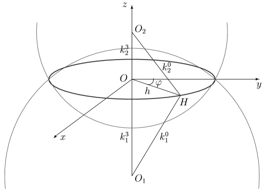
Figure 1: The interference picture in a plane $\Sigma_{t}$. Sphere $S_{a}$ with radius $k_{a}^{0}=t-t_{a}$ is centered at point $O_{a}$ with coordinates $z_{a}^{i^{\prime}}(t_{a}),i^{\prime}=1,2,3$. Angle $\varphi$ distinguishes the points of intersection $S_{1}\cap S_{2}=C(O,h)$ which constitute support of integrals (2.1) and (2.2). $k_{a}^{0}$, $k_{a}^{3}$, and $h$ are the components of the future oriented null 4-vector $k_{a}^{\alpha^{\prime}}=\Omega^{\alpha^{\prime}}{}_{\alpha}(y^{\alpha}-z_{a}^{\alpha}(t_{a}))$. Matrix $\hat{\Omega}$ determines transition to “momentarily rotating” Lorentz frame.

2.1 Local map

To find the local expressions for coordinate transformation $(y^{\alpha})\mapsto(t,t_{1},t_{2},\varphi)$, we translate the origin of the laboratory Lorentz frame at the center $O$ of the circle $C(O,h)=S_{1}\cap S_{2}$ and then rotate space axes till a new $z$-axis be directed along 3-vector ${\mathbf{q}}:={\mathbf{z}}_{1}-{\mathbf{z}}_{2}$,

$$y^{\alpha}=z_{a}^{\alpha}(t_{a})+\Omega^{\alpha}{}_{\alpha^{\prime}}(t_{1},t_{2})k_{a}^{\alpha^{\prime}}.$$ (2.4)

Here $k_{a},a=1,2$ is the future oriented null-vector with components

$$k_{a}^{0}=t-t_{a},\quad k_{a}^{1}=h\sin\varphi,\quad k_{a}^{2}=h\cos\varphi,\quad k_{a}^{3}=(-1)^{a}\frac{\rm q}{2}+\frac{(k_{2}^{0})^{2}-(k_{1}^{0})^{2}}{2{\rm q}},$$ (2.5)

which arise from analysis of triangle $O_{1}O_{2}H$ pictured in Fig. 1 (we denote ${\rm q}=|{\mathbf{q}}|$). Matrix space-time components are $\Omega_{0\mu}=\Omega_{\mu 0}=\delta_{\mu 0}$. Its space components $\Omega_{ij}$ constitute an orthogonal $3\times 3$ matrix (A.6) which determines the rotation described above (see Appendix A). It defines new orthonormal basis,

$${\mathbf{n}}_{\vartheta} = \cos\varphi_{q}\cos\vartheta_{q}{\mathbf{e}}_{1}+\sin\varphi_{q}\cos\vartheta_{q}{\mathbf{e}}_{2}-\sin\vartheta_{q}{\mathbf{e}}_{3}\,,$$

$${\mathbf{n}}_{\varphi} = -\sin\varphi_{q}{\mathbf{e}}_{1}+\cos\varphi_{q}{\mathbf{e}}_{2}\,,$$ (2.6)

$${\mathbf{n}}_{q} = \cos\varphi_{q}\sin\vartheta_{q}{\mathbf{e}}_{1}+\sin\varphi_{q}\sin\vartheta_{q}{\mathbf{e}}_{2}+\cos\vartheta_{q}{\mathbf{e}}_{3}\,,$$

which is constructed from components of the relative position 3-vector ${\mathbf{q}}$, e.g. $\cos\varphi_{q}=q^{1}/\sqrt{(q^{1})^{2}+(q^{2})^{2}}$, $\cos\vartheta_{q}=q^{3}/{\rm q}$.

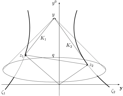
Figure 2: The past light cone with vertex at point $y\in\Sigma_{t}$ is punctured by the world lines of the 1-st particle and the 2-nd particle at points $z_{1}(t_{1})$ and $z_{2}(t_{2})$, respectively. The vector $K_{a}$ is a null vector pointing from the emission point $z_{a}(t_{a})=(t_{a},z_{a}^{i}(t_{a}))$ to a field point $y$. The relative position 4-vector $q=z_{1}-z_{2}$ is equal to difference $K_{2}-K_{1}$; its square $(q\cdot q)=-2(K_{2}\cdot K_{1})$.

To find the Jacobian of coordinate transformation (2.4), we derive its differential chart. Setting $\alpha=0$ in eq.(2.4) immediately follows $y^{0}=t$. Since $t=y^{0}$, then $\partial t/\partial y^{\alpha}=\delta_{0\alpha}$. Because $y$ and $z_{a}(t_{a})$ lie on the light cone (see Fig. 2), a change field point $y$ comes with a change in $t_{a}$. Suppose that $y$ is displaced to the new point $y+\delta y$. The new intersection of the past light cone of this vertex with the $a$-th world line is then $z_{a}(t_{a}+\delta t_{a})$. These points are still related by the equation

$$(y^{0}+\delta y^{0}-t_{a}-\delta t_{a})^{2}=\sum_{i}(y^{i}+\delta y^{i}-z_{a}^{i}(t_{a}+\delta t_{a}))^{2}.$$ (2.7)

Expanding this to the first order in $\delta y$ and $\delta t_{a}$ and using the cone equation (2.3), we obtain $K_{a,\alpha}\delta y^{\alpha}-(v_{a}\cdot K_{a})\delta t_{a}=0$ or

$$\frac{\displaystyle\partial t_{a}}{\displaystyle\partial y^{\alpha}} = -\frac{\displaystyle K_{a,\alpha}}{\displaystyle r_{a}}$$

$$= -\frac{\displaystyle\Omega_{\alpha\alpha^{\prime}}k_{a}^{\alpha^{\prime}}}{\displaystyle r_{a}}.$$

Here $K_{a}$ is $a$-th null vector pictured in figure 2 and symbol $r_{a}$ denotes the scalar product $(v_{a}\cdot K_{a})$, taken with opposite sign; noncovariant 4-velocity $v_{a}:=(1,{\rm d}z_{a}^{i}/{\rm d}t_{a})$.

For the angular variable we have

$$\frac{\displaystyle\partial\varphi}{\displaystyle\partial y^{\alpha}}=\Omega_{\alpha\alpha^{\prime}}k_{\varphi}^{\alpha^{\prime}},$$ (2.9)

where

$$k_{\varphi}^{0}=0,\quad k_{\varphi}^{1}=\frac{\displaystyle\cos\varphi}{\displaystyle h},\quad k_{\varphi}^{2}=-\frac{\displaystyle\sin\varphi}{\displaystyle h},\quad k_{\varphi}^{3}=0.$$ (2.10)

Recall that $h$ is the radius of the circle $C(O,h)=S_{1}\cap S_{2}$ pictured in Fig. 1.

Determinant of the matrix which defines this differential chart gives the inverse Jacobian: $J^{-1}={\rm q}/(r_{1}r_{2})$. The “interference” surface element,

$${\rm d}\sigma_{0}=\frac{\displaystyle r_{1}r_{2}}{\displaystyle\rm q}{\rm d}t_{1}{\rm d}t_{2}{\rm d}\varphi,$$ (2.11)

is ill defined if and only if the particles are very close to each other.

2.2 Global mapping

Setting $a=1$ in eq.(2.4) we obtain the coordinate system centered on an accelerated world line of the first particle. The flat spacetime ${\mathbb{M}}_{4}$ is a disjoint union of hyperplanes $\Sigma_{t}=\{y\in{\mathbb{M}}_{4}:y^{0}=t\}$. An interference hyperplane $\Sigma_{t}$ is a disjoint union of retarded spheres $S_{1}(O_{1},t-t_{1})$ centered at points $O_{1}\in\Sigma_{t}$ with coordinates ${\mathbf{z}}_{1}(t_{1})$. A sphere is covered by its intersections with spherical wave fronts of the second source. Each circle $S_{1}\cap S_{2}$ can be labelled by the individual time $t_{2}$ of the second particle and each point on a given circle can be labelled by its polar angle $\varphi$.

Going along the world line $\zeta_{1}$ we arrive unavoidably at the point $t_{1}^{ret}(t)$, such that the future light cone of $z_{1}[t_{1}^{ret}(t)]$ touches the 2-nd world line at point $z_{2}(t)\in\Sigma_{t}$ (see Fig. 4). Light cone of upper vertices do not intersect the second world line at all.

In context with the principle of retarded causality, $\Sigma_{t}$ is divided into two regions where outgoing waves sourced by charged particles combine in quite different manner.

• Causal, which is filled up by spheres $S_{1}$ of radii larger than or equal to $t-t_{1}^{ret}(t)$.

• Acausal, where parameter $t_{1}$ increases from $t_{1}^{ret}(t)$ to the instant of observation $t$. It is the ball bounded by sphere of radius $t-t_{1}^{ret}(t)$ centered at point ${\mathbf{z}}_{1}[t_{1}^{ret}(t)]$.

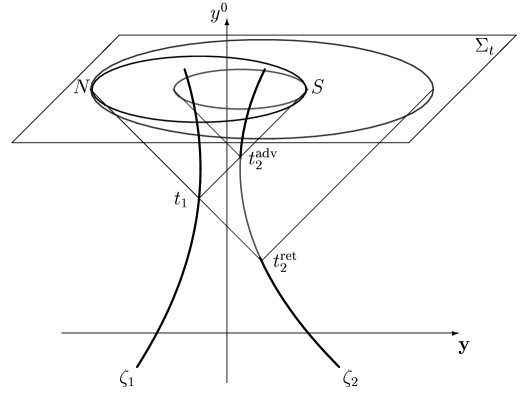
Figure 3: For a given $t_{1}$ the wave front $S_{1}$ is covered by circles $S_{1}\cap S_{2}$ if the parameter $t_{2}$ increases from $t_{2}^{\rm ret}(t_{1})$ to $t_{2}^{\rm adv}(t_{1})$. Minimal value labels the vertex of forward light cone which is punctured by $\zeta_{1}$ at $z_{1}(t_{1})$. The largest sphere $S_{2}^{\rm ret}$ touches the sphere $S_{1}$ at point $N$. World line $\zeta_{2}$ punctures the future light cone of $z_{1}(t_{1})$ at point $z_{2}(t_{2}^{\rm adv})$. Intersection of $S_{1}$ and the smallest sphere $S_{2}^{\rm adv}$ contains the only point $S$.

2.2.1 Causal region

Causal region is spanned by curvilinear coordinates (2.4) where $t_{1}$ increases from $-\infty$ to the instant $t_{1}^{ret}(t)$. To cover the sphere $S_{1}$ where $t_{1}$ is fixed we change the parameter $t_{2}$ which labels point $z_{2}(t_{2})\in\zeta_{2}$. The starting point is the solution $t_{2}^{ret}(t_{1})$ of algebraic equation $q^{0}={\rm q}$ or

$$t_{1}-t_{2}={\rm q}(t_{1},t_{2}),$$ (2.12)

where points $z_{1}(t_{1})\in\zeta_{1}$ and $z_{2}(t_{2}^{ret})\in\zeta_{2}$ are linked by a null ray. The largest sphere $S_{2}(O_{2}^{ret},t-t_{2}^{ret})$ touches a given sphere $S_{1}(O_{1},t-t_{1})$ at only point N (see Fig. 3). If parameter $t_{2}$ increases to $t_{2}^{adv}(t_{1})$ being the solution of algebraic equation $q^{0}=-{\rm q}$ or

$$t_{2}-t_{1}={\rm q}(t_{1},t_{2}),$$ (2.13)

the intersection $S_{1}\cap S_{2}^{adv}$ contains the only point S. If parameter $t_{2}$ changes from $t_{2}^{ret}(t_{1})$ to $t_{2}^{adv}(t_{1})$, the sphere $S_{1}$ is covered by circles $C(O,h)=S_{1}\cap S_{2}$.

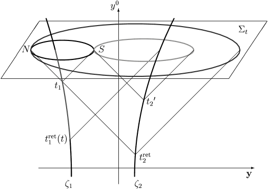
Figure 4: The instant $t_{1}^{ret}(t)$ is the solution of algebraic equation (2.13) with $t_{2}=t$. Sphere $S_{1}({\mathbf{z}}_{1}^{ret},t-t_{1}^{ret}(t))$ bounds acausal region. For a given $t_{1}\in[t_{1}^{ret}(t),t]$ the sphere $S_{1}$ with radius $t-t_{1}$ is a disjoint union of circles $S_{1}\cap S_{2}$ if parameter $t_{2}$ increases from $t_{2}^{ret}(t_{1})$ to $t_{2}^{\prime}(t,t_{1})$. The maximal value satisfies algebraic equation $k_{2}^{0}+k_{1}^{0}=|{\bf q}|$. The sphere $S_{2}{}^{\prime}$ with radius $t-t_{2}^{\prime}$ touches $S_{1}$ at point $S$. Intersection $S_{1}\cap S_{2}^{ret}$ contains the only point $N$.

2.2.2 Acausal region

Acausal region of an interference hyperplane $\Sigma_{t}$ corresponds to the fragments of the world lines which are not related to each other. (By this we mean that the radiation emitted by the first particle during the interval $[t_{1}^{ret}(t),t]$ does not come to the second one and vice versa.) Nevertheless, the outgoing waves of these portions of world lines combine in $\Sigma_{t}$ .

Acausal region is filled up by spheres $S_{1}(O_{1},t-t_{1})\in\Sigma_{t}$, where $t_{1}\in[t_{1}^{ret}(t),t]$. The sphere $S_{1}$ with fixed $t_{1}$ is the disjoint union of circles $C(O,h)=S_{1}\cap S_{2}$ if the parameter $t_{2}$ increases from $t_{2}^{ret}(t_{1})$ to $t_{2}^{\prime}(t,t_{1})$. The starting point of this interval is still the solution of eq.(2.12) while the maximal value of $t_{2}$ satisfies the algebraic equation $k_{2}^{0}+k_{1}^{0}={\rm q}$ or

$$2t-t_{1}-t_{2}={\rm q}(t_{1},t_{2}).$$ (2.14)

A given sphere $S_{1}(O_{1},t-t_{1})$ touches $S_{2}(O_{2}^{\prime},t-t_{2}^{\prime})$ at only point $S$ (see Fig. 4).

2.2.3 Surface integration

In an analogous way we construct the coordinate system centered on the world line of the second particle. If $t_{2}\in]-\infty,t_{2}^{ret}(t)]$ then $t_{1}\in[t_{1}^{ret}(t_{2}),t_{1}^{adv}(t_{2})]$; if $t_{2}\in[t_{2}^{ret}(t),t]$ then $t_{1}\in[t_{1}^{ret}(t_{2}),t_{1}^{\prime}(t,t_{2})]$, $\varphi\in[0,2\pi[$. The ends of intervals are defined implicitly by algebraic equations (2.12), (2.13), and (2.14).

The surface integration (2.1) and (2.2) can be performed via the coordinate system centered on a world line either of the first particle,

$$\left[\int\limits_{-\infty}^{t_{1}^{ret}(t)}{\rm d}t_{1}\int\limits_{t_{2}^{ret}(t_{1})}^{t_{2}^{adv}(t_{1})}{\rm d}t_{2}+\int\limits_{t_{1}^{ret}(t)}^{t}{\rm d}t_{1}\int\limits_{t_{2}^{ret}(t_{1})}^{t_{2}^{\prime}(t,t_{1})}{\rm d}t_{2}\right]\int_{0}^{2\pi}{\rm d}\varphi\frac{r_{1}r_{2}}{\rm q}\,,$$ (2.15)

or of the second particle,

$$\left[\int\limits_{-\infty}^{t_{2}^{ret}(t)}{\rm d}t_{2}\int\limits_{t_{1}^{ret}(t_{2})}^{t_{1}^{adv}(t_{2})}{\rm d}t_{1}+\int\limits_{t_{2}^{ret}(t)}^{t}{\rm d}t_{2}\int\limits_{t_{1}^{ret}(t_{2})}^{t_{1}^{\prime}(t,t_{2})}{\rm d}t_{1}\right]\int_{0}^{2\pi}{\rm d}\varphi\frac{r_{1}r_{2}}{\rm q}\,.$$ (2.16)

To calculate the flows (2.1) of the mixed electromagnetic field energy and momentum which flow across the hyperplane $\Sigma_{t}$, we should integrate the Maxwell energy-momentum tensor density (1.5) over angular variable $\varphi$ and over time variables $t_{1}$ and $t_{2}$.

3 Angular integration of energy-momentum and angular momentum tensor densities

In this Section we trace a series of stages in integration of the mixed Maxwell energy-momentum tensor density over $\varphi$. In Appendix A we derive some useful expressions.

In terms of Minkowski coordinates $(y^{\alpha})$ the electromagnetic field generated by $a$-th particle is given by

$${\hat{f}}_{(a)}=\frac{e_{a}}{{\sf r}_{a}^{2}}u_{a}\wedge{\sf k}_{a}+\frac{e_{a}}{{\sf r}_{a}}\left[a_{a}\wedge{\sf k}_{a}+({\sf k}_{a}\cdot a_{a})u_{a}\wedge{\sf k}_{a}\right],$$ (3.1)

where symbol $\wedge$ denotes the wedge product. We use sans-serif symbols for the retarded distance,

$${\sf r}_{a}=-\eta_{\alpha\beta}\left(y^{\alpha}-z_{a}^{\alpha}(s_{a})\right)u_{a}^{\beta}(s_{a}),$$ (3.2)

and for the null vector $K_{a}=y-z_{a}(s_{a})$ rescaled by a factor ${\sf r}_{a}^{-1}$,

$${\sf k}_{a}^{\alpha}=\frac{1}{{\sf r}_{a}}\left(y^{\alpha}-z_{a}^{\alpha}(s_{a})\right).$$ (3.3)

To express field strengths in terms of curvilinear coordinates $(t,t_{1},t_{2},\varphi)$, it is advantageous to replace the retarded proper time $s_{a}(y)$ by evolution parameter $t_{a}$. The components of particles’ 4-velocities $u_{a}$ and 4-accelerations $a_{a}$, $a=1,2$, become [2]

$$u_{a}^{\mu}=\gamma_{a}v_{a}^{\mu}(t_{a}),\qquad a_{a}^{\mu}=\gamma_{a}^{4}(v_{a}\cdot{\dot{v}}_{a})v_{a}^{\mu}+\gamma_{a}^{2}{\dot{v}}_{a}^{\mu},$$ (3.4)

where 4-vectors $v_{a}^{\mu}=(1,v_{a}^{i}(t_{a}))$, ${\dot{v}}_{a}^{\mu}=(0,{\dot{v}}_{a}^{i}(t_{a}))$ and factor $\gamma_{a}:=[1-{\mathbf{v}}_{a}^{2}]^{-1/2}$. Substituting these into eq.(3.1) and using the relation ${\sf k}_{a}^{\mu}=K_{a}^{\mu}/{\sf r}_{a}$ yields

$${\hat{f}}_{(a)}=e_{a}\left(\frac{v_{a}\wedge K_{a}}{r_{a}^{3}}c_{a}+\frac{{\dot{v}}_{a}\wedge K_{a}}{r_{a}^{2}}\right),$$ (3.5)

where

$$r_{a}=K_{a}^{0}-({\bf K}_{a}{\bf v}_{a}),\qquad c_{a}=\gamma_{a}^{-2}+({\bf K}_{a}{\bf\dot{v}}_{a}).$$ (3.6)

Note that $r_{a}$ is the retarded distance (3.2) rescaled by a factor $\gamma_{a}$, i.e. $r_{a}=\gamma_{a}^{-1}{\sf r}_{a}$. The separation vector $K_{a}$ has the form ${\hat{\Omega}}k_{a}$, where components of null vector $k_{a}$ are given by eqs.(2.5) and matrix $\hat{\Omega}$ determines the transition to momentarily comoving Lorentz frame associated with basis (2.1).

It is straightforward to substitute the components of electromagnetic fields (3.5) in terms of “interference” coordinates $(t,t_{1},t_{2},\varphi)$ into integrands of expressions (2.1) and (2.2) to calculate the interference part of radiated energy-momentum and angular momentum, respectively. Integration of the mixed stress-energy tensor over angular variable is the key to the problem. All $\varphi$-dependent terms are concentrated in the following constructions:

$${\cal D}^{a} = \frac{1}{2\pi}\int\limits_{0}^{2\pi}{\rm d}\varphi\frac{a}{{\rm q}r_{1}r_{2}},\qquad{\cal B}^{a}=\frac{1}{2\pi}\int\limits_{0}^{2\pi}{\rm d}\varphi\frac{ac_{2}}{{\rm q}r_{1}(r_{2})^{2}},$$ (3.7)

$${\cal C}^{a} = \frac{1}{2\pi}\int\limits_{0}^{2\pi}{\rm d}\varphi\frac{ac_{1}}{{\rm q}(r_{1})^{2}r_{2}},\qquad{\cal A}^{a}=\frac{1}{2\pi}\int\limits_{0}^{2\pi}{\rm d}\varphi\frac{ac_{1}c_{2}}{{\rm q}(r_{1})^{2}(r_{2})^{2}}.$$

They are labeled according to their dependence on the combination of components of the separation vectors $K_{1}$ and $K_{2}$: factor $a$ is replaced by $K_{1}^{\mu}K_{2}^{\nu},K_{1}^{\mu},K_{2}^{\nu}$, or $1$ for ${\cal D}^{\mu\nu}_{12}$, ${\cal D}^{\mu}_{1}$, ${\cal D}^{\nu}_{2}$ or ${\cal D}^{0}$, respectively. (The others ${\cal B}^{a},{\cal C}^{a}$, and ${\cal A}^{a}$ are marked analogously.)

The mixed part of the stress-energy tensor (1.5) is symmetric in indices $1$ and $2$. Substituting (3.5) into the first term of this expression and using the identities $K_{2}-K_{1}=q$ and $(K_{2}\cdot K_{1})=-1/2(q\cdot q)$ yields

$$\frac{1}{4\pi}\int\limits_{0}^{2\pi}{\rm d}\varphi\!\!\!\!\!\!\!\!\!\!\!\! Jf^{\mu\alpha}_{(1)}f^{\nu}_{(2)\alpha}=\frac{e_{1}e_{2}}{2}\left\{{\cal T}^{\mu\nu}_{12}\left(\frac{\partial^{2}\sigma}{\partial t_{1}\partial t_{2}}\right)+{\cal T}^{\mu}_{1}\left(v_{2}^{\nu}\frac{\partial\sigma}{\partial t_{1}}\right)+{\cal T}^{\nu}_{2}\left(v_{1}^{\mu}\frac{\partial\sigma}{\partial t_{2}}\right)+{\cal T}^{0}(v_{1}^{\mu}v_{2}^{\nu}\sigma)\right.$$

$$- \left.{\cal C}_{1}^{\mu}v_{2}^{\nu}\frac{\partial^{2}\sigma}{\partial t_{1}\partial t_{2}}-{\cal D}_{1}^{\mu}v_{2}^{\nu}\frac{\partial^{3}\sigma}{\partial t_{1}^{2}\partial t_{2}}-{\cal B}_{2}^{\nu}v_{1}^{\mu}\frac{\partial^{2}\sigma}{\partial t_{1}\partial t_{2}}-{\cal D}_{2}^{\nu}v_{1}^{\mu}\frac{\partial^{3}\sigma}{\partial t_{1}\partial t_{2}^{2}}\right.$$

$$- \left.{\cal B}^{0}v_{1}^{\mu}v_{2}^{\nu}\frac{\partial\sigma}{\partial t_{1}}-{\cal C}^{0}v_{1}^{\mu}v_{2}^{\nu}\frac{\partial\sigma}{\partial t_{2}}-{\cal D}^{0}\left({\dot{v}}_{1}^{\mu}v_{2}^{\nu}\frac{\partial\sigma}{\partial t_{2}}+v_{1}^{\mu}{\dot{v}}_{2}^{\nu}\frac{\partial\sigma}{\partial t_{1}}+v_{1}^{\mu}v_{2}^{\nu}\frac{\partial^{2}\sigma}{\partial t_{1}\partial t_{2}}\right)\right\},$$

after addition of similar terms and integration over $\varphi$. World function $\sigma(t_{1},t_{2})$ of two spacelike related points, $z_{1}(t_{1})\in\zeta_{1}$ and $z_{2}(t_{2})\in\zeta_{2}$, is equal to one-half of the square of vector $q=z_{1}-z_{2}$, taken with opposite sign,

$$\sigma(t_{1},t_{2})=-1/2(q\cdot q).$$ (3.9)

Each second order differential operator,

$${\hat{\cal T}}^{a}={\cal D}^{a}\frac{\partial^{2}}{\partial t_{1}\partial t_{2}}+{\cal B}^{a}\frac{\partial}{\partial t_{1}}+{\cal C}^{a}\frac{\partial}{\partial t_{2}}+{\cal A}^{a},$$ (3.10)

has been labeled according to dependence of coefficients (3.7) on the combination of vectors $K_{1}$ and $K_{2}$.

For the convolution $f^{\alpha\beta}_{(1)}f^{(2)}_{\alpha\beta}$, we obtain

$$\frac{1}{4\pi}\int\limits_{0}^{2\pi}{\rm d}\varphi Jf^{\alpha\beta}_{(1)}f^{(2)}_{\alpha\beta}=e_{1}e_{2}{\cal T}^{0}(\lambda),$$ (3.11)

where function

$$\lambda=\sigma\frac{\partial^{2}\sigma}{\partial t_{1}\partial t_{2}}-\frac{\partial\sigma}{\partial t_{1}}\frac{\partial\sigma}{\partial t_{2}}$$ (3.12)

depends on two-point function (3.9) and its derivatives in time variables.

To distinguish the partial derivatives in time variables, we rewrite the operator (3.10) as the sum of the second-order differential operator,

$${\hat{\Pi}}^{a}=\frac{\partial^{2}}{\partial t_{1}\partial t_{2}}{\cal D}^{a}+\frac{\partial}{\partial t_{1}}\left({\cal B}^{a}-\frac{\partial{\cal D}^{a}}{\partial t_{2}}\right)+\frac{\partial}{\partial t_{2}}\left({\cal C}^{a}-\frac{\partial{\cal D}^{a}}{\partial t_{1}}\right),$$ (3.13)

and the “tail”,

$$\pi^{a}=\frac{\partial^{2}{\cal D}^{a}}{\partial t_{1}\partial t_{2}}-\frac{\partial{\cal B}^{a}}{\partial t_{1}}-\frac{\partial{\cal C}^{a}}{\partial t_{2}}+{\cal A}^{a}.$$ (3.14)

For a smooth function $f(t_{1},t_{2})$ we have

$${\hat{\cal T}}^{a}(f)={\hat{\Pi}}^{a}(f)+f\pi^{a}.$$ (3.15)

Cumbersome calculations which are presented in Appendix A give the relations

$$\pi^{0} = 0,$$ (3.16)

$$\pi_{1}^{\mu} = v_{1}^{\mu}\left({\cal B}^{0}-\frac{\partial{\cal D}^{0}}{\partial t_{2}}\right),\qquad\pi_{2}^{\nu}=v_{2}^{\nu}\left({\cal C}^{0}-\frac{\partial{\cal D}^{0}}{\partial t_{1}}\right),$$

$$\pi_{12}^{\mu\nu} = v_{1}^{\mu}\left({\cal B}_{2}^{\nu}-\frac{\partial{\cal D}_{2}^{\nu}}{\partial t_{2}}\right)+v_{2}^{\nu}\left({\cal C}_{1}^{\mu}-\frac{\partial{\cal D}_{1}^{\mu}}{\partial t_{1}}\right)-v_{1}^{\mu}v_{2}^{\nu}{\cal D}^{0},$$

which allow us to rewrite the sum of integrals (3) and (3.11) in terms of differential operators ${\hat{\Pi}}^{a}$ and partial derivatives in $t_{1}$ and $t_{2}$,

$${\cal P}^{\mu\nu}_{12} = \frac{1}{4\pi}\int_{0}^{2\pi}d\varphi J\left(f_{(1)}^{\mu\alpha}f_{(2)\alpha}^{\nu}-\frac{\eta^{\mu\nu}}{4}f_{(1)}^{\alpha\beta}f_{\alpha\beta}^{(2)}\right)$$

$$= \frac{e_{1}e_{2}}{2}\left\{{\hat{\Pi}}^{\mu\nu}_{12}\left(\frac{\partial^{2}\sigma}{\partial t_{1}\partial t_{2}}\right)+{\hat{\Pi}}^{\mu}_{1}\left(v_{2}^{\nu}\frac{\partial\sigma}{\partial t_{1}}\right)+{\hat{\Pi}}^{\nu}_{2}\left(v_{1}^{\mu}\frac{\partial\sigma}{\partial t_{2}}\right)+{\hat{\Pi}}^{0}(v_{1}^{\mu}v_{2}^{\nu}\sigma)\right.$$

$$- \left.\frac{\partial}{\partial t_{1}}\left({\cal D}_{1}^{\mu}v_{2}^{\nu}\frac{\partial^{2}\sigma}{\partial t_{1}\partial t_{2}}\right)-\frac{\partial}{\partial t_{2}}\left({\cal D}_{2}^{\nu}v_{1}^{\mu}\frac{\partial^{2}\sigma}{\partial t_{1}\partial t_{2}}\right)\right.$$

$$- \left.\frac{\partial}{\partial t_{1}}\left({\cal D}^{0}v_{1}^{\mu}v_{2}^{\nu}\frac{\partial\sigma}{\partial t_{2}}\right)-\frac{\partial}{\partial t_{2}}\left({\cal D}^{0}v_{1}^{\mu}v_{2}^{\nu}\frac{\partial\sigma}{\partial t_{1}}\right)-\frac{1}{2}\eta^{\mu\nu}{\hat{\Pi}}^{0}(\lambda)\right\}.$$

We denote ${\cal P}^{\mu\nu}_{21}$ the integral over $\varphi$ of the remaining terms involved in tensor (1.5). It can be obtained by interchanging of indices 1 and 2.

Setting $\mu=0$ and $\nu=i$ in eq.(3), we obtain the first term of the mixed space-time components of the stress-energy tensor (1.5). We add the term where indices $1$ and $2$ are interchanged. Since zeroth components $k_{1}^{0}$ and $k_{2}^{0}$ of the separation four-vectors $K_{1}$ and $K_{2}$ do not depend on $\varphi$, the final expression get simplified,

$${\cal P}^{i}_{\rm int} = {\cal P}^{0i}_{12}+{\cal P}^{0i}_{21}$$

$$= \frac{e_{1}e_{2}}{2}\left[{\hat{\Pi}}_{2}^{i}\left(\frac{\partial\lambda_{1}}{\partial t_{2}}\right)+{\hat{\Pi}}_{1}^{i}\left(\frac{\partial\lambda_{2}}{\partial t_{1}}\right)+{\hat{\Pi}}^{0}\left(v_{2}^{i}\lambda_{1}+v_{1}^{i}\lambda_{2}\right)\right.$$

$$- \left.\frac{\partial}{\partial t_{1}}\left(v_{2}^{i}\frac{\partial\lambda_{1}}{\partial t_{2}}{\cal D}^{0}\right)-\frac{\partial}{\partial t_{2}}\left(v_{1}^{i}\frac{\partial\lambda_{2}}{\partial t_{1}}{\cal D}^{0}\right)\right],$$

where

$$\lambda_{1}=k_{1}^{0}\frac{\partial\sigma}{\partial t_{1}}+\sigma,\qquad\lambda_{2}=k_{2}^{0}\frac{\partial\sigma}{\partial t_{2}}+\sigma.$$ (3.19)

Similarly we derive zeroth component ${\cal P}^{0}_{\rm int}$. Setting $\mu=0$ and $\nu=0$ in eq.(3), we obtain the first one-half of desired expression. The second one, ${\cal P}^{00}_{21}$, can be derived via interchanging indices $1$ and $2$. The integral of energy density $T^{00}_{\rm int}$ over the angular variable has the form

$${\cal P}^{0}_{\rm int} = {\cal P}^{00}_{12}+{\cal P}^{00}_{21}$$

$$= \frac{e_{1}e_{2}}{2}{\hat{\Pi}}^{0}\left(\Sigma\frac{\partial^{2}\Sigma}{\partial t_{1}\partial t_{2}}-\frac{\partial\Sigma}{\partial t_{1}}\frac{\partial\Sigma}{\partial t_{2}}\right),$$

where three-point function,

$$\Sigma(t,t_{1},t_{2})=2k_{1}^{0}k_{2}^{0}+\sigma(t_{1},t_{2}),$$ (3.21)

depends on particles’ positions referred to the moments $t_{1}$ and $t_{2}$ before observation instant $t$ as well as on $t$ itself.

We now turn to the integration of the angular momentum tensor density (2.2) carried by the electromagnetic field due to two pointlike charges. We present the torque $m_{\rm int}^{\mu\nu}=y^{\mu}T_{\rm int}^{0\nu}-y^{\nu}T_{\rm int}^{0\mu}$ in the following form:

$$m_{\rm int}^{\mu\nu}=m_{12}^{\mu\nu}+m_{21}^{\mu\nu}-m_{12}^{\nu\mu}-m_{21}^{\nu\mu},$$ (3.22)

where

$$m_{12}^{\mu\nu}=\left(z_{1}^{\mu}+K_{1}^{\mu}\right)\frac{1}{4\pi}\left[f_{(1)}^{0\lambda}f_{(2)\lambda}^{\nu}-\frac{1}{4}\eta^{0\nu}f_{(1)}^{\alpha\beta}f^{(2)}_{\alpha\beta}\right].$$ (3.23)

It is straightforward to substitute the fields (3.5) into this expression to calculate the first term of expression (3.22). The others can be obtained by interchanging of the pair of indices $(1,2)$ and $(\mu,\nu)$.

Having integrated expression $Jm_{12}^{\mu\nu}$ over $\varphi$ we obtain

$${\cal M}_{12}^{\mu\nu} = \frac{e_{1}e_{2}}{2}\left\{{\hat{\cal T}}_{12}^{\mu\nu}\left(\frac{\partial\lambda_{1}}{\partial t_{2}}\right)+{\hat{\cal T}}_{1}^{\mu}\left(v_{2}^{\nu}\lambda_{1}\right)-v_{2}^{\nu}\frac{\partial\lambda_{1}}{\partial t_{2}}{\cal C}_{1}^{\mu}-v_{2}^{\nu}\frac{\partial^{2}\lambda_{1}}{\partial t_{1}\partial t_{2}}{\cal D}_{1}^{\mu}\right.$$ (3.24)

$$+ \left.{\hat{\cal T}}_{2}^{\nu}\left(z_{1}^{\mu}\frac{\partial\lambda_{1}}{\partial t_{2}}\right)-v_{1}^{\mu}\frac{\partial\lambda_{1}}{\partial t_{2}}{\cal B}_{2}^{\nu}-v_{1}^{\mu}\frac{\partial^{2}\lambda_{1}}{\partial t_{2}^{2}}{\cal D}_{2}^{\nu}+{\hat{\cal T}}^{0}\left(z_{1}^{\mu}v_{2}^{\nu}\lambda_{1}\right)-v_{1}^{\mu}v_{2}^{\nu}\lambda_{1}{\cal B}^{0}\right.$$

$$- \left.v_{1}^{\mu}\left({\dot{v}}_{2}^{\nu}\lambda_{1}+v_{2}^{\nu}\frac{\partial\lambda_{1}}{\partial t_{2}}{\cal D}^{0}\right)-z_{1}^{\mu}v_{2}^{\nu}\frac{\partial\lambda_{1}}{\partial t_{2}}{\cal C}^{0}-z_{1}^{\mu}v_{2}^{\nu}\frac{\partial^{2}\lambda_{1}}{\partial t_{1}\partial t_{2}}{\cal D}^{0}\right.$$

$$- \left.\frac{\eta^{0\nu}}{2}\left[{\hat{\cal T}}_{1}^{\mu}\left(\lambda\right)+{\hat{\cal T}}^{0}\left(z_{1}^{\mu}\lambda\right)-v_{1}^{\mu}\lambda{\cal B}^{0}-v_{1}^{\mu}\frac{\partial\lambda}{\partial t_{2}}{\cal D}^{0}\right]\right\},$$

where functions $\lambda$ and $\lambda_{a}$ are given by eqs.(3.12) and (3.19), respectively.

Usage of the equalities in eq.(3.16) derived in Appendix A allows us to rewrite the integrand (3.24) as follows:

$${\cal M}_{12}^{\mu\nu} = \frac{e_{1}e_{2}}{2}\left\{{\hat{\Pi}}_{12}^{\mu\nu}\left(\frac{\partial\lambda_{1}}{\partial t_{2}}\right)+{\hat{\Pi}}_{1}^{\mu}\left(v_{2}^{\nu}\lambda_{1}\right)-\frac{\partial}{\partial t_{1}}\left(v_{2}^{\nu}\frac{\partial\lambda_{1}}{\partial t_{2}}{\cal D}_{1}^{\mu}\right)\right.$$

$$+ \left.{\hat{\Pi}}_{2}^{\nu}\left(z_{1}^{\mu}\frac{\partial\lambda_{1}}{\partial t_{2}}\right)-\frac{\partial}{\partial t_{2}}\left(v_{1}^{\mu}\frac{\partial\lambda_{1}}{\partial t_{2}}{\cal D}_{2}^{\nu}\right)\right.$$

$$+ \left.{\hat{\Pi}}^{0}\left(z_{1}^{\mu}v_{2}^{\nu}\lambda_{1}\right)-\frac{\partial}{\partial t_{1}}\left(z_{1}^{\mu}v_{2}^{\nu}\frac{\partial\lambda_{1}}{\partial t_{2}}{\cal D}^{0}\right)-\frac{\partial}{\partial t_{2}}\left(v_{1}^{\mu}v_{2}^{\nu}\lambda_{1}{\cal D}^{0}\right)\right.$$

$$- \left.\frac{\eta^{0\nu}}{2}\left[{\hat{\Pi}}_{1}^{\mu}\left(\lambda\right)+{\hat{\Pi}}^{0}\left(z_{1}^{\mu}\lambda\right)-\frac{\partial}{\partial t_{2}}\left(v_{1}^{\mu}\lambda{\cal D}^{0}\right)\right]\right\}.$$

The other terms of mixed angular momentum,

$${\cal M}_{\rm int}^{\mu\nu}={\cal M}_{12}^{\mu\nu}+{\cal M}_{21}^{\mu\nu}-{\cal M}_{12}^{\nu\mu}-{\cal M}_{21}^{\nu\mu},$$ (3.26)

can be obtained via interchanging of indices $(1,2)$ and $(\mu,\nu)$.

We see that the integration of the mixed stress-energy tensor (1.5) over $\varphi$ yields the combinations of partial derivatives in time variables. In the next Section we classify them and reveal the long-range terms which contribute into radiated energy-momentum.

4 Radiative parts of mixed energy-momentum and angular momentum

In previous Section we integrate the mixed part of the stress-energy tensor and its torque over polar angle. Resulted expressions describe contributions to electromagnetic field’s energy-momentum and angular momentum due to interference of spherical wave fronts of charges $e_{1}$ and $e_{2}$ placed at fixed points $z_{1}(t_{1})\in\zeta_{1}$ and $z_{2}(t_{2})\in\zeta_{2}$, respectively. The crucial issue is that the integrals (3), (3) and (3.26) have the remarkable property of being the sum of partial derivatives in time variables. This circumstance allows us to calculate how much electromagnetic field’s energy-momentum and angular momentum flow across a hyperplane $\Sigma_{t}$.

It is natural to integrate the expression being the time derivative with respect to $t_{2}$ according to the rule (2.15),

$${\cal G}_{2} = \left[\int\limits_{-\infty}^{t_{1}^{ret}(t)}{\rm d}t_{1}\int\limits_{t_{2}^{ret}(t_{1})}^{t_{2}^{adv}(t_{1})}{\rm d}t_{2}+\int\limits_{t_{1}^{ret}(t)}^{t}{\rm d}t_{1}\int\limits_{t_{2}^{ret}(t_{1})}^{t_{2}^{\prime}(t,t_{1})}{\rm d}t_{2}\right]\frac{\partial G_{2}(t_{1},t_{2})}{\partial t_{2}}$$

$$= \int\limits_{-\infty}^{t_{1}^{ret}(t)}{\rm d}t_{1}G_{2}[t_{1},t_{2}^{adv}(t_{1})]-\int\limits_{-\infty}^{t}{\rm d}t_{1}G_{2}[t_{1},t_{2}^{ret}(t_{1})]+\int\limits_{t_{1}^{ret}(t)}^{t}{\rm d}t_{1}G_{2}[t_{1},t_{2}^{\prime}(t,t_{1})].$$

Having applied the rule (2.16) to the expression of type $\partial G_{1}/\partial t_{1}$, we obtain

$${\cal G}_{1} = \left[\int\limits_{-\infty}^{t_{2}^{ret}(t)}{\rm d}t_{2}\int\limits_{t_{1}^{ret}(t_{2})}^{t_{1}^{adv}(t_{2})}{\rm d}t_{1}+\int\limits_{t_{2}^{ret}(t)}^{t}{\rm d}t_{2}\int\limits_{t_{1}^{ret}(t_{2})}^{t_{1}^{\prime}(t,t_{2})}{\rm d}t_{1}\right]\frac{\partial G_{1}(t_{1},t_{2})}{\partial t_{1}}$$

$$= \int\limits_{-\infty}^{t_{2}^{ret}(t)}{\rm d}t_{2}G_{1}[t_{1}^{adv}(t_{2}),t_{2}]-\int\limits_{-\infty}^{t}{\rm d}t_{2}G_{1}[t_{1}^{ret}(t_{2}),t_{2}]+\int\limits_{t_{2}^{ret}(t)}^{t}{\rm d}t_{2}G_{1}[t_{1}^{\prime}(t,t_{2}),t_{2}].$$

The end points are valuable only in the integration procedure. They are solutions of algebraic equations (2.12), (2.13) and (2.14). The retarded instants $t_{a}^{ret}(t_{b})$ and advanced ones $t_{b}^{adv}(t_{a})$ label the points $N$ and $S$ in which fronts of outgoing electromagnetic waves produced by charges touch each other (see Fig. 3). All the moments are before the observation instant $t$, so that the retarded causality is not violated.

It is worth noting that the functions $t_{1}^{ret}(t_{2})$ and $t_{2}^{adv}(t_{1})$ are inverted to each other as well as the pair of functions $t_{1}^{adv}(t_{2})$ and $t_{2}^{ret}(t_{1})$. For a fixed laboratory time $t$ the functions $t_{1}^{\prime}(t,t_{2})$ and $t_{2}^{\prime}(t,t_{1})$ are inverses too. These circumstances allow us to change the variables $t_{a}\mapsto t_{a}^{ret}(t_{b})$ in the “advanced” integrals in eqs.(4) and (4). Further we couple them with their “retarded” counterparts. Since

$$\frac{{\rm d}t_{1}^{ret}(t_{2})}{{\rm d}t_{2}}=\frac{1-({\mathbf{v}}_{1}{\mathbf{n}}_{\rm q})}{1-({\mathbf{v}}_{2}{\mathbf{n}}_{\rm q})},\qquad\frac{{\rm d}t_{2}^{ret}(t_{1})}{{\rm d}t_{1}}=\frac{1+({\mathbf{v}}_{2}{\mathbf{n}}_{\rm q})}{1+({\mathbf{v}}_{1}{\mathbf{n}}_{\rm q})},$$ (4.3)

we obtain

$${\cal G}_{2}+{\cal G}_{1} = \int\limits_{-\infty}^{t}{\rm d}t_{1}\left[\frac{1-({\mathbf{v}}_{1}{\mathbf{n}}_{\rm q})}{1-({\mathbf{v}}_{2}{\mathbf{n}}_{\rm q})}G_{1}-G_{2}\right]_{t_{2}=t_{2}^{ret}(t_{1})}$$

$$+ \int\limits_{-\infty}^{t}{\rm d}t_{2}\left[-G_{1}+\frac{1+({\mathbf{v}}_{2}{\mathbf{n}}_{\rm q})}{1+({\mathbf{v}}_{1}{\mathbf{n}}_{\rm q})}G_{2}\right]_{t_{1}=t_{1}^{ret}(t_{2})}$$

$$+ \int\limits_{t_{2}^{ret}(t)}^{t}{\rm d}t_{2}\left[G_{1}+\frac{1-({\mathbf{v}}_{2}{\mathbf{n}}_{\rm q})}{1+({\mathbf{v}}_{1}{\mathbf{n}}_{\rm q})}G_{2}\right]_{t_{1}=t_{1}^{\prime}(t,t_{2})}.$$

The unit vector ${\mathbf{n}}_{q}={\mathbf{q}}/{\rm q}$ is the third vector of orthonormal triad (2.1). The last integral is due to interference of outgoing electromagnetic waves radiated out by the particles within the acausal region (see Fig. 4). We take into account that

$$\frac{{\rm d}t_{2}^{\prime}(t,t_{1})}{{\rm d}t_{1}}=-\frac{1+({\mathbf{v}}_{1}{\mathbf{n}}_{\rm q})}{1-({\mathbf{v}}_{2}{\mathbf{n}}_{\rm q})}.$$ (4.5)

Of course, one can change the variables $t_{b}\mapsto t_{b}^{adv}(t_{a})$ in the “retarded” integrals in eqs.(4) and (4) and add them to their “advanced” counterparts,

$${\cal G}_{2}+{\cal G}_{1} = \int\limits_{-\infty}^{t_{2}^{ret}(t)}{\rm d}t_{2}\left[G_{1}-\frac{1-({\mathbf{v}}_{2}{\mathbf{n}}_{\rm q})}{1-({\mathbf{v}}_{1}{\mathbf{n}}_{\rm q})}G_{2}\right]^{t_{1}=t_{1}^{adv}(t_{2})}$$

$$+ \int\limits_{-\infty}^{t_{1}^{ret}(t)}{\rm d}t_{1}\left[-\frac{1+({\mathbf{v}}_{1}{\mathbf{n}}_{\rm q})}{1+({\mathbf{v}}_{2}{\mathbf{n}}_{\rm q})}G_{1}+G_{2}\right]^{t_{2}=t_{2}^{adv}(t_{1})}$$

$$+ \int\limits_{t_{1}^{ret}(t)}^{t}{\rm d}t_{1}\left[\frac{1+({\mathbf{v}}_{1}{\mathbf{n}}_{\rm q})}{1-({\mathbf{v}}_{2}{\mathbf{n}}_{\rm q})}G_{1}+G_{2}\right]^{t_{2}=t_{2}^{\prime}(t,t_{1})}.$$

A combination of the “retarded” and the “advanced” terms is valuable too.

Integral of a mixed double derivative can be written in the form either

$${\cal I}_{1} = \left[\int\limits_{-\infty}^{t_{2}^{ret}(t)}{\rm d}t_{2}\int\limits_{t_{1}^{ret}(t_{2})}^{t_{1}^{adv}(t_{2})}{\rm d}t_{1}+\int\limits_{t_{2}^{ret}(t)}^{t}{\rm d}t_{2}\int\limits_{t_{1}^{ret}(t_{2})}^{t_{1}^{\prime}(t,t_{2})}{\rm d}t_{1}\right]\frac{\partial}{\partial t_{1}}\left[\frac{\partial G(t_{1},t_{2})}{\partial t_{2}}\right]$$

$$= \int\limits_{-\infty}^{t_{2}^{ret}(t)}{\rm d}t_{2}\left[\frac{\partial G(t_{1},t_{2})}{\partial t_{2}}\right]^{t_{1}=t_{1}^{adv}(t_{2})}-\int\limits_{-\infty}^{t}{\rm d}t_{2}\left[\frac{\partial G(t_{1},t_{2})}{\partial t_{2}}\right]_{t_{1}=t_{1}^{ret}(t_{2})}$$

$$+ \int\limits_{t_{2}^{ret}(t)}^{t}{\rm d}t_{2}\left[\frac{\partial G(t_{1},t_{2})}{\partial t_{2}}\right]^{t_{1}=t_{1}^{\prime}(t,t_{2})},$$

or

$${\cal I}_{2} = \left[\int\limits_{-\infty}^{t_{1}^{ret}(t)}{\rm d}t_{1}\int\limits_{t_{2}^{ret}(t_{1})}^{t_{2}^{adv}(t_{1})}{\rm d}t_{2}+\int\limits_{t_{1}^{ret}(t)}^{t}{\rm d}t_{1}\int\limits_{t_{2}^{ret}(t_{1})}^{t_{2}^{\prime}(t,t_{1})}{\rm d}t_{2}\right]\frac{\partial}{\partial t_{2}}\left[\frac{\partial G(t_{1},t_{2})}{\partial t_{1}}\right]$$

$$= \int\limits_{-\infty}^{t_{1}^{ret}(t)}{\rm d}t_{1}\left[\frac{\partial G(t_{1},t_{2})}{\partial t_{1}}\right]^{t_{2}=t_{2}^{adv}(t_{1})}-\int\limits_{-\infty}^{t}{\rm d}t_{1}\left[\frac{\partial G(t_{1},t_{2})}{\partial t_{1}}\right]_{t_{2}=t_{2}^{ret}(t_{1})}$$

$$+ \int\limits_{t_{1}^{ret}(t)}^{t}{\rm d}t_{1}\left[\frac{\partial G(t_{1},t_{2})}{\partial t_{1}}\right]^{t_{2}=t_{2}^{\prime}(t,t_{1})}.$$

The question is what expression should be used.

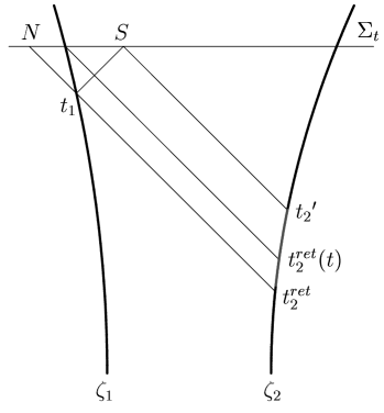
Figure 5: Function $G[t_{1},t_{2}^{ret}(t_{1})]$ is associated with the interference of wave fronts $S_{1}(O_{1},t-t_{1})$ and $S_{2}(O_{2}^{ret},t-t_{2}^{ret})$ at point $N\in\Sigma_{t}$. Function $G[t_{1},t_{2}^{\prime}(t,t_{1})]$ is connected with the combination of wave fronts $S_{1}(O_{1},t-t_{1})$ and $S_{2}(O_{2}^{\prime},t-t_{2}^{\prime})$ at point $S\in\Sigma_{t}$. If $t_{1}\to t$, both the point $N$ and the point $S$ tend to $z_{1}(t)=\zeta_{1}\cap\Sigma_{t}$. If $\lim\limits_{t_{1}\to t}G[t_{1},t_{2}^{ret}(t_{1})]=\lim\limits_{t_{1}\to t}G[t_{1},t_{2}^{\prime}(t,t_{1})]$ the value of integral of mixed derivative $\partial^{2}G/\partial t_{1}\partial t_{2}$ over time variables does not depend on the order of integration.

To compare ${\cal I}_{1}$ and ${\cal I}_{2}$ we change the variables in the “advanced” integrals and subtract (4) and (4). We arrive at the integrals being functions of the end points only,

$${\cal I}_{1}-{\cal I}_{2} = \left.\phantom{\frac{1}{1}}\!\!\!\!G[t_{1},t_{2}^{ret}(t_{1})]\right|_{t_{1}\to-\infty}^{t_{1}\to t}-\left.\phantom{\frac{1}{1}}\!\!\!\!G[t_{1}^{ret}(t_{2}),t_{2}]\right|_{t_{2}\to-\infty}^{t_{2}\to t}$$ (4.9)

$$+ \left\{\begin{array}[]{cc}{\rm either}&\left.\phantom{\frac{\displaystyle 1}{\displaystyle 1}}\!\!\!\!G[t_{1}^{\prime}(t,t_{2}),t_{2}]\right|_{t_{2}\to t_{2}^{ret}(t)}^{t_{2}\to t}\\[10.00002pt] {\rm or}&-\left.\phantom{\frac{\displaystyle 1}{\displaystyle 1}}\!\!\!\!G[t_{1},t_{2}^{\prime}(t,t_{1})]\right|_{t_{1}\to t_{1}^{ret}(t)}^{t_{1}\to t}\end{array}\right..$$ (4.12)

It vanishes if and only if (i) limiting values of $G$ (that evaluated at the remote past) cancel each other, and (ii) function $G$ is smooth at points at which the world lines puncture $\Sigma_{t}$. Indeed, the part of difference (4.9) which depends on the momentary state of particles’ motion can be rewritten as follows:

$${\cal I}_{1}-{\cal I}_{2} = \lim_{t_{1}\to t}\left\{G[t_{1},t_{2}^{ret}(t_{1})]-G[t_{1},t_{2}^{\prime}(t,t_{1})]\right\}$$

$$- \lim_{t_{2}\to t}\left\{G[t_{1}^{ret}(t_{2}),t_{2}]-G[t_{1}^{\prime}(t,t_{2}),t_{2}]\right\}.$$

The situation is illustrated in Fig. 5.

4.1 Criteria

The main task of the present paper is to decompose the interference part of the Maxwell energy-momentum tensor density into bound and radiative components. The former modifies individual 4-momenta (1.6) of dressed particles while the latter shows how a charge is influenced by radiation of another charge.

To reveal meaningful radiative part of mixed energy-momentum (2.1) and angular momentum (2.2), we apply the criteria which were first formulated in Ref. [3, Table 1].

• The bound part diverges while the radiative one is finite.

• The bound component depends on the momentary state of the particles’ motion while the radiative one is accumulated with time.

• The form of the bound terms heavily depends on choosing of an integration surface while the radiative terms are invariant.

There are, however, a several properties that the desired expressions have possess before they can be accepted. We list them below.

1. Radiative parts should be completely determined by particles’ motion; they can not depend on distance to a point of observation.

2. They should be produced by divergence-free expressions.

3. Non-accelerated charges do not radiate.

4. Balance of Noether conserved quantities yields the Lorentz-Dirac equation.

4.2 Radiative part of mixed momentum

To decompose the momentum (3) into bound and radiative components is a straightforward integration of all the terms over time variables. Scrupulous computations reveal candidate for radiative part,

$${\cal P}^{i}_{\rm int,rad} = \frac{e_{1}e_{2}}{2}\left[{\hat{\Pi}}_{2}^{i}\left(k_{1}^{0}\frac{\partial^{2}\sigma}{\partial t_{1}\partial t_{2}}\right)-\frac{\partial}{\partial t_{1}}\left(v_{2}^{i}k_{1}^{0}\frac{\partial^{2}\sigma}{\partial t_{1}\partial t_{2}}{\cal D}^{0}\right)\right.$$

$$+ \left.{\hat{\Pi}}_{1}^{i}\left(k_{2}^{0}\frac{\partial^{2}\sigma}{\partial t_{1}\partial t_{2}}\right)-\frac{\partial}{\partial t_{2}}\left(v_{1}^{i}k_{2}^{0}\frac{\partial^{2}\sigma}{\partial t_{1}\partial t_{2}}{\cal D}^{0}\right)\right],$$

which produce the terms that satisfy Teitelboim’s criteria.

Equations (4) and (4) imply that its integral over time variables is completely determined by values of the arguments of time differential operators at the ends of integration intervals. When a consideration is restricted to the end points where radius $h$ of intersection $S_{1}\cap S_{2}$ vanishes, the coefficients (3.7) get simplified. Since eq. (2.5) the integrands do not depend on the polar angle at all. The integral over $\varphi$ becomes unit operator. Radiative momentum (4.2) contains also non-trivial constructions,

$${\cal C}^{a}-\frac{\partial{\cal D}^{a}}{\partial t_{1}},\qquad{\cal B}^{a}-\frac{\partial{\cal D}^{a}}{\partial t_{2}},$$ (4.15)

which are calculated in Appendix A. All the expressions (A.35), (Appendix A), (Appendix A), and (Appendix A) are regular if $h=0$. Values of relative position 4-vector $q$, retarded distances $r_{a}$, and some basic functions at limiting points are collected in Table 1 (see Appendix B).

The sum of differential operators ${\hat{\Pi}}_{1}^{i}$ and ${\hat{\Pi}}_{2}^{i}$ contains mixed double derivative of the function,

$$G^{i}=k_{1}^{0}\frac{\partial^{2}\sigma}{\partial t_{1}\partial t_{2}}{\cal D}_{2}^{i}+k_{2}^{0}\frac{\partial^{2}\sigma}{\partial t_{1}\partial t_{2}}{\cal D}_{1}^{i}.$$ (4.16)

A surprising feature of integration of expression (4.2) over time variables is that the result heavily depends on the order of differentiation in $\partial^{2}G^{i}/\partial t_{1}\partial t_{2}$. If one choose the rule (4) they obtain

$$p_{{\rm rad},21}^{i}=\int_{-\infty}^{t}{\rm d}t_{1}\gamma_{1}^{-1}G_{21}^{i}[t_{1},t_{2}^{ret}(t_{1})]+\int_{-\infty}^{t_{1}^{ret}(t)}{\rm d}t_{1}\gamma_{1}^{-1}G_{21}^{i}[t_{1},t_{2}^{adv}(t_{1})].$$ (4.17)

Having applied the rule (4) we arrive at

$$p_{{\rm rad},12}^{i}=\int_{-\infty}^{t}{\rm d}t_{2}\gamma_{2}^{-1}G_{12}^{i}[t_{1}^{ret}(t_{2}),t_{2}]+\int_{-\infty}^{t_{2}^{ret}(t)}{\rm d}t_{2}\gamma_{2}^{-1}G_{12}^{i}[t_{1}^{adv}(t_{2}),t_{2}].$$ (4.18)

Function under integral signs,

$$\gamma_{a}^{-1}G_{ba}^{i} = e_{a}e_{b}\left[\frac{q_{ab}^{i}(v_{a}\cdot v_{b})}{r_{b}^{3}}\gamma_{b}^{-2}+\frac{q_{ab}^{i}(v_{a}\cdot v_{b})}{r_{b}^{3}}(q_{ab}\cdot{\dot{v}}_{b})\right.$$

$$+ \left.\frac{q_{ab}^{i}(v_{a}\cdot{\dot{v}}_{b})}{r_{b}^{2}}-\frac{v_{b}^{i}(v_{a}\cdot v_{b})}{r_{b}^{2}}\right],$$

is referred to the retarded and the advanced instants. Relative distance 4-vector $q_{ab}:=z_{a}-z_{b}$; in our notation $q_{12}=q$ while $q_{21}=-q$. Denominator $r_{b}=-(q_{ab}\cdot v_{b})$ is the retarded distance of type (3.6) where both the field point and the point of emission are placed on particles’ world lines. So, in expression (4.17) the field point is $z_{1}(t_{1})\in\zeta_{1}$ where $e_{1}$ is placed. Points of emission are $z_{2}[t_{2}^{ret}(t_{1})]\in\zeta_{2}$ in the first path integral and $z_{2}[t_{2}^{adv}(t_{1})]\in\zeta_{2}$ in the second one,

$$\left.\phantom{\int}r_{2}^{ret}={\rm q}\left[1-({\mathbf{v}}_{2}{\mathbf{n}}_{\rm q})\right]\right|_{[t_{1},t_{2}^{ret}(t_{1})]},\qquad\left.\phantom{\int}r_{2}^{adv}=-{\rm q}\left[1+({\mathbf{v}}_{2}{\mathbf{n}}_{\rm q})\right]\right|_{[t_{1},t_{2}^{adv}(t_{1})]}.$$ (4.20)

In expression (4.18) the field point is in $z_{2}(t_{2})\in\zeta_{2}$ where the second charge is placed. It is acted on by the first charge placed at points either $z_{1}[t_{1}^{ret}(t_{2})]\in\zeta_{1}$ or $z_{1}[t_{1}^{adv}(t_{2})]\in\zeta_{1}$. The distances are as follows:

$$\left.\phantom{\int}r_{1}^{ret}={\rm q}\left[1+({\mathbf{v}}_{1}{\mathbf{n}}_{\rm q})\right]\right|_{[t_{1}^{ret}(t_{2}),t_{2}]},\qquad\left.\phantom{\int}r_{1}^{adv}=-{\rm q}\left[1-({\mathbf{v}}_{1}{\mathbf{n}}_{\rm q})\right]\right|_{[t_{1}^{adv}(t_{2}),t_{2}]}.$$ (4.21)

It is of great importance that the integrand (4.2) does not depend on the distances to points $N$ or $S$ on the observation hyperplane $\Sigma_{t}$. It depends on the relative distance between charged particles, on their velocities, and on their accelerations. The situation looks like $a$-th charge is acted on by $b$-th one directly. The charges are connected by a null ray: in the first integral in eq.(4.17) or in eq.(4.18) the interaction be forward while in the second one backward in time. All the moments are before the instant of observation $t$ which labels the upper limits of path integrals.

Since the function (4.16) is not smooth in neighborhoods of intersections $\zeta_{a}\cap\Sigma_{t}$, the expressions (4.17) and eq.(4.18) are not equivalent. By virtue of the relation (4.9) we compute the difference:

$$p_{{\rm rad},21}^{i}-p_{{\rm rad},12}^{i}=-\left.\left.q^{i}(A_{21}^{ret}\cdot A_{12}^{adv})\right|_{[t_{1},t_{2}^{ret}(t_{1})]}\right|_{t_{1}\to-\infty}^{t_{1}=t}-\left.\left.q^{i}(A_{12}^{ret}\cdot A_{21}^{adv})\right|_{[t_{1}^{ret}(t_{2}),t_{2}]}\right|_{t_{2}\to-\infty}^{t_{2}=t}.$$ (4.22)

Symbolically we denote

$$A_{ba}^{ret}=e_{b}\frac{v_{b}[t_{b}^{ret}(t_{a})]}{r_{b}[t_{a},t_{b}^{ret}(t_{a})]},\qquad A_{ba}^{adv}=e_{b}\frac{v_{b}[t_{b}^{adv}(t_{a})]}{r_{b}[t_{a},t_{b}^{adv}(t_{a})]}$$ (4.23)

the Liénard-Wiechert vector potential of $b$-th charge at point at which $a$-th one is placed.

4.3 Radiative part of mixed stress-energy tensor

In this subsection we find the terms which produce the radiative part of mixed momentum, either (4.17) or (4.18). We start with $\varphi$-momentum (4.2) which is then nothing but the mixed space-time component of the following tensor:

$${\cal P}^{\mu\nu}_{\rm int,rad} = \frac{e_{1}e_{2}}{2}\left[{\hat{\Pi}}^{\mu\nu}_{12}\left(\frac{\partial^{2}\sigma}{\partial t_{1}\partial t_{2}}\right)-\frac{\partial}{\partial t_{1}}\left({\cal D}_{1}^{\mu}v_{2}^{\nu}\frac{\partial^{2}\sigma}{\partial t_{1}\partial t_{2}}\right)-\frac{\partial}{\partial t_{2}}\left({\cal D}_{2}^{\nu}v_{1}^{\mu}\frac{\partial^{2}\sigma}{\partial t_{1}\partial t_{2}}\right)\right.$$ (4.24)

$$+ \left.{\hat{\Pi}}_{21}^{\mu\nu}\left(\frac{\partial^{2}\sigma}{\partial t_{1}\partial t_{2}}\right)-\frac{\partial}{\partial t_{2}}\left({\cal D}_{2}^{\mu}v_{1}^{\nu}\frac{\partial^{2}\sigma}{\partial t_{1}\partial t_{2}}\right)-\frac{\partial}{\partial t_{1}}\left({\cal D}_{1}^{\nu}v_{2}^{\mu}\frac{\partial^{2}\sigma}{\partial t_{1}\partial t_{2}}\right)\right].$$

To restore $\varphi$-dependent terms leading to this expression, we insert

$${\hat{\Pi}}_{ab}^{\mu\nu}\left(f\right)={\hat{\cal T}}_{ab}^{\mu\nu}\left(f\right)-f\pi_{ab}^{\mu\nu}$$ (4.25)

and substitute the right hand side of the third line of eqs.(3.16) for $\pi_{ab}^{\mu\nu}$. (Operator ${\hat{\cal T}}_{ab}^{\mu\nu}$ is defined by eq.(3.10).) After cancellation of like terms we obtain a linear combination of coefficients (3.7). Further we omit the integration over polar angle and multiply the result on inverse Jacobian $J^{-1}={\rm q}/(r_{1}r_{2})$. Finally, we obtain the tensor,

$$4\pi t^{\mu\nu}\!\! = \!\!e_{1}e_{2}\left\{\left(K_{1}^{\mu}K_{2}^{\nu}+K_{2}^{\mu}K_{1}^{\nu}\right)\left[\frac{c_{1}c_{2}}{r_{1}^{3}r_{2}^{3}}\frac{\partial^{2}\sigma}{\partial t_{1}\partial t_{2}}+\frac{c_{1}}{r_{1}^{3}r_{2}^{2}}\frac{\partial^{3}\sigma}{\partial t_{1}\partial t_{2}^{2}}+\frac{c_{2}}{r_{1}^{2}r_{2}^{3}}\frac{\partial^{3}\sigma}{\partial t_{1}^{2}\partial t_{2}}+\frac{1}{r_{1}^{2}r_{2}^{2}}\frac{\partial^{4}\sigma}{\partial t_{1}^{2}\partial t_{2}^{2}}\right]\right.$$ (4.26)

$$- \left.\left(v_{1}^{\mu}K_{2}^{\nu}+K_{2}^{\mu}v_{1}^{\nu}\right)\left[\frac{c_{2}}{r_{1}^{2}r_{2}^{3}}\frac{\partial^{2}\sigma}{\partial t_{1}\partial t_{2}}+\frac{1}{r_{1}^{2}r_{2}^{2}}\frac{\partial^{3}\sigma}{\partial t_{1}\partial t_{2}^{2}}\right]\right.$$

$$- \left.\left(K_{1}^{\mu}v_{2}^{\nu}+v_{2}^{\mu}K_{1}^{\nu}\right)\left[\frac{c_{1}}{r_{1}^{3}r_{2}^{2}}\frac{\partial^{2}\sigma}{\partial t_{1}\partial t_{2}}+\frac{1}{r_{1}^{2}r_{2}^{2}}\frac{\partial^{3}\sigma}{\partial t_{1}^{2}\partial t_{2}}\right]\right.$$

$$+ \left.\left(v_{1}^{\mu}v_{2}^{\nu}+v_{2}^{\mu}v_{1}^{\nu}\right)\frac{1}{r_{1}^{2}r_{2}^{2}}\frac{\partial^{2}\sigma}{\partial t_{1}\partial t_{2}}\right\},$$

which is symmetric in its indices.

Similarly to the mixed stress-energy tensor (1.5) itself, its radiative part,

$$T_{\rm int,rad}^{\mu\nu}=t^{\mu\nu}-\frac{1}{2}\eta^{\mu\nu}t^{\alpha}{}_{\alpha},$$ (4.27)

contains the convolution of tensor (4.26),

$$4\pi t^{\alpha}{}_{\alpha}\!\! = \!\!2e_{1}e_{2}\left\{\frac{c_{1}c_{2}}{r_{1}^{3}r_{2}^{3}}\sigma\frac{\partial^{2}\sigma}{\partial t_{1}\partial t_{2}}+\frac{c_{1}}{r_{1}^{3}r_{2}^{2}}\frac{\partial}{\partial t_{2}}\left(\sigma\frac{\partial^{2}\sigma}{\partial t_{1}\partial t_{2}}\right)+\frac{c_{2}}{r_{1}^{2}r_{2}^{3}}\frac{\partial}{\partial t_{1}}\left(\sigma\frac{\partial^{2}\sigma}{\partial t_{1}\partial t_{2}}\right)\right.$$ (4.28)

$$+ \left.\frac{1}{r_{1}^{2}r_{2}^{2}}\frac{\partial^{2}}{\partial t_{1}\partial t_{2}}\left(\sigma\frac{\partial^{2}\sigma}{\partial t_{1}\partial t_{2}}\right)+\frac{c_{2}}{r_{1}r_{2}^{3}}\frac{\partial^{2}\sigma}{\partial t_{1}\partial t_{2}}+\frac{1}{r_{1}r_{2}^{2}}\frac{\partial^{3}\sigma}{\partial t_{1}\partial t_{2}^{2}}\right.$$

$$+ \left.\frac{c_{1}}{r_{1}^{3}r_{2}}\frac{\partial^{2}\sigma}{\partial t_{1}\partial t_{2}}+\frac{1}{r_{1}^{2}r_{2}}\frac{\partial^{3}\sigma}{\partial t_{1}^{2}\partial t_{2}}\right\}.$$

Integration over $\varphi$ results in the combination of partial derivatives in time variables,

$$\int_{0}^{2\pi}{\rm d}\varphi Jt^{\alpha}{}_{\alpha}=e_{1}e_{2}\left[{\hat{\Pi}}^{0}\left(\sigma\frac{\partial^{2}\sigma}{\partial t_{1}\partial t_{2}}\right)+\frac{\partial}{\partial t_{1}}\left(\frac{1}{{\rm q}\|{\sf r}_{1}\|}\frac{\partial^{2}\sigma}{\partial t_{1}\partial t_{2}}\right)+\frac{\partial}{\partial t_{2}}\left(\frac{1}{{\rm q}\|{\sf r}_{2}\|}\frac{\partial^{2}\sigma}{\partial t_{1}\partial t_{2}}\right)\right],$$ (4.29)

where expressions

$$\|{\sf r}_{a}\|=\sqrt{[k_{a}^{0}-({\mathbf{v}}_{a}{\mathbf{n}}_{q})k_{a}^{3}]^{2}-h^{2}[{\mathbf{v}}_{a}{\mathbf{n}}_{q}]^{2}},$$ (4.30)

$a=1,2$, are introduced in Appendix A.

Finally, after a tedious calculations we derive the identity $\partial_{\nu}T_{\rm int,rad}^{\mu\nu}=0$. It means that the radiative part (4.27) of mixed energy-momentum tensor density (1.5) is conserved off particles’ world lines.

It is worth noting that the terms in the first line of expression (4.26) only belong to the mixed part (1.5) of the electromagnetic field stress-energy tensor. The others provide vanishing of divergence of ${\hat{T}}_{\rm int,rad}$ as well as reasonable expression for radiated energy-momentum which escapes to infinity. By means of the relations

$$v_{a}^{\mu} = \gamma_{a}^{-1}u_{a}^{\mu},\qquad{\dot{v}}_{a}^{\mu}=\gamma_{a}^{-2}\left(a_{a}^{\mu}-\gamma_{a}^{-1}a_{a}^{0}u_{a}^{\mu}\right)$$ (4.31)

$$r_{a} = \gamma_{a}^{-1}{\sf r}_{a},\qquad K_{a}^{\mu}={\sf r}_{a}k_{a}^{\mu},$$

$$c_{a} = \gamma_{a}^{-2}\left[1+{\sf r}_{a}(k_{a}\cdot a_{a})+\gamma_{a}^{-1}a_{a}^{0}{\sf r}_{a}\right],$$ (4.32)

the expression (4.26) can be easily rewritten in manifestly covariant notations.

4.4 Radiative part of mixed energy

Since $\eta^{00}=-1$, the convolution (4.29) contributes into zeroth component of radiative part of mixed energy-momentum,

$${\cal P}^{0}_{\rm int,rad} = e_{1}e_{2}\left\{{\hat{\Pi}}^{0}\left[\left(k_{1}^{0}k_{2}^{0}+\frac{1}{2}\sigma\right)\frac{\partial^{2}\sigma}{\partial t_{1}\partial t_{2}}\right]\right.$$

$$+ \left.\frac{1}{2}\frac{\partial}{\partial t_{1}}\left(\frac{1}{{\rm q}\|{\sf r}_{1}\|}\frac{\partial^{2}\sigma}{\partial t_{1}\partial t_{2}}\right)+\frac{1}{2}\frac{\partial}{\partial t_{2}}\left(\frac{1}{{\rm q}\|{\sf r}_{2}\|}\frac{\partial^{2}\sigma}{\partial t_{1}\partial t_{2}}\right)\right\}.$$

As could be expected the argument of mixed double derivative,

$$G^{0}=\left(k_{1}^{0}k_{2}^{0}+\frac{1}{2}\sigma\right)\frac{\partial^{2}\sigma}{\partial t_{1}\partial t_{2}}{\cal D}^{0},$$ (4.34)

is not smooth in neighborhoods of end points $\zeta_{a}\cap\Sigma_{t}$,

$$\Delta{\cal I}^{0}=-\left.\left.q^{0}(A_{21}^{ret}\cdot A_{12}^{adv})\right|_{[t_{1},t_{2}^{ret}(t_{1})]}\right|_{t_{1}\to-\infty}^{t_{1}=t}-\left.\left.q^{0}(A_{12}^{ret}\cdot A_{21}^{adv})\right|_{[t_{1}^{ret}(t_{2}),t_{2}]}\right|_{t_{2}\to-\infty}^{t_{2}=t}.$$ (4.35)

Hence the interference rate of radiated energy heavily depends on order of differentiation, either $\partial^{2}G^{0}/\partial t_{1}\partial t_{2}$ or $\partial^{2}G^{0}/\partial t_{2}\partial t_{1}$. Having used the rule (4) we arrive at the expression of type (4.17). Choosing the rule (4) we obtain the expression of type (4.18). The results can be generalized as follows:

$$p_{{\rm rad},ba}^{\alpha}=\int_{-\infty}^{t}{\rm d}t_{a}\gamma_{a}^{-1}G_{ba}^{\alpha}[t_{a},t_{b}^{ret}(t_{a})]+\int_{-\infty}^{t_{a}^{ret}(t)}{\rm d}t_{a}\gamma_{a}^{-1}G_{ba}^{\alpha}[t_{a},t_{b}^{adv}(t_{a})],$$ (4.36)

where

$$\gamma_{a}^{-1}G_{ba}^{\alpha} = e_{a}e_{b}\left\{\frac{q_{ab}^{\alpha}(v_{a}\cdot v_{b})}{r_{b}^{3}}\gamma_{b}^{-2}+\frac{q_{ab}^{\alpha}(v_{a}\cdot v_{b})}{r_{b}^{3}}(q_{ab}\cdot{\dot{v}}_{b})\right.$$

$$+ \left.\frac{q_{ab}^{\alpha}(v_{a}\cdot{\dot{v}}_{b})}{r_{b}^{2}}-\frac{v_{b}^{\alpha}(v_{a}\cdot v_{b})}{r_{b}^{2}}\right\}.$$

It is convenient to rewrite eq.(4.36) in a manifestly covariant fashion,

$$p_{{\rm rad},ab}^{\alpha}=\int_{-\infty}^{\tau_{b}}{\rm d}s_{b}G_{ab}^{\alpha}[s_{a}^{ret}(s_{b}),s_{b}]+\int_{-\infty}^{\tau_{b}^{ret}(\tau_{a})}{\rm d}s_{b}G_{ab}^{\alpha}[s_{a}^{adv}(s_{b}),s_{b}].$$ (4.38)

The particles’ world lines $\zeta_{1}$ and $\zeta_{2}$ are parametrized by individual proper times $s_{1}$ and $s_{2}$, respectively. Upper limits $\tau_{1}$ and $\tau_{2}$ label the points at which $\zeta_{1}$ and $\zeta_{2}$ puncture the observation hyperplane $\Sigma_{t}$. Two-point function,

$$G_{ab}^{\alpha}=e_{a}e_{b}\left\{\frac{q_{ba}^{\alpha}(u_{b}\cdot u_{a})}{r_{a}^{3}}\left[1+(q_{ba}\cdot a_{a})\right]+\frac{q_{ba}^{\alpha}(u_{b}\cdot a_{a})}{r_{a}^{2}}-\frac{u_{a}^{\alpha}(u_{b}\cdot u_{a})}{r_{a}^{2}}\right\},$$ (4.39)

is evaluated at points on the world lines of particle $a$ and particle $b$ which are linked by a null ray. $u_{a}(s_{a})$ denotes the normalized 4-velocity of $a$-th particle; 4-acceleration $a_{a}^{\alpha}={\rm d}u_{a}^{\alpha}/{\rm d}s_{a}$.

In contrast with “one-particle” contributions to radiated energy-momentum, the mixed one is not uniquely defined. Having generalized the expressions (4.22) and (4.35), we obtain

$$p_{\rm rad,21}^{\alpha}-p_{\rm rad,12}^{\alpha}=\left.Q_{21}^{\alpha}\right|_{s_{2}\to-\infty}^{s_{2}=\tau_{2}}-\left.Q_{12}^{\alpha}\right|_{s_{1}\to-\infty}^{s_{1}=\tau_{1}}\,,$$ (4.40)

where

$$Q^{\alpha}_{ab}=\left.q^{\alpha}_{ab}\left(A_{ab}^{adv}\cdot A_{ba}^{ret}\right)\right|_{[s_{a},s_{b}^{ret}(s_{a})]}.$$ (4.41)

This $q$-directed null vector is proportional to the scalar product of the Liénard-Wiechert potentials (4.23).

The difference (4.40) depends on the state of particles’ motion at the end points of path integrals. Let us evaluate the net energy-momentum which escapes to infinity. The integrals over entire world lines should be substituted for the integrals over the past motion. We suppose that the particles are asymptotically free. Since Liénard-Wiechert potentials fall off at large distances inversely as the first power of the separation vector between the charges, the right-hand side of expression (4.40) vanishes. Hence the full amount of radiative energy-momentum emitted by interacting particles does not depend on the method of integration.

4.5 Radiative part of mixed angular momentum

When an one-particle problem is considered, bound components of the stress-energy tensor [3] and its torque [5] contribute into individual particle’s 4-momentum and angular momentum, respectively. The corrections arise from the regularisation procedure which involves the Taylor expansion of surface integrals in which the first two terms lead to the diverging Coulomb self-energy and the Abraham radiation reaction 4-vector, respectively. The finite terms depend on the form of the hole that is cut out from the integration hypersurface to ensure regularization. The best suited hole must be coordinate-free one. Teitelboim [3] integrate over hyperplane $\sigma(\tau)=\{y\in{\mathbb{M}}_{\,4}:u_{\mu}(\tau)(y^{\mu}-z^{\mu}(\tau))=0\}$ which is orthogonal to the 4-velocity of the charge at point $z(\tau)$ at which particle’s world line punctures $\sigma(\tau)$. It is evident that the tilted hyperplane together with the future light cone cutting out the coordinate-free hole (see Refs. [3, Fig.1], [5, Fig.1], [2, Fig.5-2]). The considerations lead to manifestly covariant and structure-independent finite terms of clear physical sense.

The difficulties associated with the computation of the mixed contribution (1.5) are twofold — to perform the meaningful decomposition of ${\hat{T}}_{\rm int}$ into bound and radiative parts and to choose an appropriate surface of integration. The tilted hyperplane which plays privileged role in the one-particle radiation reaction problem is not suitable whenever two-body one is considered. Indeed, there is no a hyperplane which is orthogonal to the world lines of both the particles at all events. Kosyakov [19] constructs a piecewise hypersurface where a small fragment of a spacelike hyperplane $\Sigma$ is replaced by a fragment of an orthogonal hyperplane $\sigma_{a}(\tau_{a})=\{y\in{\mathbb{M}}_{\,4}:u_{a,\mu}(\tau_{a})(y^{\mu}-z_{a}^{\mu}(\tau_{a}))=0\}$ in the vicinity of every intersection point. The deformed hyperplane is called locally adjusted. But the problem arises how to sew these fragments with $\Sigma$.

Expressions (B.4), (B.5), (B.7), and (B.8) show that the surface integrals of bound component of the mixed part of stress-energy tensor depend on the state of particles’ motion in vicinities of intersection points $\zeta_{a}\cap\Sigma_{t}$. Unfortunately, the Taylor expansions of the divergent components of bound energy-momentum do not lead to reasonable finite covariant terms. It is because the integration surface $\Sigma_{t}$ is tightly connected with the laboratory inertial frame. This choice yields the coordinate-dependent hole around $a$-th particle in the point of intersection $\zeta_{a}\cap\Sigma_{t}$. For this reason we assume that an intrinsic structure of a charged particle is beyond the limits of classical theory [2]. We do not require any assumptions about the particle structure, its charge distribution and its size (except that its “radius” does not vanish, although it is too small to be observed). To reconcile the theory with observation, we assume that a dressed charged particle possesses finite 4-momentum and angular momentum.

We face a problem of how the 4-momenta of interacting dressed charges depend on their individual characteristics such as their masses, charges, 4-velocities, etc. Valuable information can be extracted from the radiative part of electromagnetic field’s angular momentum. Indeed, conserved quantities place stringent requirements on the dynamics of our closed system. They demand that that the change in radiated momentum and angular momentum should be balanced by a corresponding change in the individual momenta and angular momenta of dressed particles. It is felt that analysis of balance equations yields reasonable expressions. Indeed, it is shown [20] that the Lorentz-Dirac equation can be derived from the energy-momentum and angular momentum balance equations. In [21] the analog of the Lorentz-Dirac equation in six dimensions is obtained via analysis of 21 conserved quantities which correspond to the Poincaré symmetry of an isolated point particle coupled with electromagnetic field.

Recall from Section 3 that the integral of mixed angular momentum tensor density over $\varphi$ is the combination of partial derivatives in time variables. To reveal meaningful radiative terms we integrate eq.(3.26) over $t_{1}$ and $t_{2}$ and apply Teitelboim’s criteria.

The calculation is virtually identical to that presented above, and we shall not bother with details. The result depends on the method of integration of mixed double derivatives,

$${\hat{M}}_{{\rm rad},ab} = \int_{-\infty}^{\tau_{b}}{\rm d}s_{b}\left(z_{b}\wedge G_{ab}^{ret}-e_{b}u_{b}\wedge A_{ab}^{ret}\right)$$

$$+ \int_{-\infty}^{\tau_{b}^{ret}(\tau_{a})}{\rm d}s_{b}\left(z_{b}\wedge G_{ab}^{adv}-e_{b}u_{b}\wedge A_{ab}^{adv}\right).$$

(Symbol $\wedge$ denotes the wedge product.) If we choose the rule (4) we obtain at ${\hat{M}}_{{\rm rad},21}$. If one prefer the rule (4) they derive ${\hat{M}}_{{\rm rad},12}$. Direct calculations show that the difference between these expressions depends on the momentary state of particles’ motion,

$${\hat{M}}_{{\rm rad},21}-{\hat{M}}_{{\rm rad},12}=\left.z_{2}\wedge Q_{21}\right|_{s_{2}\to-\infty}^{s_{2}=\tau_{2}}-\left.z_{1}\wedge Q_{12}\right|_{s_{1}\to-\infty}^{s_{1}=\tau_{1}}.$$ (4.43)

Expression (4.5) for radiated angular momentum satisfies Teitelboim criteria. Indeed, the integrand is finite and covariant; the radiation is accumulated with time. Non-covariant bound terms which are presented in Appendix B are quite different: they depend on the state of particles’ motion at points $\zeta_{a}\cap\Sigma_{t}$ and they contain divergences. We assume that the expression (4.5) is involved in the angular momentum balance equation explicitly.

4.6 Radiation of non-accelerated charges

Let us consider a specific case of very massive particles, such that $e_{1}/m_{1}<<1$ and $e_{2}/m_{2}<<1$. Electromagnetic field is too small to accelerate the charges so that the particles move with constant velocities. We place the coordinate origin of the Lorentz inertial frame at point at which the second charge is placed. If ${\mathbf{v}}_{2}=0$, the zeroth component $\gamma_{1}^{-1}G^{0}_{21}$ of two-point function (4.4) is identically equal to zero. Hence the radiative energy,

$$p_{{\rm rad},21}^{0}=\int_{-\infty}^{t}{\rm d}t_{1}\gamma_{1}^{-1}G_{21}^{0}[t_{1},t_{2}^{ret}(t_{1})]+\int_{-\infty}^{t_{1}^{ret}(t)}{\rm d}t_{1}\gamma_{1}^{-1}G_{21}^{0}[t_{1},t_{2}^{adv}(t_{1})],$$ (4.44)

vanishes.

If ${\mathbf{v}}_{2}=0$, the space components of this function get simplified,

$$\gamma_{1}^{-1}G_{21}^{i}=e_{1}e_{2}\frac{q^{i}}{{\rm q}^{3}}.$$ (4.45)

The function evaluated at advanced instant $t_{2}^{adv}(t_{1})$ is just the function referred to the retarded instant $t_{2}^{ret}(t_{1})$ taken with opposite sign: $G_{21}^{i}[t_{1},t_{2}^{adv}(t_{1})]=-G_{21}^{i}[t_{1},t_{2}^{ret}(t_{1})]$. Because of shift in limits of the retarded and the advanced integrals the mixed part of radiative $3$-momentum is as follows:

$$p_{{\rm rad},21}^{i} = \int_{-\infty}^{t}{\rm d}t_{1}\gamma_{1}^{-1}G_{21}^{i}[t_{1},t_{2}^{ret}(t_{1})]+\int_{-\infty}^{t_{1}^{ret}(t)}{\rm d}t_{1}\gamma_{1}^{-1}G_{21}^{i}[t_{1},t_{2}^{adv}(t_{1})]$$

$$= e_{1}e_{2}\int_{t_{1}^{ret}(t)}^{t}{\rm d}t_{1}\frac{q^{i}}{{\rm q}^{3}}.$$

This is vanishingly small quantity. It should be rejected if for no other reason than that the radiated 4-momentum can not be spacelike 4-vector.

In a like manner we calculate the radiative angular momentum,

$${\hat{M}}_{{\rm rad},21}^{0i} = e_{1}e_{2}\int_{t_{1}^{ret}(t)}^{t}{\rm d}t_{1}\left(t_{1}\frac{q^{i}}{{\rm q}^{3}}+\frac{v_{1}^{i}}{\rm q}\right),$$ (4.47)

$${\hat{M}}_{{\rm rad},21}^{ij} = 0.$$

If the upper limit of integration $t\to+\infty$, $p_{{\rm rad},21}^{i}=0$. Indeed, in this case for each point on $\zeta_{1}$ there are points on $\zeta_{2}$ labeled by the retarded and the advanced instants. Corresponding contributions cancel each other.

Alternative expression for mixed contribution to radiated energy-momentum,

$$p_{{\rm rad},12}^{\alpha}=\int_{-\infty}^{+\infty}{\rm d}t_{2}\gamma_{2}^{-1}G_{12}^{\alpha}[t_{1}^{ret}(t_{2}),t_{2}]+\int_{-\infty}^{+\infty}{\rm d}t_{2}\gamma_{2}^{-1}G_{12}^{\alpha}[t_{1}^{adv}(t_{2}),t_{2}],$$ (4.48)

differs from $p_{{\rm rad},21}^{\alpha}$ on the sum of null vectors,

$$\left.e_{1}e_{2}\frac{n_{q}^{\alpha}}{{\rm q}\left[1-({\mathbf{n}}_{q}{\mathbf{v}}_{1})\right]}\right|_{t_{1}\to-\infty}^{t_{1}\to+\infty}+\left.e_{1}e_{2}\frac{n_{q}^{\alpha}}{{\rm q}\left[1+({\mathbf{n}}_{q}{\mathbf{v}}_{1})\right]}\right|_{t_{2}\to-\infty}^{t_{2}\to+\infty}\,,$$ (4.49)

estimated at limits of integrals. If the particles move with different velocities, they are asymptotically free. If both the particles are static, the difference is equal to zero because the distance ${\rm q}$ between charges does not change.

5 Equations of motion of radiating charges

In this Section we study the energy-momentum and angular momentum balance equations. We calculate how much electromagnetic field energy, momentum, and angular momentum flow across hyperplane $\Sigma_{t}$. We can do it at a time $t+\Delta t$. We demand that the change in these quantities be balanced by a corresponding change in those of the particles, so that the total energy-momentum,

$$P=p_{1}+p_{2}+\frac{2e_{1}^{2}}{3}\int_{-\infty}^{\tau_{1}}{\rm d}s_{1}a_{1}^{2}u_{1}(s_{1})+\frac{2e_{2}^{2}}{3}\int_{-\infty}^{\tau_{2}}{\rm d}s_{2}a_{2}^{2}u_{2}(s_{2})+p_{\rm int,rad}\,,$$ (5.1)

and total angular momentum,

$$\hat{M} = z_{1}\wedge p_{1}+z_{2}\wedge p_{2}$$

$$+ \frac{2e_{1}^{2}}{3}\int_{-\infty}^{\tau_{1}}{\rm d}s_{1}\left(a_{1}^{2}z_{1}\wedge u_{1}+u_{1}\wedge a_{1}\right)+\frac{2e_{2}^{2}}{3}\int_{-\infty}^{\tau_{2}}{\rm d}s_{2}\left(a_{2}^{2}z_{2}\wedge u_{2}+u_{2}\wedge a_{2}\right)+\hat{M}_{\rm int,rad}\,,$$

are properly conserved.

We suppose that particles’ individual 4-momenta $p_{1}$ and $p_{2}$ are already renormalized. The words “already renormalized” mean that momenta contain contributions due to bound component of the stress-energy tensor density, including its mixed part. While the radiation which detaches itself from charges and leads an independent existence is involved explicitly.

In contrast with “one-particle” contributions to conserved quantities (5.1) and (5), the mixed ones, (4.38) and (4.5), are not uniquely defined. Our theory faces in the radiation problem a significant issue: non-uniqueness in determination of radiation sourced by the mixed part of Maxwell energy-momentum tensor density. To solve the problem we mix the obtained expressions

$$p_{\rm int,rad} = \kappa p_{\rm rad,21}+(1-\kappa)p_{\rm rad,12}\,,$$ (5.3)

$${\hat{M}}_{\rm int,rad} = \kappa{\hat{M}}_{\rm rad,21}+(1-\kappa){\hat{M}}_{\rm rad,12}\,,$$ (5.4)

and try to find out the value of constant $\kappa$ that accords with experience.

Expressions $p_{{\rm rad},ab}$ and ${\hat{M}}_{{\rm rad},ab}$ are based on two-point function (4.39) referred to the points on the world lines of particle $a$ and particle $b$ which are linked by a null ray,

$$\sigma = -\frac{1}{2}\left(z_{1}-z_{2}\right)^{2}$$

$$= 0.$$

This implies that a displacement of $z_{1}(s_{1})$ typically induces a simultaneous displacement of $z_{2}(s_{2})$ because new points $z_{1}(s_{1}+\delta s_{1})$ and $z_{2}(s_{2}+\delta s_{2})$ must also be linked by a null geodesic,

$$(q_{21}\cdot u_{1}){\rm d}s_{1}+(q_{12}\cdot u_{2}){\rm d}s_{2}=0.$$ (5.6)

This immediately gives

$$\frac{{\rm d}s_{a}}{{\rm d}s_{b}}=-\frac{(q_{ba}\cdot u_{b})}{r_{a}},$$ (5.7)

where $r_{a}=-(q_{ba}\cdot u_{a})$.

By virtue of this expression we compare the retarded and the advanced integrals involved in eqs. (4.38) and (4.5). With understanding that functions $s_{a}^{adv}(s_{b})$ and $s_{b}^{ret}(s_{a})$ are inverses, after some algebra we obtain

$$\!\!\!\!\int_{-\infty}^{\tau_{b}^{ret}(\tau_{a})}{\rm d}s_{b}G_{ab}^{\alpha}[s_{a}^{adv}(s_{b}),s_{b}] = \!\!\!\!\left.\int_{-\infty}^{\tau_{a}}{\rm d}s_{a}G_{ba}^{\alpha}[s_{a},s_{b}^{ret}(s_{a})]+Q^{\alpha}_{ab}\right|_{s_{a}\to-\infty}^{s_{a}=\tau_{a}},$$ (5.8)

$$\int_{-\infty}^{\tau_{b}^{ret}(\tau_{a})}{\rm d}s_{b}\left(z_{b}\wedge G_{ab}^{adv}-e_{b}u_{b}\wedge A_{ab}^{adv}\right) = \int_{-\infty}^{\tau_{a}}{\rm d}s_{a}\left(z_{a}\wedge G_{ba}^{ret}-e_{a}u_{a}\wedge A_{ba}^{ret}\right)$$ (5.9)

$$+ \left.\phantom{\int}z_{a}\wedge Q_{ab}\right|_{s_{a}\to-\infty}^{s_{a}=\tau_{a}}.$$

The relations accord with the right-hand sides of eqs.(4.40) and (4.43).

Equipped with these relations we rewrite the mixed parts of radiated energy-momentum (4.38) and angular momentum (4.5) as follows:

$$p_{\rm rad,ab} = \left.\int_{-\infty}^{\tau_{b}}{\rm d}s_{b}G_{ab}[s_{a}^{ret}(s_{b}),s_{b}]+\int_{-\infty}^{\tau_{a}}{\rm d}s_{a}G_{ba}[s_{a},s_{b}^{ret}(s_{a})]+Q_{ab}\right|_{s_{a}\to-\infty}^{s_{a}=\tau_{a}},$$ (5.10)

$${\hat{M}}_{\rm rad,ab} = \int_{-\infty}^{\tau_{b}}{\rm d}s_{b}\left(z_{b}\wedge G_{ab}^{ret}-e_{b}u_{b}\wedge A_{ab}^{ret}\right)$$

$$+ \left.\int_{-\infty}^{\tau_{a}}{\rm d}s_{a}\left(z_{a}\wedge G_{ba}^{ret}-e_{a}u_{a}\wedge A_{ba}^{ret}\right)+z_{a}\wedge Q_{ab}\right|_{s_{a}\to-\infty}^{s_{a}=\tau_{a}}.$$

Since $Q_{ab}\neq Q_{ba}$, the expressions are not symmetric in indices $a$ and $b$.

Substituting eqs.(5.3) and (5.4) into right-hand sides of eqs. (5.1) and (5), respectively, we obtain the total energy-momentum,

$$P=\sum_{b=1}^{2}\left\{\left.p_{b}+\frac{2e_{b}^{2}}{3}\int_{-\infty}^{\tau_{b}}{\rm d}s_{b}a^{2}_{b}u_{b}+\int_{-\infty}^{\tau_{b}}{\rm d}s_{b}G_{ab}^{ret}+\kappa_{b}Q_{ba}\right|_{s_{b}\to-\infty}^{s_{b}=\tau_{b}}\right\},$$ (5.12)

and angular momentum,

$${\hat{M}} = \sum_{b=1}^{2}\left\{z_{b}\wedge p_{b}+\frac{2e_{b}^{2}}{3}\int_{-\infty}^{\tau_{b}}{\rm d}s_{b}\left(a^{2}_{b}z_{b}\wedge u_{b}+u_{b}\wedge a_{b}\right)\right.$$

$$+ \left.\left.\int_{-\infty}^{\tau_{b}}{\rm d}s_{b}\left(z_{b}\wedge G_{ab}^{ret}-e_{b}u_{b}\wedge A_{ab}^{ret}\right)+\kappa_{b}z_{b}\wedge Q_{ba}\right|_{s_{b}\to-\infty}^{s_{b}=\tau_{b}}\right\}.$$

(In our notations $\kappa_{1}:=1-\kappa$ and $\kappa_{2}:=\kappa$.) The balance equations are differential consequences of these conserved quantities. Since the action is not propagated instantaneously, the balance in a vicinity of the first charge as well as in a neighborhood of the second charge should be achieved separately,

$${\dot{p}}_{a}=-\frac{2e_{a}^{2}}{3}a_{a}^{2}u_{a}-G_{ba}^{ret}-\kappa_{a}{\dot{Q}}_{ab}$$ (5.14)

$$u_{a}\wedge\left(p_{a}+\frac{2e_{a}^{2}}{3}a_{a}-e_{a}A_{ba}^{ret}+\kappa_{a}Q_{ab}\right)=0.$$ (5.15)

(The overdot means the derivation with respect to individual proper time $\tau_{a}$.) Solution of six linear equations (5.15) in four components of $a$-th 4-momentum contains an arbitrary scalar function, say $m_{a}$,

$$p_{a}=m_{a}u_{a}-\frac{2e_{a}^{2}}{3}a_{a}+e_{a}A_{ba}^{ret}-\kappa_{a}Q_{ab}.$$ (5.16)

Since $(u_{a}\cdot a_{a})=0$, the scalar product of momentum of $a$-th particle on its 4-acceleration is as follows:

$$(p_{a}\cdot a_{a})=-\frac{2e_{a}^{2}}{3}a_{a}^{2}+e_{a}(A_{ba}^{ret}\cdot a_{a})-\kappa_{a}(Q_{ab}\cdot a_{a}).$$ (5.17)

Similarly, the scalar product of particle’s 4-velocity on the first order time derivative of particle’s 4-momentum (5.14) is given by

$$({\dot{p}}_{a}\cdot u_{a})=\frac{2e_{a}^{2}}{3}a_{a}^{2}-(G_{ba}^{ret}\cdot u_{a})-\kappa_{a}({\dot{Q}}_{ab}\cdot u_{a}).$$ (5.18)

Equipped with the expression (5.7) one can derive the significant relation,

$$G_{ba}^{\alpha}=-F_{ba}^{\alpha}-e_{a}\frac{{\rm d}A_{ba}^{\alpha}}{{\rm d}\tau_{a}}\,,$$ (5.19)

where $F_{ba}^{\alpha}$ is the well-known Lorentz force of $b$-th charge acted on $a$-th one. Substituting this into eq.(5.18) and summing up (5.17) and modified (5.18), we obtain

$$(p_{a}\cdot u_{a})^{\cdot}=e_{a}(A_{ba}^{ret}\cdot u_{a})^{\cdot}-\kappa_{a}(Q_{ab}\cdot u_{a})^{\cdot}$$ (5.20)

where dot means the $a$-th proper time derivative. On the other hand the scalar product of 4-momentum (5.16) on $a$-th 4-velocity is written as

$$(p_{a}\cdot u_{a})=-m_{a}+e_{a}(A_{ba}^{ret}\cdot u_{a})-\kappa_{a}(Q_{ab}\cdot u_{a}).$$ (5.21)

We see clearly that $m_{a}$ is of constant value. It can be interpreted as already renormalized mass of $a$-th charged particle.

Finally, we differentiate the expression (5.16) and substitute it for the left-hand side of eq.(5.14). After cancellation of like terms and taking into account eq.(5.19) we arrive at the Lorentz-Dirac equation,

$$m_{a}a_{a}=\frac{2e_{a}^{2}}{3}\left({\dot{a}}_{a}-a_{a}^{2}u_{a}\right)+F_{ba}^{\rm ret}.$$ (5.22)

We see that particles’ equations of motion do not depend on mixing parameter $\kappa$.

In terms of kinematical variables conserved quantities of our particles plus field system looks as follows:

$$P = \sum\limits_{a=1}^{2}\left(m_{a}u_{a}-\frac{2e_{a}^{2}}{3}a_{a}+\frac{2e_{a}^{2}}{3}\int_{-\infty}^{\tau_{a}}{\rm d}s_{a}a_{a}^{2}u_{a}\right)-\sum_{a\neq b}\int_{-\infty}^{\tau_{a}}{\rm d}s_{a}F_{ba}^{\rm ret},$$ (5.23)

$${\hat{M}} = \sum\limits_{a=1}^{2}\left[z_{a}\wedge\left(m_{a}u_{a}-\frac{2e_{a}^{2}}{3}a_{a}\right)+\frac{2e_{a}^{2}}{3}\int_{-\infty}^{\tau_{a}}{\rm d}s_{a}\left(a_{a}^{2}z_{a}\wedge u_{a}+u_{a}\wedge a_{a}\right)\right]$$ (5.24)

$$- \sum_{a\neq b}\int_{-\infty}^{\tau_{a}}{\rm d}s_{a}z_{a}\wedge F_{ba}^{\rm ret}.$$

The work done by Lorentz forces of charges acting on one another exhausts the radiation reaction due to combination of fields.

Individual 4-momentum (5.16) of $a$-th dressed charged particle is modified comparing with the well-known Teitelboim’s expression (1.6). The bound component ${\hat{T}}_{\rm int,bnd}$ of mixed part of the electromagnetic field stress-energy tensor contributes two additional terms: “immovable core”, $e_{a}A_{ba}^{ret}$, of clear physical sense and “changeable shell”, $-\kappa_{a}Q_{ab}$, that heavily depends on mixing parameter $\kappa$. The corrections are inspired by unavoidable deformation of bound electromagnetic “clouds” due to mutual interaction between the sources. In my opinion, the changeable term arises due to forced choice of non-covariant surface of integration (see Subsection 4.4). For this reason we proclaim the expression

$$p_{a}=m_{a}u_{a}-\frac{2e_{a}^{2}}{3}a_{a}+e_{a}A_{ba}^{ret}$$ (5.25)

as the only one of true physical meaning.

6 Discrete symmetries

In the past Sections we have emphasized the importance of the invariance of the action integral (1) under the continuous group of space-time translations and rotations. According to Noether theorem, these symmetry properties imply conservation laws, i. e., those quantities that do not change with time. In this Section we study symmetry properties of energy-momentum and angular momentum carried by electromagnetic field which rely on invariance of (1) under discrete transformation groups.

6.1 Time inversion

The transformation of the time inversion ${\cal T}$ is defined by [2]

$${\cal T}:y^{\mu}\mapsto y^{\prime\mu}=y_{\mu}.$$ (6.1)

It immediately gives

$${\cal T}:z_{a}^{\mu}(s_{a})\mapsto{z^{\prime}}_{a}^{\mu}(s^{\prime}_{a})=z_{a,\mu}(s_{a}).$$ (6.2)

The proper time possesses odd parity [2],

$${\cal T}:s_{a}\mapsto s^{\prime}_{a}=-s_{a}.$$ (6.3)

The other kinematic quantities then follow easily,

$${\cal T} : u_{a}^{\mu}(s_{a})\mapsto{u^{\prime}}_{a}^{\mu}(s^{\prime}_{a})=-u_{a,\mu}(s_{a}),$$ (6.4)

$${\cal T} : a_{a}^{\mu}(s_{a})\mapsto{a^{\prime}}_{a}^{\mu}(s^{\prime}_{a})=a_{a,\mu}(s_{a}),$$

etc. The retarded and the advanced instants transform into each other,

$${\cal T}s_{a}^{ret}(s_{b})=s_{a}^{adv}(s_{b}),\qquad{\cal T}s_{a}^{adv}(s_{b})=s_{a}^{ret}(s_{b}).$$ (6.5)

Inserting eqs. (6.4) and (6.5) into two-point function (4.39) yields

$${\cal T}G_{ab}^{\alpha}[s_{a}^{ret}(s_{b}),s_{b}] = -G_{ab,\alpha}[s_{a}^{adv}(s_{b}),s_{b}],$$ (6.6)

$${\cal T}G_{ab}^{\alpha}[s_{a}^{adv}(s_{b}),s_{b}] = -G_{ab,\alpha}[s_{a}^{ret}(s_{b}),s_{b}].$$

To establish the symmetry properties of $P_{\rm rad}$ and ${\hat{M}}_{\rm rad}$ with respect to time inversion, we locate the observation hyperplane at the distant future,

$$P_{\rm rad} = \frac{2e_{1}^{2}}{3}\int_{-\infty}^{+\infty}{\rm d}s_{1}a^{2}_{1}u_{1}+\frac{2e_{2}^{2}}{3}\int_{-\infty}^{+\infty}{\rm d}s_{2}a^{2}_{2}u_{2}$$

$$+ \kappa\int_{-\infty}^{+\infty}{\rm d}s_{1}\left(G_{21}^{\rm ret}+G_{21}^{\rm adv}\right)+(1-\kappa)\int_{-\infty}^{+\infty}{\rm d}s_{2}\left(G_{12}^{\rm ret}+G_{12}^{\rm adv}\right),$$

$${\hat{M}}_{\rm rad} = \frac{2e_{1}^{2}}{3}\int_{-\infty}^{+\infty}{\rm d}s_{1}\left(a^{2}_{1}z_{1}\wedge u_{1}+u_{1}\wedge a_{1}\right)+\frac{2e_{2}^{2}}{3}\int_{-\infty}^{+\infty}{\rm d}s_{2}\left(a^{2}_{2}z_{2}\wedge u_{2}+u_{2}\wedge a_{2}\right)$$

$$+ \kappa\int_{-\infty}^{+\infty}{\rm d}s_{1}\left[z_{1}\wedge\left(G_{21}^{\rm ret}+G_{21}^{\rm adv}\right)-e_{1}u_{1}\wedge\left(A_{21}^{\rm ret}+A_{21}^{\rm adv}\right)\right]$$

$$+ (1-\kappa)\int_{-\infty}^{+\infty}{\rm d}s_{2}\left[z_{2}\wedge\left(G_{12}^{\rm ret}+G_{12}^{\rm adv}\right)-e_{2}u_{2}\wedge\left(A_{12}^{\rm ret}+A_{12}^{\rm adv}\right)\right].$$

These expressions give the full amount of radiation emitted by interacting particles.

The transformation of the retarded and the advanced functions $G_{ab}$ into each other implies that the radiated energy-momentum and angular momentum are of odd time parity,

$${\cal T}P^{\mu}_{\rm rad}=-P_{{\rm rad},\mu}\,,\qquad{\cal T}{\hat{M}}^{\mu\nu}_{\rm rad}=-{\hat{M}}_{{\rm rad},\mu\nu}\,.$$ (6.9)

6.2 Space inversion

This operation is defined by [2]

$${\cal P}:y^{\mu}\mapsto y^{\prime\mu}=-y_{\mu}.$$ (6.10)

Correspondingly,

$${\cal P}:z_{a}^{\mu}(s_{a})\mapsto{z^{\prime}}_{a}^{\mu}(s^{\prime}_{a})=-z_{a,\mu}(s_{a}).$$ (6.11)

The proper time $s_{a}$ remains invariant. These transformation properties imply that that particles’ 4-velocities and 4-accelerations change as follows:

$${\cal P} : u_{a}^{\mu}(s_{a})\mapsto{u^{\prime}}_{a}^{\mu}(s^{\prime}_{a})=-u_{a,\mu}(s_{a}),$$ (6.12)

$${\cal P} : a_{a}^{\mu}(s_{a})\mapsto{a^{\prime}}_{a}^{\mu}(s^{\prime}_{a})=-a_{a,\mu}(s_{a}).$$

Since the retarded and the advanced instants remain invariant, the basic two-point function (4.39) transforms analogously,

$${\cal P}G_{ab}^{\alpha}=-G_{ab,\alpha}.$$ (6.13)

Substituting this into eqs.(6.1) and (6.1) and using the relations (6.11) and (6.12) yields

$${\cal P}P^{\mu}_{\rm rad}=-P_{{\rm rad},\mu}\,,\qquad{\cal P}{\hat{M}}^{\mu\nu}_{\rm rad}={\hat{M}}_{{\rm rad},\mu\nu}\,.$$ (6.14)

6.3 Reciprocity of particles 1 and 2

When a closed system of two identical charges is considered, radiative conserved quantities should be symmetric in indices $1$ and $2$ that label the particles. Having interchanged these indices in function (4.39) we obtain

$$\left.G^{\alpha}_{21}[s_{1},s_{2}^{ret}(s_{1})]\right|_{1\leftrightarrow 2} = G^{\alpha}_{12}[s_{1}^{ret}(s_{2}),s_{2}],$$ (6.15)

$$\left.G^{\alpha}_{21}[s_{1},s_{2}^{adv}(s_{1})]\right|_{1\leftrightarrow 2} = G^{\alpha}_{12}[s_{1}^{adv}(s_{2}),s_{2}].$$

From the reciprocity relations we see clearly that mixed parameter $\kappa$ in expressions (6.1) and (6.1) should be equal to $1/2$. Choosing the linear superposition

$$p_{\rm int,rad} = \frac{1}{2}\left(p_{\rm rad,21}+p_{\rm rad,12}\right),$$ (6.16)

$${\hat{M}}_{\rm int,rad} = \frac{1}{2}\left({\hat{M}}_{\rm rad,21}+{\hat{M}}_{\rm rad,12}\right),$$ (6.17)

we restore invariance of radiated energy-momentum and angular momentum with respect to reciprocity of particles $1$ and $2$.

7 Conclusions

The present paper is devoted to study of phenomena of emission and propagation of energy in classical electrodynamics. The field in action (1) has its own uncountably infinite degrees of freedom. Variation of (1) yields Maxwell’s equations with point-like sources and equations of motions of particles interacting through the medium of the field. The problem then becomes one of mutual determination: the field is determined by the charged particles and their motion, and the motion of the charges is determined by the field.

In this paper we study interference of outgoing electromagnetic waves in a hyperplane $\Sigma_{t}=\{y\in{\mathbb{M}}_{\,4}:y^{0}=t\}$ associated with an unmoving inertial observer. We calculate how much electromagnetic field energy, momentum, and angular momentum flow across this hyperplane. Surface integration of the stress-energy tensor (1.3) over $\Sigma_{t}$ reduces field’s uncountably infinite degrees of freedom. After the renormalization procedure we arrive at the action at a distance theory [22, 23] where particles interact directly with one another. The fields in resulting expressions (5.23) and (5.24) do not have degrees of freedom of their own: they are functionals of particle paths. Following Ref. [24], we refer to them as direct particle fields.

Starting with the retarded Liénard-Wiechert fields, after integration we arrive at the retarded and the advanced direct particle fields. The retarded and the advanced instants arise naturally as the end points of interference integrals (2.15) and (2.16). But the retarded causality is not violated because the advanced instants as well as the retarded ones are before the fixed observation moment $t$. Direct particle fields referred to advanced instants do not describe neither incoming radiation nor converging electromagnetic waves.

Nevertheless, the retarded and the advanced quantities transform into each other under the influence of inversion of time axes. To demonstrate the invariance of electromagnetic field’s energy-momentum and angular momentum with respect to time inversion, we locate the observation surface $\Sigma_{t}$ at distant future. We show that the full amount of radiation emitted by a closed system of two interacting charged particles is invariant with respect to past and future as well as with respect to inversion of space axes.

The part of Noether quantities which escapes to infinity is defined by basic two-point function (4.39). It is equal to the sum of Lorentz force $F_{ab}$ of $a$-th charge acted on $b$-th one and the total time derivative of direct Liénard-Wiechert potential $A_{ab}$, taken with opposite sign (see eq.(5.19)). In the specific case of very massive particles, such that $e_{1}/m_{1}<<1$ and $e_{2}/m_{2}<<1$, the mixed energy-momentum $p_{\rm int,rad}$ vanishes as could be expected for nonaccelerated charges. Indeed, let us consider static charge $b$ at a coordinate origin. Zeroth component $F_{ba}^{0}$, either retarded or advanced, is potential one: its integral over indicated portion of $\zeta_{a}$ cancels the change of only nontrivial $A_{ba}^{0}$. Space components $F_{ba}^{i}$ of the retarded and the advanced Lorentz forces compensate each other. Having performed a trivial Lorentz transformation we extend the statement on a motion with constant velocity. Radiative angular momentum possesses analogous properties.

To derive the equations of motion of interacting particles we compare flows of energy-momentum and angular momentum through very close hyperplanes $\Sigma_{t}$ and $\Sigma_{t+\Delta t}$. Having balanced particles’ individual characteristics and corresponding quantities carried by electromagnetic field, we obtain the well-known Lorentz-Dirac equation of motion of charged particle in the retarded field of the other charge where the self-action is taken into account. Since the Lorentz-Dirac equation possesses pathological solutions, such as runaway solutions or preaccelerations, the authors [25, 26, 27] propose the Landau-Lifshitz equation [9, §76] as more satisfactory alternative. Spohn [25] showed that a solution of the Lorentz-Dirac equation which does not satisfy the Landau-Lifshitz equation is of the runaway type. Moreover, Landau-Lifshitz equation does not permit runaway solutions or preacceleration [27].

Obtained expressions for radiated energy-momentum and angular momentum (including interference effects) are valuable also for a strictly prescribed motion of particles under the influence of a very powerful external force. It is necessary to compare them with corresponding results for circling charges [12, 13]. It would be interesting to consider the specific case when the charged particles are a very close to each other. Since the electromagnetic field satisfies the superposition principle, the models either an extended object consisting of $N$ point charges or a continuous charge distribution are based on dynamics of two-body system [28, 29].

References

- [1] P. A. M. Dirac, Proc. R. Soc. London, Ser. A 167, 148 (1938).
- [2] F. Rohrlich, Classical Charged Particles (Addison-Wesley, Redwood, CA, 1990).
- [3] C. Teitelboim, Phys. Rev. D 1, 1572 (1970).
- [4] H. J. Bhabha, Proc. R. Soc. London, Ser. A 172, 384 (1939).
- [5] C. A. López and D. Villarroel, Phys. Rev. D 11, 2724 (1975).
- [6] J. M. Aguirregabiria and L. Bel, Phys. Rev. D 29, 1099 (1984).
- [7] R. Lapiedra and A. Molina, J. Math. Phys. 20, 1308 (1979).
- [8] R. Lapiedra, F. Marqués and A. Molina, J. Math. Phys. 20, 1316 (1979).
- [9] L. D. Landau and E. M. Lifshitz, The Classical Theory of Fields, 2nd ed. (Pergamon, Oxford, 1962).
- [10] J. M. Aguirregabiria and J. R. Etxebarria, J. Math. Phys. 29, 1832 (1988).
- [11] N. P. Klepikov, Phys. Atomic Nuclei 58, 1227 (1995); Yad.Fiz. 58, 1307 (1995) (in Russian).
- [12] R. Rivera and D. Villarroel, J. Math. Phys. 38, 5690 (1997).
- [13] R. Rivera and D. Villarroel, J. Math. Phys. 43, 5026 (2002).
- [14] V. Hnizdo, Phys. Lett. A 129, 426 (1988).
- [15] V. Hnizdo, J. Math. Phys. 39, 5663 (1998).
- [16] R. Rivera and D. Villarroel, J. Math. Phys. 39, 5664 (1998).
- [17] Yu. Yaremko, J. Phys. A: Math. Gen. 37, L531 (2004).
- [18] Yu. Yaremko, Int. J. Mod. Phys. A 20, 129 (2005).
- [19] B. P. Kosyakov, Phys. Rev. D 57, 5032 (1998).
- [20] Yu.Yaremko, J. Phys.A: Math.Gen. 36, 5149 (2003).
- [21] Yu. Yaremko, J. Phys.A: Math. Gen. 37, 1079 (2004).
- [22] J.A. Wheeler and R.P. Feynman, Rev. Mod. Phys. 17, 157 (1945).
- [23] J.A. Wheeler and R.P. Feynman, Rev. Mod. Phys. 21, 425 (1949).
- [24] F. Hoyle and J.V. Narlikar, Rev. Mod. Phys. 67, 113 (1995).
- [25] H. Spohn, Europhys. Lett. 50, 287 (2000).
- [26] F. Rohrlich, Phys. Lett. A 283, 276 (2001).
- [27] G. Ares de Parga, Found. Phys. 36, 1474 (2006).
- [28] A. Ori and E. Rosenthal, Phys. Rev. D 68, 041701(R) (2003).
- [29] A. Ori and E. Rosenthal, J. Math. Phys. 44, 2347 (2004).