Application of preconditioned block BiCGGR to the Wilson-Dirac equation with multiple right-hand sides in lattice QCD

Abstract

There exist two major problems in application of the conventional block BiCGSTAB method to the $O(a)$-improved Wilson-Dirac equation with multiple right-hand-sides: One is the deviation between the true and the recursive residuals. The other is the convergence failure observed at smaller quark masses for enlarged number of the right-hand-sides. The block BiCGGR algorithm which was recently proposed by the authors succeeds in solving the former problem. In this article we show that a preconditioning technique allows us to improve the convergence behavior for increasing number of the right-hand-sides.

1 Introduction

This paper is the third in a series of publications[1, 2] on a new block Krylov subspace method called block BiCGGR. In Ref. [1] we proposed the algorithm which successfully removes the deviation between the true and the recursive residuals found in the block BiCGSTAB method. Reference [2] is devoted to the application of the new algorithm to solving the $O(a)$-improved Wilson-Dirac equations in lattice QCD. Although the significant cost reduction is achieved by both the algorithmic efficiency and the cache-aware implementation technique, there remains one concern that the increase of $L$, which denotes the number of the right-hand sides, makes the convergence of the algorithm at lighter quark masses difficult.

In this paper we investigate the effects of a preconditioning on the convergence properties of the block BiCGGR method in solving the $O(a)$-improved Wilson-Dirac equations in lattice QCD. For a comparative purpose we employ the same gauge configurations as in Ref. [2]. We focus on the lightest quark mass used in Ref. [2], which was the most difficult case to attain the convergence with the block BiCGGR method. As a preconditioner we incorporate the inner solver with the Jacobi method. The convergence behavior is examined by varying the iteration number $j$ of the Jacobi method. We observe that the convergence properties are improved by the preconditioner so that the block BiCGGR method retains its efficiency for wider range of $L$. For $j\geq 12$ the computational cost with $L=12$ is reduced down to 10% of that with $L=1$ showing stabilized convergence behaviors.

This paper is organized as follows. In Sec. 2 we explain the algorithmic details of the block BiCGGR with the inner solver of the Jacobi method. We present the results of the numerical tests in Sec. 3. Conclusions and discussions are summarized in Sec. 4.

2 Preconditioned block BiCGGR

We consider to solve the linear systems with the multiple right-hand sides expressed as

$$AX=B,$$ (1)

where $A$ is an $N\times N$ complex sparse non-Hermitian matrix. $X$ and $B$ are $N\times L$ complex rectangular matrices given by

$$X = \left(\bm{x}^{(1)},\dots,\bm{x}^{(i)},\dots,\bm{x}^{(L)}\right),$$ (2)

$$B = \left(\bm{b}^{(1)},\dots,\bm{b}^{(i)},\dots,\bm{b}^{(L)}\right).$$ (3)

In the case of the Wilson-Dirac equation the matrix dimension is given by $N=L_{x}\times L_{y}\times L_{z}\times L_{t}\times 3\times 4$ with $L_{x}\times L_{y}\times L_{z}\times L_{t}$ the volume of a hypercubic four-dimensional lattice. $L$ is the number of the right-hand-side vectors which is called the source vectors in lattice QCD. Throughout this paper the specific matrix structure of the $O(a)$-improved Wilson-Dirac equation is not necessary. We refer the readers who may be interested in it to Sec. 2 of Ref. [2].

The details of the block BiCGGR algorithm are presented in Refs. [1, 2]. The preconditioned block BiCGGR method with $M$ an $N\times N$ preconditioning matrix such that $M\approx A^{-1}$ is described as follows:

$X_{0}\in\mathbb{C}^{N\times L}$ is an initial guess,

Compute $R_{0}=B-AX_{0}$,

Set $P_{0}=R_{0}$,

Choose $\tilde{R}_{0}\in\mathbb{C}^{N\times L}$,

Preconditioning part: $F_{0}=MR_{0}$,

Set $V_{0}=W_{0}=AF_{0}$,

For $k=0,1,\dots,$ until $\displaystyle{\max_{i}(\|\bm{r}_{k}^{(i)}\|_{2}/\|\bm{b}^{(i)}\|_{2})\leq\varepsilon}$ do:

Solve $(\tilde{R}_{0}^{\mathrm{H}}V_{k})\alpha_{k}=\tilde{R}_{0}^{\mathrm{H}}R_{k}$ for $\alpha_{k}$, $\zeta_{k}$ = $\mathrm{Tr}[W_{k}^{\mathrm{H}}R_{k}]/\mathrm{Tr}[W_{k}^{\mathrm{H}}W_{k}]$, $S_{k}$ = $P_{k}-\zeta_{k}V_{k}$, $U_{k}$ = $S_{k}\alpha_{k}$, Preconditioning part: $G_{k}=MU_{k}$, $Y_{k}$ = $AG_{k}$, $X_{k+1}$ = $X_{k}+\zeta_{k}F_{k}+G_{k}$, $R_{k+1}$ = $R_{k}-\zeta_{k}W_{k}-Y_{k}$, Preconditioning part: $F_{k+1}=MR_{k+1}$, $W_{k+1}$ = $AF_{k+1}$, Solve $(\tilde{R}_{0}^{\mathrm{H}}R_{k})\gamma_{k}=\tilde{R}_{0}^{\mathrm{H}}R_{k+1}/\zeta_{k}$ for $\gamma_{k}$, $P_{k+1}$ = $R_{k+1}+U_{k}\gamma_{k}$, $V_{k+1}$ = $W_{k+1}+Y_{k}\gamma_{k}$,

End for.

In this paper we employ the Jacobi method as a preconditioner of the block BiCGGR method because of its practical parallelizability. In this case the matrix $G_{k}=MU_{k}$ in the algorithm is calculated by the Jacobi method as follows:

$$G_{k}=\left\{\begin{array}[]{ll}\displaystyle{(I-A_{\mathrm{D}}^{-1}A)^{j}G_{k,0}+\sum_{i=0}^{j-1}\left(I-A_{\mathrm{D}}^{-1}A\right)^{i}A_{\mathrm{D}}^{-1}U_{k}},&j\geq 1,\\ \displaystyle{U_{k}},&j=0,\end{array}\right.$$

where $j$, $G_{k,0}$, and $A_{\mathrm{D}}$ denote the number of iterations of the Jacobi method, the initial guess for the Jacobi method, and the diagonal part of the coefficient matrix $A$, respectively. The preconditioning part of the block BiCGGR algorithm is computed by the matrix-vector multiplications.

The dominant part of the memory requirements, which is proportional to $N$, is given by $16N(51+9L)$ Bytes without an additional contribution from the preconditioner. In a practical sense it would be sufficient that the effectiveness of the preconditioner is retained up to $L\sim 10$, because the memory requirements may become a constraint on the applicability of the block BiCGGR method once $L$ goes beyond 10.

3 Numerical tests

3.1 Choice of parameters

We employ the same quenched gauge configurations as in Ref. [2], which are the statistically independent 10 samples generated with the Iwasaki gauge action at $\beta=2.575$ on a $L_{x}\times L_{y}\times L_{z}\times L_{t}=16\times 16\times 16\times 32$ lattice. We choose one hopping parameter $\kappa=0.1359$ for the Wilson-Dirac equation with the improvement coefficient $c_{\rm SW}=1.345$. The bare quark mass is defined by $m_{q}=(1/\kappa-1/\kappa_{c})/2$ with $\kappa_{c}=0.136116(8)$. Note that this hopping parameter gives the lightest quark mass in Ref. [2] which was the most problematic case to achieve the convergence with the block BiCGGR method for the fixed $L$. According to the results in Ref. [3], the physical pion mass is 221 MeV with $m_{\pi}/m_{\rho}=0.28$ at $\kappa=0.1359$. The lattice spacing is $a=0.1130$ fm determined by $m_{\rho}$.

3.2 Test environment

Numerical tests are performed on single node of a large-scale cluster system called T2K-Tsukuba which was also employed in the previous study[2]. The machine consists of 648 compute nodes providing 95.4Tflops of computing capability. Each node consists of quad-socket, 2.3GHz Quad-Core AMD Opteron Model 8356 processors whose on-chip cache sizes are 64KBytes/core, 512KBytes/core, 2MB/chip for L1, L2, L3, respectively. Each processor has a direct connect memory interface to an 8GBytes DDR2-667 memory and three hypertransport links to connect other processors. All the nodes in the system are connected through a full-bisectional fat-tree network consisting of four interconnection links of 8GBytes/sec aggregate bandwidth with Infiniband.

3.3 Results

In Table 1 we list the outer iteration number to solve the Wilson-Dirac equation with the preconditioned block BiCGGR algorithm as a function of $L$ and the inner iteration number $j$. The initial guess for the block BiCGGR method and the Jacobi method is set to the zero matrix. The matrix $\tilde{R}_{0}$ for the block BiCGGR method is chosen as $R_{0}$. We employ rather stringent tolerance of $\max_{i}(\|\bm{r}_{k}^{(i)}\|_{2}/\|\bm{b}^{(i)}\|_{2})\leq 10^{-14}$ with $\bm{r}_{k}^{(i)}$ the recursive residual in the $k$-th outer iteration and $\bm{b}^{(i)}$ a unit vector whose $i$-th component is unity. The results are averaged over 10 configuration samples. In some combinations of $L$ and $j$ we find the convergence failure: The residual ceases decreasing and starts to increase gradually without reaching the tolerance. In this case we give the number of the configuration samples which show the convergence failure in Table 1. Note that the total number of the matrix-vector multiplication denoted by #MVM is given by the formula of $2[(j+1)k+1]L$. This should be a more appropriate quantity to be compared. We give #MVM/$L$ within the parentheses in each entry of Table 1. Most important point is that we are allowed to achieve the convergence for enlarged $L$ as the inner iteration number increases. Secondly, #MVM/$L$ can be reduced with an appropriate choice of $L$ and $j$. To illustrate the convergence behaviors we plot $\max_{i}(\|\bm{r}_{k}^{(i)}\|_{2}/\|\bm{b}^{(i)}\|_{2})$ as a function of the outer iteration number $k$ choosing one configuration sample as a representative case. Figure 1 shows the $L$ dependence with $j$ fixed at twelve. We observe a characteristic feature that the convergence behaviors for different $L$ are almost identical up to some iteration number, beyond which the convergence speed for larger $L$ is suddenly accelerated. In Fig. 2 we plot the $j$ dependence for the $L=12$ case. For $j=0$ the iteration is terminated when the residual of $\max_{i}(\|\bm{r}_{k}^{(i)}\|_{2}/\|\bm{b}^{(i)}\|_{2})$ reaches $10^{2}$ without achieving the convergence. It may be surprising that both figures show a quite similar feature under the exchange of $j$ and $L$.

In Table 2 we present the execution time divided by $L$ as a function of $L$ and $j$. A remarkable cost reduction is observed. The best case is the combination of $L=12$ and $j=12$ where the cost is just 10% of that for the unimproved case with $L=1$ and $j=0$. In a practical use it is reasonable to choose $L=12$ with $j\geq 12$ as default parameters: We observe that the stabilized convergence properties with less execution time. If the convergence is failed by some possibility, you just repeat the inversion with smaller $L$.

There are two key ingredients for this remarkable achievement. One is the algorithmic improvements thanks to the block BiCGGR: For the given value of $j$, #MVM/$L$ monotonically decreases as a function of $L$. The other is the efficiency of the cache-aware implementation technique for multiple $L$. The situations are depicted in Fig. 3 with the choice of $j=12$.

Table 1: Outer iteration number as a function of $L$ and the inner iteration number $j$ to solve the Wilson-Dirac equation with the preconditioned block BiCGGR method. Results are averaged over 10 configuration samples. Fail means how many configuration samples out of ten show the convergence failure. #MVM/$L$ is given in the parentheses.

$\kappa=0.1359$
$L$	$j=0$	$j=6$	$j=12$	$j=18$	$j=24$	$j=30$
$1$	$2437.4$	$536.4$	$309.4$	$224.4$	$176.4$	$145.8$
	($4875.8$)	($7510.6$)	($8045.4$)	($8528.2$)	($8821.0$)	($9040.6$)
$2$	$1713.4$	$342.0$	$194.1$	$140.3$	$110.0$	$90.5$
	($3427.8$)	($4789.0$)	($5047.6$)	($5332.4$)	($5501.0$)	($5612.0$)
$4$	Fail: $7$/$10$	Fail: $1$/$10$	$132.3$	$92.7$	$73.5$	$61.2$
			($3440.8$)	($3523.6$)	($3676.0$)	($3795.4$)
$6$	Fail: $10$/$10$	$184.5$	$107.1$	$75.9$	$59.6$	$49.3$
		($2584.0$)	($2785.6$)	($2885.2$)	($2981.0$)	($3057.6$)
$8$	Fail: $10$/$10$	Fail: $1$/$10$	$91.4$	$66.8$	$52.2$	$43.3$
			($2377.4$)	($2539.4$)	($2611.0$)	($2685.6$)
$10$	Fail: $10$/$10$	Fail: $1$/$10$	$83.3$	$60.5$	$48.5$	$40.1$
			($2166.8$)	($2300.0$)	($2426.0$)	($2487.2$)
$12$	Fail: $10$/$10$	$144.2$	$78.3$	$57.5$	$46.4$	Fail: $1$/$10$
		($2019.8$)	($2036.8$)	($2186.0$)	($2321.0$)

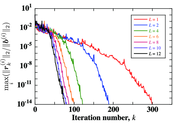
Figure 1: $L$ dependence of the convergence behaviors for the $j=12$ case. All the measurements are performed on the same configuration.

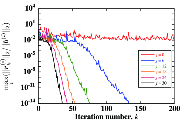
Figure 2: $j$ dependence of the convergence behaviors for the $L=12$ case. All the measurements are performed on the same configuration.

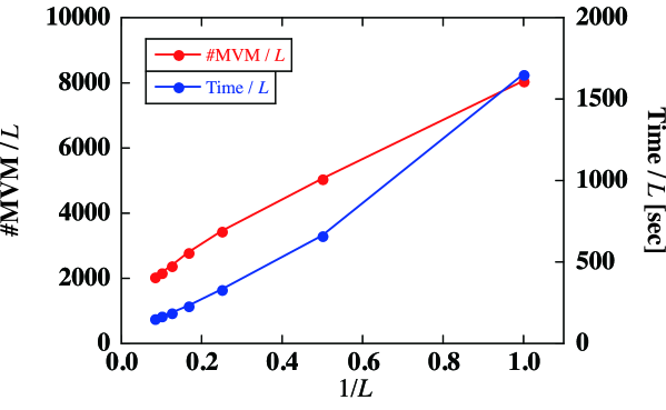
Figure 3: $L$ dependence of #MVM/$L$ (red) and the execution time divided by $L$ (blue) for the preconditioned block BiCGGR method with $j=12$. All the results are averaged over 10 configuration samples.

Table 2: Execution time divided by $L$ as a function of $L$ and the inner iteration number $j$ to solve the Wilson-Dirac equation with the preconditioned block BiCGGR method. Results are averaged over 10 configuration samples. Fail means how many configuration samples out of ten show the convergence failure.

$\kappa=0.1359$
$L$	$j=0$	$j=6$	$j=12$	$j=18$	$j=24$	$j=30$
$1$	$1511.0$	$1593.3$	$1649.6$	$1727.5$	$1773.9$	$1812.2$
$2$	$750.2$	$653.5$	$659.8$	$686.5$	$702.7$	$713.6$
$4$	Fail: $7$/$10$	Fail: $1$/$10$	$330.3$	$329.1$	$338.3$	$346.4$
$6$	Fail: $10$/$10$	$230.3$	$229.2$	$230.0$	$236.2$	$237.8$
$8$	Fail: $10$/$10$	Fail: $1$/$10$	$187.1$	$192.5$	$194.1$	$197.8$
$10$	Fail: $10$/$10$	Fail: $1$/$10$	$167.2$	$167.7$	$172.4$	$174.0$
$12$	Fail: $10$/$10$	$168.7$	$150.8$	$154.1$	$159.6$	Fail: $1$/$10$

4 Conclusions and discussions

In this paper we present an evidence that the convergence behavior of the block BiCGGR can be improved by the preconditioning technique. Our numerical tests show that the rank loss problem is remedied by the use of the inner solver with the Jacobi method as a preconditioner. As an optimized choice of $L$ and the inner iteration $j$ we can achieve 90% cost reduction in terms of the execution time.

There remains a couple of future works. Firstly, it is worthwhile to search a better preconditioner which assures the convergence for wider range of $L$ with less computational cost. Secondly, it is important to investigate why the preconditioner allows us to avoid the rank loss problem. Thirdly, we plan to apply the preconditioned block BiCGGR method to one of the state-of-the-art gauge configurations generated by the PACS-CS Collaboration[4]. Fourthly, it is interesting to make a direct comparison of the algorithmic efficiency between the preconditioned block BiCGGR method and other multiple right-hand-side methods[5, 6, 7, 8].

References

- [1] H. Tadano, T. Sakurai, Y. Kuramashi, Block BiCGGR: A New Block Krylov Subspace Method for Computing High Accuracy Solutions, JSIAM Letters (to be published).
- [2] T. Sakurai, H. Tadano, Y. Kuramashi, Application of Block Krylov Subspace Algorithms to the Wilson-Dirac Equation with Multiple Right-Hand Sides in Lattice QCD, arXiv:0903.4936 [hep-lat].
- [3] CP-PACS Collaboration, A. Ali Khan et al., Dynamical Quark Effects on Light Quark Masses, Phys. Rev. Lett. 85 (2000) 4674; Light Hadron Spectroscopy with Two Flavors of Dynamical Quarks on the Lattice, Phys. Rev. D65 (2002) 054505.
- [4] PACS-CS Collaboration, S. Aoki et al., 2+1 Flavor Lattice QCD toward the Physical Point, Phys. Rev. D 79, 034503 (2009).
- [5] M. Lüscher, Local Coherence and Deflation of the Low Quark Modes in Lattice QCD, JHEP 0707 (2007) 081.
- [6] A. Stathopoulos, K. Orginos, Computing and Deflating Eigenvalues While Solving Multiple Right Hand Side Linear Systems in Quantum Chromodynamics, arXiv:0707.0131 [hep-lat].
- [7] R. B. Morgan, W. Wilcox, Deflated Iterative Methods for Linear Equations with Multiple Right-Hand Sides, arXiv:0707.0505 [math-ph]; D. Darnell, R. B. Morgan, W. Wilcox, Deflated GMRES for Systems with Multiple Shifts and Multiple Right-Hand Sides, Linear Algebra Appl. 429 (2008) 2415; A. M. Abdel-Rehim, R. B. Morgan, D. A. Nicely, W. Wilcox, Deflated and Restarted Symmetric Lanczos Methods for Eigenvalues and Linear Equations with Multiple Right-hand Sides, arXiv:0806.3477 [math-ph]; A. M. Abdel-Rehim, R. B. Morgan, W. Wilcox, Improved Seed Methods for Symmetric Positive Definite Linear Equations with Multiple Right-hand Sides, arXiv:0810.0330 [math-ph].
- [8] J. Brannick, R. C. Brower, M. A. Clark, J. C. Osborn, C. Rebbi, Adaptive Multigrid Algorithm for Lattice QCD, Phys. Rev. Lett. 100 (2008) 041601.