Scaling limits of random planar maps with large faces

Abstract

We discuss asymptotics for large random planar maps under the assumption that the distribution of the degree of a typical face is in the domain of attraction of a stable distribution with index $\alpha\in(1,2)$. When the number $n$ of vertices of the map tends to infinity, the asymptotic behavior of distances from a distinguished vertex is described by a random process called the continuous distance process, which can be constructed from a centered stable process with no negative jumps and index $\alpha$. In particular, the profile of distances in the map, rescaled by the factor $n^{-1/2\alpha}$, converges to a random measure defined in terms of the distance process. With the same rescaling of distances, the vertex set viewed as a metric space converges in distribution as $n\to\infty$, at least along suitable subsequences, toward a limiting random compact metric space whose Hausdorff dimension is equal to $2\alpha$.

and

1 Introduction

The goal of the present work is to discuss the continuous limits of large random planar maps when the distribution of the degree of a typical face has a heavy tail. Recall that a planar map is a proper embedding of a finite connected graph in the two-dimensional sphere. For technical reasons, it is convenient to deal with rooted planar maps, meaning that there is a distinguished oriented edge called the root edge. One is interested in the “shape” of the graph and not in the particular embedding that is considered. More rigorously, two rooted planar maps are identified if they correspond via an orientation-preserving homeomorphism of the sphere. The faces of the map are the connected components of the complement of edges and the degree of a face counts the number of edges that are incident to it. Large random planar graphs are of particular interest in theoretical physics, where they serve as models of random geometry ADJ .

A simple way to generate a large random planar map is to choose it uniformly at random from the set of all rooted $p$-angulations with $n$ faces (a planar map is a $p$-angulation if all faces have degree $p$). It is conjectured that the scaling limit of uniformly distributed $p$-angulations with $n$ faces, when $n$ tends to infinity (or, equivalently, when the number of vertices tends to infinity), does not depend on the choice of $p$ and is given by the so-called Brownian map. Since the pioneering work of Chassaing and Schaeffer CSise , there have been several results supporting this conjecture. Marckert and Mokkadem MaMo introduced the Brownian map and proved a weak form of the convergence of rescaled uniform quadrangulations toward the Brownian map. A stronger version, involving convergence of the associated metric spaces in the sense of the Gromov–Hausdorff distance, was derived in Le Gall legall06 in the case of uniformly distributed $2p$-angulations. Because the distribution of the Brownian map has not been fully characterized, the convergence results of legall06 require the extraction of suitable subsequences. Proving the uniqueness of the distribution of the Brownian map is one of the key open problems in this area.

A more general way of choosing a large planar map at random is to use Boltzmann distributions. In this work, we restrict our attention to bipartite maps, where all face degrees are even. Given a sequence $q=(q_{1},q_{2},q_{3},\ldots)$ of nonnegative real numbers and a bipartite planar map $\mathbf{m}$, the associated Boltzmann weight is

$$W_{q}(\mathbf{m})=\prod_{f\in F(\mathbf{m})}q_{\operatorname{deg}(f)/2},$$ (1)

where $F(\mathbf{m})$ denotes the set of all faces of $\mathbf{m}$ and $\operatorname{deg}(f)$ is the degree of the face $f$. One can then generate a large planar map by choosing it at random from the set of all planar maps with $n$ vertices (or with $n$ faces) with probability weights that are proportional to $W_{q}(\mathbf{m})$. Such distributions arise naturally (possibly in slightly different forms) in problems involving statistical physics models on random maps. This is discussed in Section 8 below.

Assuming certain integrability conditions on the sequence of weights, Marckert and Miermont jfmgm05 obtain a variety of limit theorems for large random bipartite planar maps chosen according to these Boltzmann distributions. These results are extended in Miermont Mi1 and Miermont and Weill MW to the nonbipartite case, including large triangulations. In all of these papers, limiting distributions are described in terms of the Brownian map. Therefore, these results strongly suggest that the Brownian map should be the universal limit of large random planar maps, under the condition that the distribution of the degrees of faces satisfies some integrability property. Note that, even though the distribution of the Brownian map has not been characterized, many of its properties can be investigated in detail and have interesting consequences for typical large planar maps; see, in particular, the recent papers legall08 and Mi2 (and Bettinelli betti , for similar results, for random maps on surfaces of higher genus).

In the present work, we consider Boltzmann distributions such that, even for large $n$, a random planar map with $n$ vertices will have “macroscopic” faces, which, in some sense, will remain present in the scaling limit. This leads to a (conjectured) scaling limit which is different from the Brownian map. In fact, our limit theorems involve new random processes that are closely related to the stable trees of duqleg02 , in contrast to the construction of the Brownian map MaMo , legall06 , which is based on Aldous’ continuum random tree (CRT).

Let us informally describe our main results, referring to the following sections for more precise statements. For technical reasons, we consider planar maps that are both rooted and pointed (in addition to the root edge, there is a distinguished vertex, denoted by $v_{*}$). Roughly speaking, we choose the Boltzmann weights $q_{k}$ in (1) in such a way that the distribution of the degree of a (typical) face is in the domain of attraction of a stable distribution with index $\alpha\in(1,2)$. This can be made more precise by using the Bouttier–Di Francesco–Guitter bijection BdFGmobiles between bipartite planar maps and certain labeled trees called mobiles. A mobile is a (rooted) plane tree, where vertices at even distance (resp., odd distance) from the root are called white (resp., black) and white vertices are assigned integer labels that satisfy certain simple rules; see Section 3.1. In the Bouttier–Di Francesco–Guitter bijection, a (rooted and pointed) planar map $\mathbf{m}$ corresponds to a mobile $\theta(\mathbf{m})$ in such a way that each face of $\mathbf{m}$ is associated with a black vertex of $\theta(\mathbf{m})$ and each vertex of $\mathbf{m}$ (with the exception of the distinguished vertex $v_{*}$) is associated with a white vertex of $\theta(\mathbf{m})$. Moreover, the degree of a face of $\mathbf{m}$ is exactly twice the degree of the associated black vertex in the mobile $\theta(\mathbf{m})$ (see Section 3.1 for more details).

Under appropriate conditions on the sequence of weights $q$, formula (1) defines a finite measure $W_{q}$ on the set of all rooted and pointed planar maps. Moreover, if $\mathbf{P}_{q}$ is the probability measure obtained by normalizing $W_{q}$, then the mobile $\theta(\mathbf{m})$ associated with a planar map $\mathbf{m}$ distributed according to $\mathbf{P}_{q}$ is a critical two-type Galton–Watson tree, with different offspring distributions $\mu_{0}$ and $\mu_{1}$ for white and black vertices, respectively, and labels chosen uniformly over all possible assignments (see jfmgm05 and Proposition 4 below). The distribution $\mu_{0}$ is always geometric, whereas $\mu_{1}$ has a simple expression in terms of the weights $q_{k}$.

We now come to our basic assumption. In the present work, we choose the weights $q_{k}$ in such a way that $\mu_{1}(k)$ behaves like $k^{-\alpha-1}$, when $k\to\infty$, for some $\alpha\in(1,2)$. Recalling that the degree of a face of $\mathbf{m}$ is equal to twice the degree of the associated black vertex in the mobile $\theta(\mathbf{m})$, we see that, in a certain sense, the face degrees of a planar map distributed according to $\mathbf{P}_{q}$ are independent, with a common distribution that belongs to the domain of attraction of a stable law with index $\alpha$.

We equip the vertex set $V(\mathbf{m})$ of a planar map $\mathbf{m}$ with the graph distance $d_{\mathrm{gr}}$ and would like to investigate the properties of this metric space when $\mathbf{m}$ is distributed according to $\mathbf{P}_{q}$ and conditioned to be large. For every integer $n\geq 1$, denote by $M_{n}$ a random planar map distributed according to $\mathbf{P}_{q}(\cdot|\#V(\mathbf{m})=n)$. Our goal is to get information about typical distances in the metric space $(V(M_{n}),d_{\mathrm{gr}})$ when $n$ is large and, if at all possible, to prove that these (suitably rescaled) metric spaces converge in distribution as $n\to\infty$ in the sense of the Gromov–Hausdorff distance. As a motivation for studying the particular conditioning $\{\#V(\mathbf{m})=n\}$, we note that our results will have immediate application to Boltzmann distributions on nonpointed rooted planar maps: simply observe that a given rooted planar map with $n$ vertices corresponds to exactly $n$ different rooted and pointed planar maps.

To achieve the preceding goal, we use another nice feature of the Bouttier–Di Francesco–Guitter bijection: up to an additive constant depending on $\mathbf{m}$, the distance between $v_{*}$ and an arbitrary vertex $v\in V(\mathbf{m})\setminus\{v_{*}\}$ coincides with the label of the white vertex of $\theta(\mathbf{m})$ associated with $v$. Thus, in order to understand the asymptotic behavior of distances from $v_{*}$ in the map $M_{n}$, it suffices to get information about labels in the mobile $\theta(M_{n})$ when $n$ is large. To this end, we first consider the tree $\mathcal{T}(M_{n})$ obtained by ignoring the labels in $\theta(M_{n})$. Under our basic assumption, the results of duqleg02 can be applied to prove that the tree $\mathcal{T}(M_{n})$ converges in distribution, modulo a rescaling of distances by the factor $n^{-(1-1/\alpha)}$, toward the so-called stable tree with index $\alpha$. The stable tree can be defined by a suitable coding from the sample path of a centered stable Lévy process with no negative jumps and index $\alpha$, under an appropriate excursion measure. The preceding convergence to the stable tree is, however, not sufficient for our purposes since we are primarily interested in labels. Note that, under the assumptions made in jfmgm05 on the weight sequence $q$ (and, in particular, in the case of uniformly distributed $2p$-angulations), the rescaled trees $\mathcal{T}(M_{n})$ converge toward the CRT and the scaling limit of labels is described in jfmgm05 as Brownian motion indexed by the CRT or, equivalently, as the Brownian snake driven by a normalized Brownian excursion. In our “heavy tail” setting, however, the scaling limit of the labels is not Brownian motion indexed by the stable tree, but is given by a new random process of independent interest, which we call the continuous distance process.

Let us give an informal presentation of the distance process—a rigorous definition can be found in Section 4 below. We view the stable tree as the genealogical tree for a continuous population and the distance of a vertex from the root is interpreted as its generation in the tree. Fix a vertex $a$ in the stable tree. Among the ancestors of $a$, countably many of them, denoted by $b_{1},b_{2},\ldots,$ correspond to a sudden creation of mass in the population: each $b_{k}$ has a macroscopic number $\delta_{k}>0$ of “children” and one can also consider the quantity $r_{k}\in[0,\delta_{k}]$, which is the rank among these children of the one that is an ancestor of $a$. The preceding description is informal in our continuous setting (there are no children), but can be made rigorous thanks to the ideas developed in duqleg02 and, in particular, to the coding of the stable tree by a Lévy process. We then associate with each vertex $b_{k}$ a Brownian bridge $(B_{k}(t))_{t\in[0,\delta_{k}]}$ (starting and ending at $0$) with duration $\delta_{k}$, independently when $k$ varies, and we set

$$D(a)=\sum_{k=1}^{\infty}B_{k}(r_{k}).$$

The resulting process $D(a)$ when $a$ varies in the stable tree is the continuous distance process. As a matter of fact, since vertices of the stable tree are parametrized by the interval $[0,1]$ (using the coding by a Lévy process), it is more convenient to define the continuous distance process as a process $(D_{t})_{t\in[0,1]}$ indexed by the interval $[0,1]$ (or even by $\mathbb{R}_{+}$ when we consider a forest of trees).

Much of the technical work contained in this article is devoted to proving that the rescaled labels in the mobile $\theta(M_{n})$ converge in distribution to the continuous distance process. The proper rescaling of labels involves the multiplicative factor $n^{-1/2\alpha}$ instead of $n^{-1/4}$, as in earlier work. This indicates that the typical diameter of our random planar maps $M_{n}$ is of order $n^{1/2\alpha}$, rather than $n^{1/4}$ in the case of maps with faces of bounded degree. Because conditioning on the total number of vertices makes the proof more difficult, we first establish a version of the convergence of labels for a forest of independent mobiles having the distribution of $\theta(\mathbf{m})$ under $\mathbf{P}_{q}$. The proof of this result (Theorem 1) is given in Section 5. We then derive the desired convergence for the conditioned objects in Section 6.

Finally, we obtain asymptotic results for the planar maps $M_{n}$ in Section 7. Theorem 4 gives precise information about the profile of distances from the distinguished vertex $v_{*}$ in $M_{n}$. Precisely, let $\rho_{M_{n}}^{(n)}$ be the measure on $\mathbb{R}_{+}$ defined by

$$\int\rho_{M_{n}}^{(n)}({d}x)\varphi(x)=\frac{1}{n}\sum_{v\in V(M_{n})}\varphi(n^{-1/2\alpha}d_{\mathrm{gr}}(v_{*},v)).$$

Then, the sequence of random measures $\rho_{M_{n}}^{(n)}$ converges in distribution toward the measure $\rho^{(\infty)}$ defined by

$$\int\rho^{(\infty)}({d}x)\varphi(x)=\int_{0}^{1}{d}t\,\varphi\bigl{(}c(D_{t}-\underline{D})\bigr{)},$$

where $c>0$ is a constant depending on the sequence of weights and $\underline{D}=\min_{t\in[0,1]}D_{t}$.

We also investigate the convergence of the suitably rescaled metric spaces $V(M_{n})$ in the Gromov–Hausdorff sense. Theorem 5 shows that, at least along a subsequence, the random metric spaces $(V(M_{n}),n^{-1/2\alpha}d_{\mathrm{gr}})$ converge in distribution toward a limiting random compact metric space. Furthermore, the Hausdorff dimension of this limiting space is a.s. equal to $2\alpha$, which should be compared with the value $4$ for the dimension of the Brownian map legall06 . The fact that the Hausdorff dimension is bounded above by $2\alpha$ follows from Hölder continuity properties of the distance process that are established in Section 4. The proof of the corresponding lower bound is more involved and depends on some properties of the stable tree and its coding by Lévy processes, which are investigated in duqleg02 . Similarly as in the case of the convergence to the Brownian map, the extraction of a subsequence in Theorem 5 is needed because the limiting distribution is not characterized.

The paper is organized as follows. Section 2 introduces Boltzmann distributions on planar maps and formulates our basic assumption on the sequence of weights. Section 3 recalls the Bouttier–Di Francesco–Guitter bijection and the key result giving the distribution of the random mobile associated with a planar map under the Boltzmann distribution (Proposition 4). Section 3 also introduces several discrete functions coding mobiles, in terms of which most of the subsequent limit theorems are stated. Section 4 is devoted to the definition of the continuous distance process and to its Hölder continuity properties. In Section 5, we address the problem of the convergence of the discrete label process of a forest of random mobiles toward the continuous distance process of Section 4. We then deduce a similar convergence for labels in a single random mobile conditioned to be large in Section 6. Section 7 deals with the existence of scaling limits of large random planar maps and the calculation of the Hausdorff dimension of limiting spaces. Finally, Section 8 discusses some motivation coming from theoretical physics.

Notation

The symbols $K,K^{\prime},K_{1},K^{\prime}_{1},K_{2},\ldots$ will stand for positive constants that may depend on the choice of the weight sequence $q=(q_{1},q_{2},\ldots)$, but, unless otherwise indicated, do not depend on other quantities. The value of these constants may vary from one proof to another. The notation $C(\mathbb{R})$ stands for the space of all continuous functions from $\mathbb{R}_{+}$ into $\mathbb{R}$ and the notation $\mathbb{D}(\mathbb{R}^{d})$ stands for the Skorokhod space of all càdlàg functions from $\mathbb{R}_{+}$ into $\mathbb{R}^{d}$. If $X=(X_{t})_{t\geq 0}$ is a process with càdlàg paths, $X_{s-}$ denotes the left limit of $X$ at $s$ for every $s>0$. We denote the set of all finite measures on $\mathbb{R}_{+}$ by $M_{f}(\mathbb{R}_{+})$ and this set is equipped with the usual weak topology. If $(a_{k})$ and $(b_{k})$ are two sequences of positive numbers, the notation $a_{k}\sim b_{k}$ (as $k\to\infty$) means that the ratio $a_{k}/b_{k}$ tends to $1$ as $k\to\infty$. Unless otherwise indicated, all random variables and processes are defined on a probability space $(\Omega,\mathcal{F},\mathbb{P})$.

2 Critical Boltzmann laws on bipartite planar maps

2.1 Boltzmann distributions

A rooted and pointed bipartite map is a pair $(\mathbf{m},v_{*})$, where $\mathbf{m}$ is a rooted bipartite planar map and $v_{*}$ is a distinguished vertex of $\mathbf{m}$. As in Section 1, the graph distance on the vertex set $V(\mathbf{m})$ is denoted by $d_{\mathrm{gr}}$ and we let $e_{-},e_{+}$ be, respectively, the origin and the target of the root edge of $\mathbf{m}$. By the bipartite nature of $\mathbf{m}$, the quantities $d_{\mathrm{gr}}(e_{+},v_{*}),d_{\mathrm{gr}}(e_{-},v_{*})$ differ. Moreover, this difference is at most $1$ in absolute value since $e_{+}$ and $e_{-}$ are linked by an edge. We say that $(\mathbf{m},v_{*})$ is positive if

$$d_{\mathrm{gr}}(e_{+},v_{*})=d_{\mathrm{gr}}(e_{-},v_{*})+1.$$

It is called negative otherwise, that is, if $d_{\mathrm{gr}}(e_{+},v_{*})=d_{\mathrm{gr}}(e_{-},v_{*})-1$.

We let $\mathcal{M}_{+}^{*}$ denote the set of all rooted and pointed bipartite planar maps that are positive. In the sequel, the mention of $v_{*}$ will usually be implicit, so we will simply denote the generic element of $\mathcal{M}_{+}^{*}$ by $\mathbf{m}$. For our purposes, it is useful to add an element $\dagger$ to $\mathcal{M}_{+}^{*}$, which can be seen roughly as the vertex map with no edge and a single vertex $v_{*}$ “bounding” a single face of degree $0$.

Let $q=(q_{1},q_{2},\ldots)$ be a sequence of nonnegative real numbers. For every $\mathbf{m}\in\mathcal{M}_{+}^{*}\setminus\{\dagger\}$, set

$$W_{q}(\mathbf{m})=\prod_{f\in F(\mathbf{m})}q_{\operatorname{deg}(f)/2},$$

where $F(\mathbf{m})$ denotes the set of all faces of $\mathbf{m}$. By convention, we set $W_{q}(\dagger)=1$. This defines a $\sigma$-finite measure on $\mathcal{M}_{+}^{*}$, whose total mass is

$$Z_{q}=W_{q}(\mathcal{M}_{+}^{*})\in[1,\infty].$$

We say that $q$ is admissible if $Z_{q}<\infty$, in which case we can define $\mathbf{P}_{q}=Z_{q}^{-1}W_{q}$ as the probability measure obtained by normalizing $W_{q}$. The measure $\mathbf{P}_{q}$ is called the Boltzmann distribution on $\mathcal{M}_{+}^{*}$ with weight sequence $q$.

Following jfmgm05 , we have the following simple criterion for the admissibility of $q$. Introduce the function

$$f_{q}(x)=\sum_{k=1}^{\infty}N(k)q_{k}x^{k-1},\qquad x\geq 0,$$ (2)

where

$$N(k)=\pmatrix{{2k-1}\cr{k-1}}.$$

Let $R_{q}\geq 0$ be the radius of convergence of this power series. Note that by monotone convergence, the quantity $f_{q}(R_{q})=f_{q}(R_{q}-)\in[0,\infty]$ exists, as well as $f^{\prime}_{q}(R_{q})=f^{\prime}_{q}(R_{q}-)$.

Proposition 1 (jfmgm05 ).

The sequence $q$ is admissible if and only if the equation

$$f_{q}(x)=1-\frac{1}{x},\qquad x\geq 1,$$ (3)

has a solution. If this holds, then the smallest such solution equals $Z_{q}$.

On the interval $[0,R_{q})$, the function $f_{q}$ is convex, so the equation (3) has at most two solutions. Let us now pause for a short informal discussion, inspired by jfmgm05 . For a “typical” admissible sequence $q$, the graphs of $f_{q}$ and of the function $x\mapsto 1-1/x$ will cross at $x=Z_{q}$ without being tangent. In this case, the law of the number of vertices of a $\mathbf{P}_{q}$-distributed random map will have an exponential tail. An admissible sequence $q$ is called critical if the graphs are tangent at $Z_{q}$, that is, if

$$Z_{q}^{2}f_{q}^{\prime}(Z_{q})=1.$$ (4)

For critical sequences, the law of the number of vertices of a $\mathbf{P}_{q}$-distributed random map may have a tail heavier than exponential. In the case where $R_{q}>Z_{q}$, jfmgm05  shows that this tail follows a power law with exponent $-1/2$. However, the law of the degree of a typical face in such a random map will have an exponential tail.

In the present paper, we will be interested in the “extreme” cases where $q$ is a critical sequence such that $Z_{q}=R_{q}$. We will show that in a number of these cases, the degree of a typical face in a $\mathbf{P}_{q}$-distributed random map also has a heavy tail distribution.

2.2 Choosing the Boltzmann weights

We start from a sequence $q^{\circ}:=(q_{k}^{\circ})_{k\in\mathbb{N}}$ of nonnegative real numbers such that

$$q_{k}^{\circ}\mathop{\sim}_{k\to\infty}k^{-a}$$ (5)

for some real number $a>3/2$. In agreement with (2), we set

$$f_{\circ}(x)=f_{q^{\circ}}(x)=\sum_{k=1}^{\infty}N(k)q^{\circ}_{k}x^{k-1}$$

for every $x\geq 0$. By Stirling’s formula, we have

$$N(k)\mathop{\sim}_{k\to\infty}\frac{2^{2k-1}}{\sqrt{\pi k}}$$

so that the radius of convergence of the series defining $f_{\circ}$ is $1/4$. Furthermore, the condition $a>3/2$ guarantees that $f_{\circ}(1/4)$ and $f^{\prime}_{\circ}(1/4)$ are (well defined and) finite.

Proposition 2.

Set

$$c=\frac{4}{4f_{\circ}(1/4)+f^{\prime}_{\circ}(1/4)},\qquad\beta=\frac{f^{\prime}_{\circ}(1/4)}{4f_{\circ}(1/4)+f^{\prime}_{\circ}(1/4)}$$

and define a sequence $q=(q_{k})_{k\in\mathbb{N}}$ by setting

$$q_{k}=c(\beta/4)^{k-1}q^{\circ}_{k}.$$ (6)

Then, the sequence $q$ is both admissible and critical, and $Z_{q}=R_{q}=\beta^{-1}$.

As the proof will show, the choice given for the constants $c$ and $\beta$ is the only one for which the conclusion of the proposition holds. Proof of Proposition 2 Consider a sequence $q=(q_{k})_{k\in\mathbb{N}}$ defined as in the proposition, with an arbitrary choice of the positive constants $c$ and $\beta$. If $f_{q}$ is defined as in (2), it is immediate that

$$f_{q}(x)=cf_{\circ}(\beta x/4).$$

Hence, $R_{q}=\beta^{-1}$. Assume, for the moment, that the sequence $q$ is admissible and $Z_{q}=R_{q}$. By Proposition 1, we have $f_{q}(\beta^{-1})=1-\beta$ or, equivalently,

$$cf_{\circ}(1/4)=1-\beta.$$ (7)

Furthermore, the criticality of $q$ will hold if and only if $f^{\prime}_{q}(\beta^{-1})=\beta^{2}$ or, equivalently,

$$cf^{\prime}_{\circ}(1/4)=4\beta.$$ (8)

Conversely, if (7) and (8) both hold, then the sequence $q$ is admissible by Proposition 1, the curves $x\to f_{q}(x)$ and $x\to 1-1/x$ are tangent at $x=\beta^{-1}$ and a simple convexity argument shows that $\beta^{-1}$ is the unique solution of (3) so that $Z_{q}=\beta^{-1}=R_{q}$, again by Proposition 1.

We conclude that the conditions (7) and (8) are necessary and sufficient for the conclusion of the proposition to hold. The desired result thus follows.

We now introduce our basic assumption, placing a further restriction on the value of the parameter $a$.

Assumption (A).

The sequence $q$ is of the form given in Proposition 2, with a sequence $q^{\circ}$ satisfying (5) for some $a\in(3/2,5/2)$. We set $\alpha:=a-1/2\in(1,2)$.

This assumption will be in force throughout the remainder of this work, with the exception of the beginning of Section 3.2 (including Proposition 4), where we consider a general admissible sequence $q$.

Many of the subsequent asymptotic results will be written in terms of the constant $\beta$, which lies in the interval $(0,1)$, and the constant $c_{0}>0$ defined by

$$c_{0}=\biggl{(}\frac{2c\Gamma(2-\alpha)}{\alpha(\alpha-1)\beta\sqrt{\pi}}\biggr{)}^{1/\alpha}.$$ (9)

The reason for introducing this other constant will become clearer in Section 3.2.

3 Coding maps with mobiles

3.1 The Bouttier–Di Francesco–Guitter bijection

Following BdFGmobiles , we now recall how bipartite planar maps can be coded by certain labeled trees called mobiles.

By definition, a plane tree $\mathcal{T}$ is a finite subset of the set

$$\mathcal{U}=\bigcup_{n\geq 0}^{\infty}\mathbb{N}^{n}$$ (10)

of all finite sequences of positive integers (including the empty sequence $\varnothing$) which satisfies three obvious conditions. First, $\varnothing\in\mathcal{T}$. Then, for every $v=(u_{1},\ldots,u_{k})\in\mathcal{T}$ with $k\geq 1$, the sequence $(u_{1},\ldots,u_{k-1})$ (the “parent” of $v$) also belongs to $\mathcal{T}$. Finally, for every $v=(u_{1},\ldots,u_{k})\in\mathcal{T}$, there exists an integer $k_{v}(\mathcal{T})\geq 0$ (the “number of children” of $v$) such that $vj:=(u_{1},\ldots,u_{k},j)$ belongs to $\mathcal{T}$ if and only if $1\leq j\leq k_{v}(\mathcal{T})$. The elements of $\mathcal{T}$ are called vertices. The generation of a vertex $v=(u_{1},\ldots,u_{k})$ is denoted by $|v|=k$. The notions of an ancestor and a descendant in the tree $\mathcal{T}$ are defined in an obvious way.

For our purposes, vertices $v$ such that $|v|$ is even will be called white vertices and vertices $v$ such that $|v|$ is odd will be called black vertices. We denote by $\mathcal{T}^{\circ}$ (resp., $\mathcal{T}^{\bullet}$) the set of all white (resp., black) vertices of $\mathcal{T}$.

A (rooted) mobile is a pair $\theta=(\mathcal{T},(\ell(v))_{v\in\mathcal{T}^{\circ}})$ that consists of a plane tree and a collection of integer labels assigned to the white vertices of $\mathcal{T}$ such that the following properties hold:

1. [(a)]

2. $\ell(\varnothing)=0$.

3. Let $v\in\mathcal{T}^{\bullet}$, $v_{(0)}$ be the parent of $v$, $p=k_{v}(\mathcal{T})+1$ and $v_{(j)}=vj$, $1\leq j\leq p-1$ be the children of $v$. Then, for every $j\in\{1,\ldots,p\}$, $\ell(v_{(j)})\geq\ell(v_{(j-1)})-1$, where, by convention, $v_{(p)}=v_{(0)}$.

Condition (b) means that if one lists the white vertices adjacent to a given black vertex in clockwise order, then the labels of these vertices can decrease by at most 1 at each step. See Figure 1 for an example of a mobile.

Figure 1: A rooted mobile.

We denote by $\Theta$ the (countable) set of all mobiles. We will now describe the Bouttier–Di Francesco–Guitter (BDG) bijection between $\Theta$ and $\mathcal{M}_{+}^{*}$. This bijection can be found in Section 2 of BdFGmobiles , with the minor difference that BdFGmobiles deals with maps that are pointed, but not rooted.

Let $\theta=(\mathcal{T},(\ell(v))_{v\in\mathcal{T}^{\circ}})$ be a mobile with $n+1$ vertices. The contour sequence of $\theta$ is the sequence $v_{0},\ldots,v_{2n}$ of vertices of $\mathcal{T}$ which is obtained by induction as follows. First, $v_{0}=\varnothing$ and then, for every $i\in\{0,\ldots,2n-1\}$, $v_{i+1}$ is either the first child of $v_{i}$ that has not yet appeared in the sequence $v_{0},\ldots,v_{i}$ or the parent of $v_{i}$ if all children of $v_{i}$ already appear in the sequence $v_{0},\ldots,v_{i}$. It is easy to verify that $v_{2n}=\varnothing$ and that all vertices of $\mathcal{T}$ appear in the sequence $v_{0},v_{1},\ldots,v_{2n}$. In fact, a given vertex $v$ appears exactly $k_{v}(\mathcal{T})+1$ times in the contour sequence and each appearance of $v$ corresponds to one “corner” associated with this vertex.

The vertex $v_{i}$ is white when $i$ is even and black when $i$ is odd. The contour sequence of $\mathcal{T}^{\circ}$, also called the white contour sequence of $\theta$, is, by definition, the sequence $v^{\circ}_{0},\ldots,v^{\circ}_{n}$ defined by $v^{\circ}_{i}=v_{2i}$ for every $i\in\{0,1,\ldots,n\}$.

The image of $\theta$ under the BDG bijection is the element $(\mathbf{m},v_{*})$ of $\mathcal{M}_{+}^{*}$ that is defined as follows. First, if $n=0$, meaning that $\mathcal{T}=\{\varnothing\}$, we set $(\mathbf{m},v_{*})=\dagger$. Suppose that $n\geq 1$ so that $\mathcal{T}^{\bullet}$ has at least one element. We extend the white contour sequence of $\theta$ to a sequence $v^{\circ}_{i}$, $i\geq 0$, by periodicity, in such a way that $v^{\circ}_{i+n}=v^{\circ}_{i}$ for every $i\geq 0$. Then, suppose that the tree $\mathcal{T}$ is embedded in the plane and add an extra vertex $v_{*}$ not belonging to the embedding. We construct a rooted planar map $\mathbf{m}$ whose vertex set is equal to

$$V(\mathbf{m})=\mathcal{T}^{\circ}\cup\{v_{*}\}$$

and whose edges are obtained by the following device. For $i\in\{0,1,\ldots,n-1\}$, we let

$$\phi(i)=\inf\{j>i\dvtx\ell(v^{\circ}_{j})=\ell(v^{\circ}_{i})-1\}\in\{i+1,i+2,\ldots\}\cup\{\infty\}.$$

We also set $v^{\circ}_{\infty}=v_{*}$, by convention. Then, for every $i\in\{0,1,\ldots,n-1\}$, we draw an edge between $v^{\circ}_{i}$ and $v^{\circ}_{\phi(i)}$. More precisely, the index $i$ corresponds to one specific “corner” of $v^{\circ}_{i}$ and the associated edge starts from this corner. The construction can then be made in such a way that edges do not cross (and do not cross the edges of the tree) so that one indeed gets a planar map. This planar map $\mathbf{m}$ is rooted at the edge linking $v^{\circ}_{0}=\varnothing$ to $v^{\circ}_{\phi(0)}$, which is oriented from $v^{\circ}_{\phi(0)}$ to $\varnothing$. Furthermore, $\mathbf{m}$ is pointed at the vertex $v_{*}$, in agreement with our previous notation.

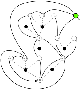
Figure 2: The Bouttier–Di Francesco–Guitter construction for the mobile of Figure 1.

See Figure 2 for an example and Section 2 of BdFGmobiles for a more detailed description.

Proposition 3 ((BDG bijection)).

The preceding construction yields a bijection from $\Theta$ onto $\mathcal{M}_{+}^{*}$. This bijection enjoys the following two properties:

1. each face $f$ of $\mathbf{m}$ contains exactly one vertex $v$ of $\mathcal{T}^{\bullet}$, with $\deg(f)=2(k_{v}(\mathcal{T})+1)$;

2. the graph distances in $\mathbf{m}$ to the distinguished vertex $v_{*}$ are linked to the labels of the mobile in the following way: for every $v\in\mathcal{T}^{\circ}=V(\mathbf{m})\setminus\{v_{*}\}$,

   $$d_{\mathrm{gr}}(v_{*},v)=\ell(v)-\min_{v^{\prime}\in\mathcal{T}^{\circ}}\ell(v^{\prime})+1.$$

In our study of scaling limits of random planar maps, it will be important to derive asymptotics for the random mobiles associated with these maps via the BDG bijection. These asymptotics are more conveniently stated in terms of random processes coding the mobiles. Let us introduce such coding functions.

Let $\theta=(\mathcal{T},(\ell(v))_{v\in\mathcal{T}^{\circ}})$ be a mobile with $n+1$ vertices (so that $n=\#\mathcal{T}-1$) and let $v^{\circ}_{0},\ldots,v^{\circ}_{n}$ be, as previously, the white contour sequence of $\theta$. We set

$$C^{\theta}_{i}=\tfrac{1}{2}|v^{\circ}_{i}|\qquad\mbox{for }0\leq i\leq n,\qquad C^{\theta}_{i}=0\qquad\mbox{for }i>n.$$ (11)

We call $(C^{\theta}_{i},0\leq i\leq n)$ the contour process of the mobile $\theta$. It is a simple exercise to check that the contour process $C^{\theta}$ determines the tree $\mathcal{T}$. Similarly, we set

$$\Lambda^{\theta}_{i}=\ell(v^{\circ}_{i})\qquad\mbox{for }0\leq i\leq n,\qquad\Lambda^{\theta}_{i}=0\qquad\mbox{for }i>n$$ (12)

and call $\Lambda^{\theta}$ the contour label process of $\theta$. The pair $(C^{\theta},\Lambda^{\theta})$ determines the mobile $\theta$.

For technical reasons, we introduce variants of the preceding contour functions. Let $n_{\circ}=\#\mathcal{T}^{\circ}-1$ and let $w^{\circ}_{0}=\varnothing,w^{\circ}_{1},\ldots,w^{\circ}_{n_{\circ}}$, be the list of vertices of $\mathcal{T}^{\circ}$ in lexicographical order. The height process of $\theta$ is defined by

$$H^{\theta}_{i}=\tfrac{1}{2}|w^{\circ}_{i}|\qquad\mbox{for }0\leq i\leq n_{\circ},\qquad H^{\theta}_{i}=0\qquad\mbox{for }i>n_{\circ}.$$

Similarly, we introduce the label process, which is defined by

$$L^{\theta}_{i}=\ell(w^{\circ}_{i})\qquad\mbox{for }0\leq i\leq n_{\circ},\qquad L^{\theta}_{i}=0\qquad\mbox{for }i>n_{\circ}.$$

We will also need the Lukasiewicz path of $\mathcal{T}^{\circ}$. This is the sequence $S^{\theta}=(S^{\theta}_{0},S^{\theta}_{1},\ldots)$, defined as follows. First, $S^{\theta}_{0}=0$. Then, for every $i\in\{0,1,\ldots,n_{\circ}\}$, $S^{\theta}_{i+1}-S^{\theta}_{i}+1$ is the number of (white) grandchildren of $w^{\circ}_{i}$ in $\mathcal{T}$. Finally, $S^{\theta}_{i}=S^{\theta}_{n_{\circ}+1}=-1$ for every $i>n_{\circ}$. It is easy to see that $S^{\theta}_{i}\geq 0$ for every $i\in\{0,1,\ldots,n_{\circ}\}$ so that

$$\#\mathcal{T}^{\circ}=n_{\circ}+1=\inf\{i\geq 0\dvtx S^{\theta}_{i}=-1\}.$$

Let us briefly comment on the reason for introducing these different processes. In our applications to random planar maps, asymptotics for the pair $(C^{\theta},\Lambda^{\theta})$, which is directly linked to the white contour sequence of $\theta$, turn out to be most useful. On the other hand, in order to derive these asymptotics, it will be more convenient to consider first the pair $(H^{\theta},L^{\theta})$.

In the following, the generic element of $\Theta$ will be denoted by $(\theta,(\ell(v))_{v\in\mathcal{T}^{\circ}}),$ as previously.

3.2 Boltzmann distributions and Galton–Watson trees

Let $q$ be an admissible sequence, in the sense of Section 2, and let $M$ be a random element of $\mathcal{M}_{+}^{*}$ with distribution $\mathbf{P}_{q}$. Our goal is to describe the distribution of the random mobile associated with $M$ via the BDG bijection. We closely follow Section 2.2 of jfmgm05 .

We first need the notion of an alternating two-type Galton–Watson tree. Recall that white vertices are those of even generation and black vertices are those of odd generation. Informally, an alternating two-type Galton–Watson tree is just a Galton–Watson tree where white and black vertices have a different offspring distribution. More precisely, if $\mu_{0}$ and $\mu_{1}$ are two probability distributions on the nonnegative integers, the associated (alternating) two-type Galton–Watson tree is the random plane tree whose distribution is specified by saying that the numbers of children of the different vertices are independent, the offspring distribution of each white vertex is $\mu_{0}$ and the offspring distribution of each black vertex is $\mu_{1}$; see jfmgm05 , Section 2.2, for a more rigorous presentation.

We also need to introduce the notion of a discrete bridge. Consider an integer $p\geq 1$ and the set

$$E_{p}:=\Biggl{\{}(x_{1},\ldots,x_{p})\in\{-1,0,1,2,\ldots\}^{p}\dvtx\sum_{i=1}^{p}x_{i}=0\Biggr{\}}.$$

Note that $E_{p}$ is a finite set and, indeed, $\#E_{p}=N(p)$, with $N(p)$ as in (2). Let $(X_{1},\ldots,X_{p})$ be uniformly distributed over $E_{p}$. The sequence $(Y_{0},Y_{1},\ldots,Y_{p})$ defined by $Y_{0}=0$ and

$$Y_{j}=\sum_{i=1}^{j}X_{i},\qquad 1\leq j\leq p,$$

is called a discrete bridge of length $p$.

Proposition 4 ((jfmgm05 , Proposition 7)).

Let $M$ be a random element of $\mathcal{M}_{+}^{*}$ with distribution $\mathbf{P}_{q}$ and let $\theta=(\mathcal{T},(\ell(v),v\in\mathcal{T}^{\circ}))$ be the random mobile associated with $M$ via the BDG bijection. Then:

1. the random tree $\mathcal{T}$ is an alternating two-type Galton–Watson tree with offspring distributions $\mu_{0}$ and $\mu_{1}$ given by

   $$\mu_{0}(k)=Z_{q}^{-1}f_{q}(Z_{q})^{k},\qquad k\geq 0,$$

   and

   $$\mu_{1}(k)=\frac{Z_{q}^{k}N(k+1)q_{k+1}}{f_{q}(Z_{q})},\qquad k\geq 0;$$

2. conditionally given $\mathcal{T}$, the labels $(\ell(v),v\in\mathcal{T}^{\circ})$ are distributed uniformly over all possible choices that satisfy the constraints (a) and (b) in the definition of a mobile; equivalently, for every $v\in\mathcal{T}^{\bullet}$, with the notation introduced in property (b) of the definition of a mobile, the sequence $(\ell(v_{(j)})-\ell(v_{(0)}),0\leq j\leq k_{v}(\mathcal{T})+1)$ is a discrete bridge of length $k_{v}(\mathcal{T})+1$ and these sequences are independent when $v$ varies over $\mathcal{T}^{\bullet}$.

A random mobile having the distribution described in the proposition will be called a $(\mu_{0},\mu_{1})$-mobile. The law $\mathbb{Q}$ of a $(\mu_{0},\mu_{1})$-mobile is a probability distribution on $\Theta$.

Note that the respective means of $\mu_{0}$ and $\mu_{1}$ are

$$m_{0}:=\sum_{k\geq 0}k\mu_{0}(k)=Z_{q}f_{q}(Z_{q}),\qquad m_{1}:=\sum_{k\geq 0}k\mu_{1}(k)=Z_{q}f_{q}^{\prime}(Z_{q})/f_{q}(Z_{q})$$

so that $m_{0}m_{1}=Z_{q}^{2}f^{\prime}_{q}(Z_{q})$ is less than or equal to $1$ and equality holds if and only if $q$ is critical.

We now return to a weight sequence $q$ satisfying our basic Assumption (A). Recall that the sequence $q$, which is both admissible and critical, is given in terms of the sequence $q^{\circ}$ by (6) and that we have $q^{\circ}_{k}\sim k^{-\alpha-1/2}$ as $k\to\infty$, with $\alpha\in(1,2)$.

Then, $\mu_{0}$ is the geometric distribution with parameter $f_{q}(Z_{q})=1-\beta$ and

$$\mu_{1}(k)=\frac{c}{1-\beta}4^{-k}N(k+1)q^{\circ}_{k+1},\qquad k=0,1,\ldots.$$

From the asymptotic behavior of $q^{\circ}_{k}$, we obtain

$$\mu_{1}(k)\mathop{\sim}_{k\to\infty}\frac{2c}{(1-\beta)\sqrt{\pi}}k^{-\alpha-1}.$$

In particular, if we set $\overline{\mu}_{1}(k)=\mu_{1}([k,\infty))$, this yields

$$\overline{\mu}_{1}(k)\mathop{\sim}_{k\to\infty}\frac{2c}{\alpha(1-\beta)\sqrt{\pi}}k^{-\alpha}.$$ (13)

Let $\mu$ be the probability distribution on the nonnegative integers which is the law of

$$\sum_{i=1}^{U}V_{i},$$

where $U$ is distributed according to $\mu_{0}$, $V_{1},V_{2},\ldots$ are distributed according to $\mu_{1}$ and the variables $U,V_{1},V_{2},\ldots$ are independent. Then, $\mu$ is critical, in the sense that

$$\sum_{k=0}^{\infty}k\mu(k)=m_{0}m_{1}=1.$$

Notice that $\mu$ is just the distribution of the number of individuals at the second generation of a $(\mu_{0},\mu_{1})$-mobile. It will be important to have information on the tail $\overline{\mu}(k):=\mu([k,\infty))$ of $\mu$. This follows easily from the estimate (13) and the definition of $\mu$. First, note that

$$\overline{\mu}(k)=\mathbb{P}\Biggl{[}\sum_{i=1}^{U}V_{i}\geq k\Biggr{]}\geq\mathbb{P}[\exists i\in\{1,\ldots,U\}\dvtx V_{i}\geq k]=1-\mathbb{E}\bigl{[}\bigl{(}1-\overline{\mu}_{1}(k)\bigr{)}^{U}\bigr{]}.$$

Then,

$$1-\mathbb{E}\bigl{[}\bigl{(}1-\overline{\mu}_{1}(k)\bigr{)}^{U}\bigr{]}=1-\frac{\beta}{1-(1-\overline{\mu}_{1}(k))(1-\beta)}\mathop{\sim}_{k\to\infty}\frac{1-\beta}{\beta}\overline{\mu}_{1}(k).$$

Using (13), we get

$$\overline{\mu}(k)\geq\frac{2c}{\alpha\beta\sqrt{\pi}}k^{-\alpha}+o(k^{-\alpha}).$$

A corresponding upper bound is easily obtained by writing, for every $\varepsilon\in(0,1/2)$,

$$\overline{\mu}(k) \leq \mathbb{P}[\exists i\in\{1,\ldots,U\}\dvtx V_{i}\geq(1-\varepsilon)k]$$

$${}+\mathbb{P}\Biggl{[}\Biggl{\{}\sum_{i=1}^{U}V_{i}\geq k\Biggr{\}}\cap\bigl{\{}\forall i\in\{1,\ldots,U\}\dvtx V_{i}\leq(1-\varepsilon)k\bigr{\}}\Biggr{]}$$

and checking that the second term in the right-hand side is $o(k^{-\alpha})$ as $k\to\infty$. To see this, first note that the probability of the event $\{U>K\log k\}$ is $o(k^{-\alpha})$ if the constant $K$ is chosen sufficiently large. If $U\leq K\log k$, then the event in the second term may hold only if there are two distinct values of $i\in\{1,2,\ldots,[K\log k]\}$ such that $V_{i}\geq\varepsilon k/(K\log k)$. The desired estimate then follows from (13).

We have thus obtained

$$\overline{\mu}(k)\mathop{\sim}_{k\to\infty}\frac{2c}{\alpha\beta\sqrt{\pi}}k^{-\alpha},$$

which we can rewrite in the form

$$\overline{\mu}(k)\mathop{\sim}_{k\to\infty}\frac{\alpha-1}{\Gamma(2-\alpha)}c_{0}^{\alpha}k^{-\alpha}$$ (14)

with the constant $c_{0}$ defined in (9). The reason for introducing the constant $c_{0}$ and writing the asymptotics (14) in this form becomes clear when discussing scaling limits. Recall that $1<\alpha<2$ by our assumption that $\frac{3}{2}<a<\frac{5}{2}$. By (13) or (14), $\mu$ is then in the domain of attraction of a stable law with index $\alpha$. Recalling that $\mu$ is critical, we have the following, more precise, result.

Let $\nu$ be the probability distribution on $\mathbb{Z}$ obtained by setting $\nu(k)=\mu(k+1)$ for every $k\geq-1$ [and $\nu(k)=0$ if $k<-1$]. Let $S=(S_{n})_{n\geq 0}$ be a random walk on the integers with jump distribution $\nu$. Then,

$$\bigl{(}n^{-1/\alpha}S_{[nt]}\bigr{)}_{t\geq 0}\mathop{\longrightarrow}_{n\to\infty}^{\mathrm{(d)}}(c_{0}X_{t})_{t\geq 0},$$ (15)

where the convergence holds in distribution in the Skorokhod sense and $X$ is a centered stable Lévy process with index $\alpha$ and no negative jumps, with Laplace transform given by

$$\mathbb{E}[\exp(-uX_{t})]=\exp(tu^{\alpha}),\qquad t,u\geq 0.$$ (16)

See, for instance, Chapter VII of Jacod and Shiryaev JS for a thorough discussion of the convergence of rescaled random walks toward Lévy processes.

3.3 Discrete bridges

Recall from Proposition 4 that the sequence of labels of white vertices adjacent to a given black vertex in a $(\mu_{0},\mu_{1})$-mobile is distributed as a discrete bridge. In this section, we collect some estimates for discrete bridges that will be used in the proofs of our main results.

We consider a random walk $(Y_{n})_{n\geq 0}$ on $\mathbb{Z}$ starting from $0$ and with jump distribution

$$\nu_{*}(k)=2^{-k-2},\qquad k=-1,0,1,\ldots.$$

Fix an integer $p\geq 1$ and let $(Y^{(p)}_{n})_{0\leq n\leq p}$ be a vector whose distribution is the conditional law of $(Y_{n})_{0\leq n\leq p}$ given that $Y_{p}=0$. Then, the process $(Y^{(p)}_{n})_{0\leq n\leq p}$ is a discrete bridge with length $p$. Indeed, a simple calculation shows that

$$\bigl{(}Y^{(p)}_{1},Y^{(p)}_{2}-Y^{(p)}_{1},\ldots,Y^{(p)}_{p}-Y^{(p)}_{p-1}\bigr{)}$$

is uniformly distributed over the set $E_{p}$.

Lemma 1.

For every real $r\geq 1$, there exists a constant $K_{(r)}$ such that for every integer $p\geq 1$ and $k,k^{\prime}\in\{0,1,\ldots,p\}$,

$$\mathbb{E}\bigl{[}\bigl{(}Y^{(p)}_{k}-Y^{(p)}_{k^{\prime}}\bigr{)}^{2r}\bigr{]}\leq K_{(r)}|k-k^{\prime}|^{r}.$$

We may, and will, assume that $p\geq 2$. Let us first suppose that $k\leq k^{\prime}\leq 2p/3$. By the definition of $Y^{(p)}$ and then the Markov property of $Y$, we have

$$\mathbb{E}\bigl{[}\bigl{(}Y^{(p)}_{k}-Y^{(p)}_{k^{\prime}}\bigr{)}^{2r}\bigr{]}=\frac{\mathbb{E}[|Y_{k}-Y_{k^{\prime}}|^{2r}\mathbh{1}_{\{Y_{p}=0\}}]}{\mathbb{P}(Y_{p}=0)}=\mathbb{E}\biggl{[}|Y_{k}-Y_{k^{\prime}}|^{2r}\frac{\pi_{p-k^{\prime}}(-Y_{k^{\prime}})}{\pi_{p}(0)}\biggr{]},$$

where $\pi_{n}(x)=\mathbb{P}(Y_{n}=x)$ for every integer $n\geq 0$ and $x\in\mathbb{Z}$. A standard local limit theorem (see, e.g., Section 7 of spitzer ) shows that if $g(x)=(4\pi)^{-1/2}e^{-x^{2}/4}$, then we have

$$\sqrt{n}\pi_{n}(x)=g\bigl{(}x/\sqrt{n}\bigr{)}+\varepsilon_{n}(x)\qquad\mbox{where }\sup_{x\in\mathbb{Z}}|\varepsilon_{n}(x)|\mathop{\to}_{n\to\infty}0.$$

Then,

$$\frac{\pi_{p-k^{\prime}}(-Y_{k^{\prime}})}{\pi_{p}(0)}\leq\sqrt{3}\frac{\sqrt{p-k^{\prime}}\pi_{p-k^{\prime}}(-Y_{k^{\prime}})}{\sqrt{p}\pi_{p}(0)}\leq K,$$

where

$$K=\sqrt{3}\frac{(4\pi)^{-1/2}+\sup_{n\geq 1}\sup_{x\in\mathbb{Z}}|\varepsilon_{n}(x)|}{\inf_{n\geq 1}\sqrt{n}\pi_{n}(0)}<\infty.$$

It follows that

$$\mathbb{E}\bigl{[}\bigl{(}Y^{(p)}_{k}-Y^{(p)}_{k^{\prime}}\bigr{)}^{2r}\bigr{]}\leq K\mathbb{E}[|Y_{k}-Y_{k^{\prime}}|^{2r}].$$

Then, the bound $\mathbb{E}[|Y_{k}-Y_{k^{\prime}}|^{2r}]\leq K^{\prime}_{(r)}|k-k^{\prime}|^{r},$ with a finite constant $K^{\prime}_{(r)}$ depending only on $r$, is a consequence of Rosenthal’s inequality for i.i.d. centered random variables petrov75 , Theorem 2.10. We have thus obtained the desired estimate under the restriction $k\leq k^{\prime}\leq 2p/3$.

If $p/3\leq k\leq k^{\prime}\leq p$, the same estimate is readily obtained by observing that $(-Y^{(p)}_{p-n},0\leq n\leq p)$ has the same distribution as $Y^{(p)}$. Finally, in the case $k\leq p/3\leq 2p/3\leq k^{\prime}$, we apply the preceding bounds successively to $\mathbb{E}[|Y_{k}-Y_{[p/2]}|^{2r}]$ and to $\mathbb{E}[|Y_{[p/2]}-Y_{k^{\prime}}|^{2r}]$.

An immediate consequence of the lemma (applied with $r=1$) is the bound

$$\mathbb{E}\bigl{[}\bigl{(}Y^{(p)}_{j}\bigr{)}^{2}\bigr{]}\leq K_{(1)}\min\{j,p-j\}\leq 2K_{(1)}\frac{j(p-j)}{p}$$ (17)

for every integer $p\geq 2$ and $j\in\{0,1,\ldots,p\}$.

Finally, a conditional version of Donsker’s theorem gives

$$\biggl{(}\frac{1}{\sqrt{2p}}Y^{(p)}_{[pt]}\biggr{)}_{0\leq t\leq 1}\mathop{\longrightarrow}_{p\to\infty}^{\mathrm{(d)}}(\gamma_{t})_{0\leq t\leq 1},$$ (18)

where $\gamma$ is a standard Brownian bridge. Such results are part of the folklore of the subject; see Lemma 10 in betti for a detailed proof of a more general statement.

4 The continuous distance process

Our goal in this section is to discuss the so-called continuous distance process, which will appear as the scaling limit of the label processes $L^{\theta}$ and $\Lambda^{\theta}$ of Section 3.1 when $\theta$ is a $(\mu_{0},\mu_{1})$-mobile conditioned to be large in some sense.

4.1 Definition and basic properties

We consider the centered stable Lévy process $X$ with no negative jumps and index $\alpha$, and Laplace exponent as in (16). The canonical filtration associated with $X$ is defined, as usual, by

$$\mathcal{F}_{t}=\sigma\{X_{s},0\leq s\leq t\}$$

for every $t\geq 0$. We let $(t_{i})_{i\in\mathbb{N}}$ be a measurable enumeration of the jump times of $X$ and set $x_{i}=\Delta X_{t_{i}}$ for every $i\in\mathbb{N}$. Then, the point measure

$$\sum_{i\in\mathbb{N}}\delta_{(t_{i},x_{i})}$$

is Poisson on $[0,\infty)\times[0,\infty)$ with intensity

$$\frac{\alpha(\alpha-1)}{\Gamma(2-\alpha)}\,{d}t\,\frac{{d}x}{x^{\alpha+1}}.$$

For $s\leq t$, we set

$$I_{t}^{s}=\inf_{s\leq r\leq t}X_{r}$$

and $I_{t}=I^{0}_{t}$. For every $x\geq 0$, we set

$$T_{x}=\inf\{t\geq 0\dvtx-I_{t}>x\}.$$

We recall that the process $(T_{x},x\geq 0)$ is a stable subordinator of index $1/\alpha$ with Laplace transform

$$\mathbb{E}[\exp(-uT_{x})]=\exp(-xu^{1/\alpha});$$ (19)

see, for example, Theorem 1 in bertlev96 , Chapter VII.

Suppose that, on the same probability space, we are given a sequence $(b_{i})_{i\in\mathbb{N}}$ of independent (one-dimensional) standard Brownian bridges over the time interval $[0,1]$ starting and ending at the origin. Assume that the sequence $(b_{i})_{i\in\mathbb{N}}$ is independent of the Lévy process $X$. Then, for every $i\in\mathbb{N}$, we introduce the rescaled bridge

$$\widetilde{b}_{i}(r)=x_{i}^{1/2}b_{i}(r/x_{i}),\qquad 0\leq r\leq x_{i},$$

which, conditionally on $\mathcal{F}_{\infty}$, is a standard Brownian bridge with duration $x_{i}$.

Recall that $X_{s-}$ denotes the left limit of $X$ at $s$ for every $s>0$.

Proposition 5.

For every $t\geq 0$, the series

$$\sum_{i\in\mathbb{N}}\widetilde{b}_{i}(I_{t}^{t_{i}}-X_{t_{i}-})\mathbh{1}_{\{X_{t_{i}-}\leq I_{t}^{t_{i}}\}}\mathbh{1}_{\{t_{i}\leq t\}}$$ (20)

converges in $L^{2}$-norm. The sum of this series is denoted by $D_{t}$. The process $(D_{t},t\geq 0)$ is called the continuous distance process.

In a more compact form, we can write

$$D_{t}=\sum_{i\in\mathbb{N}\dvtx t_{i}\leq t}\widetilde{b_{i}}\bigl{(}(I_{t}^{t_{i}}-X_{t_{i}-})^{+}\bigr{)}.$$

Proof of Proposition 5 Note that in (20), the summands are well defined since, obviously, $I_{t}^{t_{i}}\leq X_{t_{i}}$ for every $t_{i}\leq t$ so that $I_{t}^{t_{i}}-X_{t_{i}-}\leq\Delta X_{t_{i}}=x_{i}$. The nonzero summands in (20) correspond to those values of $i$ for which $t_{i}\leq t$ and $X_{t_{i}-}\leq I_{t}^{t_{i}}$. Conditionally on $\mathcal{F}_{\infty}$, these summands are independent centered Gaussian random variables with respective variances

$$\mathbb{E}[\widetilde{b}_{i}(I_{t}^{t_{i}}-X_{t_{i}-})^{2}|\mathcal{F}_{\infty}]=\frac{(I_{t}^{t_{i}}-X_{t_{i}-})(X_{t_{i}}-I_{t}^{t_{i}})}{x_{i}}\leq I_{t}^{t_{i}}-X_{t_{i}-}.$$

The equality in the previous display follows from the fact that $\operatorname{Var}b_{(a)}(t)=\frac{t(a-t)}{a}$ whenever $b_{(a)}$ is a Brownian bridge with duration $a>0$ and $0\leq t\leq a$.

We then have

$$\mathbb{E}\biggl{[}\sum_{i\in\mathbb{N}}\widetilde{b}_{i}(I_{t}^{t_{i}}-X_{t_{i}-})^{2}\mathbh{1}_{\{X_{t_{i}-}\leq I_{t}^{t_{i}}\}}\mathbh{1}_{\{t_{i}\leq t\}}\biggr{]}$$

$$\qquad\leq\mathbb{E}\biggl{[}\sum_{i\in\mathbb{N}}(I_{t}^{t_{i}}-X_{t_{i}-})\mathbh{1}_{\{X_{t_{i}-}\leq I_{t}^{t_{i}}\}}\mathbh{1}_{\{t_{i}\leq t\}}\biggr{]}$$

$$\qquad=\mathbb{E}\biggl{[}\sum_{t_{i}\leq t}(I_{t}^{t_{i}}-I_{t}^{t_{i}-})\biggr{]}\leq\mathbb{E}[X_{t}-I_{t}]=\mathbb{E}[-I_{t}],$$

where the last equality holds because $X$ is centered. It is well known that $\mathbb{E}[-I_{t}]<\infty$. Indeed, $-I_{t}$ even has exponential moments; see Corollary 2 in bertlev96 , Chapter VII. Since the summands in (20) are centered and orthogonal in $L^{2}$, the desired convergence readily follows from the preceding estimate.

In order to simplify the presentation, it will be convenient to adopt a point process notation, by letting $(x_{s},b_{s})=(x_{i},b_{i})$ whenever $t_{i}=s$ for some $i\in\mathbb{N}$ and, by convention, $x_{s}=0$, $b_{s}=0$ (i.e., the path with duration zero started from the origin) when $s\notin\{t_{i},i\in\mathbb{N}\}$. The process $\widetilde{b}_{s}$ is defined accordingly and is equal to $0$ when $b_{s}=0$. We can thus rewrite

$$D_{t}=\sum_{0<s\leq t}\widetilde{b}_{s}\bigl{(}(I_{t}^{s}-X_{s-})^{+}\bigr{)}.$$ (21)

Let us conclude this section with a useful scaling property. For every $r>0$, we have

$$(r^{-1/\alpha}X_{rt},r^{-1/2\alpha}D_{rt})_{t\geq 0}\stackrel{{\scriptstyle\mathrm{(d)}}}{{=}}(X_{t},D_{t})_{t\geq 0}.$$ (22)

This easily follows from our construction and the scaling property of $X$.

4.2 Hölder regularity

In this subsection, we prove the following regularity property of $D$.

Proposition 6.

The process $(D_{t},t\geq 0)$ has a modification that is locally Hölder continuous with any exponent $\eta\in(0,1/2\alpha)$.

We start with a few preliminary lemmas.

Lemma 2.

For every real $t>0$ and $r>-1$, we have $\mathbb{E}[(-I_{t})^{r}]<\infty$.

By scaling, it is enough to consider $t=1$. As mentioned in the last proof, the case $r\geq 0$ is a consequence of Corollary 2 in bertlev96 , Chapter VII. To handle the case $r<0$, we use a scaling argument to write

$$\mathbb{P}(-I_{1}>x)=\mathbb{P}(T_{x}<1)=\mathbb{P}(x^{\alpha}T_{1}<1)=\mathbb{P}\bigl{(}(T_{1})^{-1/\alpha}>x\bigr{)},$$

so $-I_{1}$ has the same distribution as $T_{1}^{-1/\alpha}$. We have already observed that the process $(T_{x},x\geq 0)$ is a stable subordinator with index $1/\alpha$. This implies that $\mathbb{E}[(T_{1})^{s}]<\infty$ for every $0\leq s<1/\alpha$, from which the desired result follows.

Lemma 3.

For every real $t\geq 0$ and $r>0$, we have $\mathbb{E}[|D_{t}|^{r}]<\infty$.

Again by scaling, we may concentrate on the case $t=1$. Arguing as in the proof of Proposition 5, we get that, conditionally on $\mathcal{F}_{\infty}$, the random variable $D_{1}$ is a centered Gaussian variable with variance

$$\sum_{0<s\leq 1}\frac{(I_{1}^{s}-X_{s-})(X_{s}-I_{1}^{s})}{\Delta X_{s}}\mathbh{1}_{\{X_{s-}<I_{1}^{s}\}}\leq\sum_{0<s\leq 1}(X_{s}-I_{1}^{s})\mathbh{1}_{\{X_{s-}<I_{1}^{s}\}}.$$

Note that this time, we chose the upper bound $X_{s}-I_{1}^{s}$ rather than $I_{1}^{s}-X_{s-}$ for the summands as the latter is ineffective for getting finiteness of high moments. Thus, if ${\mathcal{N}}$ denotes a standard normal variable and $K_{r}=\mathbb{E}[|{\mathcal{N}}|^{r}]$, we have

$$\quad\mathbb{E}[|D_{1}|^{r}] = \mathbb{E}[|{\mathcal{N}}|^{r}]\times\mathbb{E}\biggl{[}\biggl{(}\sum_{0<s\leq 1}\frac{(I_{1}^{s}-X_{s-})(X_{s}-I_{1}^{s})}{\Delta X_{s}}\mathbh{1}_{\{X_{s-}<I_{1}^{s}\}}\biggr{)}^{r/2}\biggr{]}$$

$$\leq K_{r}\mathbb{E}\biggl{[}\biggl{(}\sum_{0<s\leq 1}(X_{s}-I_{1}^{s})\mathbh{1}_{\{X_{s-}<I_{1}^{s}\}}\biggr{)}^{r/2}\biggr{]}.$$

By a standard time-reversal property of Lévy processes, the process $(X_{1}-X_{(1-s)-},0\leq s<1)$ has the same distribution as $(X_{s},0\leq s<1)$, which entails that

$$\sum_{0<s\leq 1}(X_{s}-I_{1}^{s})\mathbh{1}_{\{X_{s-}<I_{1}^{s}\}}\stackrel{{\scriptstyle\mathrm{(d)}}}{{=}}\sum_{0<s\leq 1}(\overline{X}_{s-}-X_{s-})\mathbh{1}_{\{\overline{X}_{s-}<X_{s}\}},$$ (24)

where $\overline{X}_{s}=\sup_{0\leq r\leq s}X_{r}$. For every integer $k\geq 0$, we introduce the process

$$A^{(k)}_{t}=\sum_{0<s\leq t}(\overline{X}_{s-}-X_{s-})^{2^{k}}\mathbh{1}_{\{\overline{X}_{s-}<X_{s}\}},\qquad t\geq 0,$$

which is an increasing càdlàg process adapted to the filtration $(\mathcal{F}_{t})$, with compensator

$$\widetilde{A}^{(k)}_{t} = \frac{\alpha(\alpha-1)}{\Gamma(2-\alpha)}\int_{0}^{t}{d}s(\overline{X}_{s}-X_{s})^{2^{k}}\int_{0}^{\infty}\frac{{d}x}{x^{\alpha+1}}\mathbh{1}_{\{\overline{X}_{s}<X_{s}+x\}}$$

$$= \frac{\alpha-1}{\Gamma(2-\alpha)}\int_{0}^{t}(\overline{X}_{s}-X_{s})^{2^{k}-\alpha}\,{d}s.$$

Note that $\mathbb{E}[\widetilde{A}^{(k)}_{t}]<\infty$ since this expectation is

$$\frac{\alpha-1}{\Gamma(2-\alpha)}\mathbb{E}[(\overline{X}_{1}-X_{1})^{2^{k}-\alpha}]\int_{0}^{t}s^{2^{k}/\alpha-1}\,{d}s$$

and time reversal shows that $\mathbb{E}[(\overline{X}_{1}-X_{1})^{2^{k}-\alpha}]=E[(-I_{1})^{2^{k}-\alpha}]<\infty$, by Lemma 2, since $2^{k}-\alpha\geq 1-\alpha>-1$. In order to complete the proof of Lemma 3, we will need the following, stronger, fact.

Lemma 4.

For all integers $k,p\geq 0$, we have $\mathbb{E}[(\widetilde{A}^{(k)}_{1})^{p}]<\infty$.

We must show that

$$\int_{[0,1]^{p}}{d}s_{1}\cdots{d}s_{p}\mathbb{E}\Biggl{[}\prod_{i=1}^{p}(\overline{X}_{s_{i}}-X_{s_{i}})^{2^{k}-\alpha}\Biggr{]}<\infty.$$ (25)

When $k\geq 1$, we have $2^{k}-\alpha>0$ and the result easily follows from Hölder’s inequality, using a scaling argument, then time reversal and Lemma 2, just as we did to verify that $\mathbb{E}[\widetilde{A}^{(k)}_{t}]<\infty$. The case $k=0$ is slightly more delicate. We rewrite the left-hand side of (25) as

$$p!\int_{0\leq s_{1}\leq\cdots\leq s_{p}\leq 1}{d}s_{1}\cdots{d}s_{p}\,\mathbb{E}\Biggl{[}\prod_{i=1}^{p}(\overline{X}_{s_{i}}-X_{s_{i}})^{1-\alpha}\Biggr{]}.$$

By Proposition 1 in bertlev96 , Chapter VI, the reflected process $\overline{X}-X$ is Markov with respect to the filtration $(\mathcal{F}_{t})$. When started from a value $x\geq 0$, this Markov process has the same distribution as $x\vee\overline{X}-X$ under $\mathbb{P}$ and thus stochastically dominates $\overline{X}-X$ (started from $0$). Consequently, since $1-\alpha<0$, we get, for $0=s_{0}\leq s_{1}\leq\cdots\leq s_{p}\leq 1$, that

$$\mathbb{E}\Biggl{[}\prod_{i=1}^{p}(\overline{X}_{s_{i}}-X_{s_{i}})^{1-\alpha}\Biggr{]}$$

$$\qquad=\mathbb{E}\Biggl{[}(\overline{X}_{s_{1}}-X_{s_{1}})^{1-\alpha}\mathbb{E}\Biggl{[}\prod_{i=2}^{p}(\overline{X}_{s_{i}}-X_{s_{i}})^{1-\alpha}\Big{|}\overline{X}_{s_{1}}-X_{s_{1}}\Biggr{]}\Biggr{]}$$

$$\qquad\leq\mathbb{E}\Biggl{[}(\overline{X}_{s_{1}}-X_{s_{1}})^{1-\alpha}\mathbb{E}\Biggl{[}\prod_{i=2}^{p}(\overline{X}_{s_{i}-s_{1}}-X_{s_{i}-s_{1}})^{1-\alpha}\Biggr{]}\Biggr{]}$$

$$\qquad\leq\prod_{i=1}^{p}\mathbb{E}[(\overline{X}_{s_{i}-s_{i-1}}-X_{s_{i}-s_{i-1}})^{1-\alpha}]$$

by induction. Finally, by scaling and a simple change of variables, we get that (25) is bounded above by

$$p!\mathbb{E}[(\overline{X}_{1}-X_{1})^{1-\alpha}]^{p}\int_{[0,1]^{p}}\prod_{i=1}^{p}s_{i}^{1/\alpha-1}\,{d}s_{i},$$

which is finite by Lemma 2 since $\overline{X}_{1}-X_{1}\stackrel{{\scriptstyle\mathrm{(d)}}}{{=}}-I_{1}$, by time reversal.

We now complete the proof of Lemma 3. Note that $A^{(k+1)}$ is the square bracket of the compensated martingale $A^{(k)}-\widetilde{A}^{(k)}$ for every $k\geq 0$. For any real $r\geq 1$, the Burkholder–Davis–Gundy inequality DeMe5-8 , Chapter VII.92, gives the existence of a finite constant $K^{\prime}_{r}$, depending only on $r$, such that

$$\mathbb{E}\bigl{[}\bigl{|}A_{1}^{(k)}-\widetilde{A}_{1}^{(k)}\bigr{|}^{r}\bigr{]}\leq K^{\prime}_{r}\mathbb{E}\bigl{[}\bigl{(}A^{(k+1)}_{1}\bigr{)}^{r/2}\bigr{]}.$$

Since $\widetilde{A}^{(k)}_{1}$ has moments of arbitrarily high order by Lemma 4, and $\mathbb{E}[A^{(k)}_{1}]=\mathbb{E}[\widetilde{A}^{(k)}_{1}]<\infty$, a repeated use of the last inequality shows that $\mathbb{E}[(A^{(k-i)}_{1})^{2^{i}}]<\infty$ for every $i=0,\ldots,k$. In particular, $\mathbb{E}[(A^{(0)}_{1})^{2^{k}}]<\infty$ for every integer $k\geq 0$. The desired result now follows from (4.2) and (24). Proof of Proposition 6 Fix $s\geq 0$ and $t>0$. Let $u=\sup\{r\in(0,s]\dvtx\break X_{r-}<I_{s+t}^{s}\}$ with the convention that $\sup\varnothing=0$. Then, $I^{r}_{s+t}=I^{r}_{s}$ for every $r\in[0,u)$, whereas $I^{r}_{s+t}=I^{s}_{s+t}$ for $r\in[u,s]$. By splitting the sum (21), we get

$$D_{s}=\sum_{0<r<u}\widetilde{b}_{r}\bigl{(}(I_{s}^{r}-X_{r-})^{+}\bigr{)}+\widetilde{b}_{u}\bigl{(}(I_{s}^{u}-X_{u-})^{+}\bigr{)}+\sum_{u<r\leq s}\widetilde{b}_{r}\bigl{(}(I_{s}^{r}-X_{r-})^{+}\bigr{)}$$

and, similarly,

$$D_{s+t} = \sum_{0<r<u}\widetilde{b}_{r}\bigl{(}(I_{s+t}^{r}-X_{r-})^{+}\bigr{)}+\widetilde{b}_{u}\bigl{(}(I_{s+t}^{u}-X_{u-})^{+}\bigr{)}$$

$${}+\sum_{s<r\leq s+t}\widetilde{b}_{r}\bigl{(}(I_{s+t}^{r}-X_{r-})^{+}\bigr{)}.$$

In the last display, we should also have considered the sum over $r\in(u,s]$, but, in fact, this term gives no contribution because we have $X_{r-}\geq I_{s+t}^{s}=I_{s+t}^{r}$ for these values of $r$, by the definition of $u$. Moreover, as $I^{r}_{s}=I^{r}_{s+t}$ for $r\in[0,u)$, we have

$$\sum_{0<r<u}\widetilde{b}_{r}\bigl{(}(I_{s}^{r}-X_{r-})^{+}\bigr{)}=\sum_{0<r<u}\widetilde{b}_{r}\bigl{(}(I_{s+t}^{r}-X_{r-})^{+}\bigr{)}.$$

Also, a simple translation argument shows that we may write

$$\sum_{s<r\leq s+t}\widetilde{b}_{r}\bigl{(}(I_{s+t}^{r}-X_{r-})^{+}\bigr{)}=D^{(s)}_{t},$$

where the process $D^{(s)}$ has the same distribution as $D$ and, in particular, $D^{(s)}_{t}$ has the same distribution as $D_{t}$. By combining the preceding remarks, we get

$$D_{s+t}-D_{s}-D^{(s)}_{t} = -\sum_{u<r\leq s}\widetilde{b}_{r}\bigl{(}(I_{s}^{r}-X_{r-})^{+}\bigr{)}$$

$${}+\bigl{(}\widetilde{b}_{u}\bigl{(}(I_{s+t}^{u}-X_{u-})^{+}\bigr{)}-\widetilde{b}_{u}\bigl{(}(I_{s}^{u}-X_{u-})^{+}\bigr{)}\bigr{)}.$$

Conditionally on $\mathcal{F}_{\infty}$, the right-hand side of the last display is distributed as a centered Gaussian variable with variance bounded above by

$$\sum_{u<r\leq s}(I^{r}_{s}-X_{r-})^{+}+(I_{s}^{u}-I_{s+t}^{u}) = \sum_{u<r\leq s}(I^{r}_{s}-I^{r-}_{s})+(I_{s}^{u}-I_{s+t}^{u})$$

$$\leq X_{s}-I_{s+t}^{u}=X_{s}-I_{s+t}^{s}.$$

Furthermore, $X_{s}-I_{s+t}^{s}$ has the same distribution as $-I_{t}$, by the Markov property of $X$.

Now, let $p\geq 1$. From previous considerations, we obtain

$$\mathbb{E}[|D_{s+t}-D_{s}|^{p}] \leq 2^{p}\bigl{(}\mathbb{E}\bigl{[}\bigl{|}D^{(s)}_{t}\bigr{|}^{p}\bigr{]}+\mathbb{E}\bigl{[}\bigl{|}D_{s+t}-D_{s}-D^{(s)}_{t}\bigr{|}^{p}\bigr{]}\bigr{)}$$

$$\leq 2^{p}\bigl{(}\mathbb{E}[|D_{t}|^{p}]+K_{p}\mathbb{E}[(-I_{t})^{p/2}]\bigr{)}$$

$$= 2^{p}\bigl{(}\mathbb{E}[|D_{1}|^{p}]+K_{p}\mathbb{E}[(-I_{1})^{p/2}]\bigr{)}t^{p/2\alpha},$$

where we have made further use of the scaling properties of $X$ and $D$. The constant in front of $t^{p/2\alpha}$ is finite, by Lemmas 2 and 3. The classical Kolmogorov continuity criterion then yields the desired result.

In what follows, we will always consider the continuous modification of $(D_{t}$, $t\geq 0)$. The process $D$ is closely related to the so-called exploration process associated with $X$, as defined in the monograph duqleg02 . The latter is a measure-valued strong Markov process $(\rho_{t},t\geq 0)$ such that, for every $t\geq 0$, $\rho_{t}$ is an atomic measure on $[0,\infty)$ and the masses of the atoms of $\rho_{t}$ are precisely the quantities $(I_{t}^{s}-X_{s-})^{+}$, $s\leq t$, that are involved in the definition of $D_{t}$ (see the proof of Theorem 5 below for more information on this exploration process). As a matter of fact, part of the proof of Proposition 6 resembles the proof of the Markov property for $(\rho_{t},t\geq 0)$; see duqleg02 , Proposition 1.2.3. However, the definition of $\rho_{t}$ requires the introduction of the continuous-time height process (see the next section), which is not needed in the definition of $D_{t}$.

4.3 Excursion measures

It will be useful to consider the distance process $D$ under the excursion measure of $X$ above its minimum process $I$. Recall that $X-I$ is a strong Markov process, that $0$ is a regular recurrent point for this Markov process and that $-I$ provides a local time for $X-I$ at level $0$ (see bertlev96 , Chapters VI and VII). We write $\mathbf{N}$ for the excursion measure of $X-I$ away from $0$ associated with this choice of local time. This excursion measure is defined on the Skorokhod space $\mathbb{D}(\mathbb{R})$ and, without risk of confusion, we will also use the notation $X$ for the canonical process on the space $\mathbb{D}(\mathbb{R})$. The duration of the excursion under $\mathbf{N}$ is $\sigma=\inf\{t>0\dvtx X_{t}=0\}$. For every $a>0$, we have

$$\mathbf{N}(\sigma\in{d}a)=\frac{{d}a}{\alpha\Gamma(1-1/\alpha)a^{1+1/\alpha}}.$$

This easily follows from formula (19) for the Laplace transform of $T_{x}$.

In order to assign an independent bridge to each jump of $X$, we consider an auxiliary probability space $(\Omega^{*},\mathcal{F}^{*},\mathbb{P}^{*})$ which supports a countable collection of independent Brownian bridges $(b_{i})_{i\in\mathbb{N}}$. We then argue on the product space $\mathbb{D}(\mathbb{R})\times\Omega^{*}$, which is equipped with the product measure $\mathbf{N}\otimes\mathbb{P}^{*}$. With a slight abuse of notation, we will write $\mathbf{N}$ instead of $\mathbf{N}\otimes\mathbb{P}^{*}$ in what follows.

The construction of the distance process under $\mathbf{N}$ is then similar to the constructions in the preceding subsections. The process $X$ has a countable number of jumps under $\mathbf{N}$ and these jumps can be enumerated, for instance, by decreasing size, as a sequence $(t_{i})_{i\in\mathbb{N}}$. The same formula (20) can be used to define the distance process $D_{t}$ under $\mathbf{N}$. It is again easy to check that the series (20) converges, say in $\mathbf{N}$-measure. Note that $D_{t}=0$ on $\{\sigma\leq t\}$.

To connect this construction with the previous subsections, we may consider, under the probability measure $\mathbb{P}$, the first excursion interval of $X-I$ (away from $0$) with length greater than $a$, where $a>0$ is fixed. We denote this interval by $(g_{(a)},d_{(a)})$. Then, the distribution of $(X_{(g_{(a)}+t)\wedge d_{(a)}},t\geq 0)$ under $\mathbb{P}$ coincides with that of $(X_{t},t\geq 0)$ under $\mathbf{N}(\cdot|\sigma>a)$. Furthermore, it is easily checked that the finite-dimensional marginals of the process $(D_{(g_{(a)}+t)\wedge d_{(a)}},t\geq 0)$ under $\mathbb{P}$ also coincide with those of $(D_{t},t\geq 0)$ under $\mathbf{N}(\cdot|\sigma>a)$. The point here is that the only jumps that may give a nonzero contribution in formula (20) are those that belong to the excursion interval of $X-I$ that straddles $t$. From the previous observations and Proposition 6, we deduce that the process $(D_{t},t\geq 0)$ also has a Hölder continuous modification under $\mathbf{N}$ and, from now on, we will deal with this modification.

Finally, it is well known that the scaling properties of stable processes allow one to make sense of the conditioned measure $\mathbf{N}(\cdot|\sigma=a)$ for any choice of $a>0$. Using the scaling property (22), it is then a simple matter to define the distance process $D$ also under this conditioned measure. Furthermore, the Hölder continuity properties of $D$ still hold under $\mathbf{N}(\cdot|\sigma=a)$.

5 Convergence of labels in a forest of mobiles

We now consider a sequence $\mathbf{F}=(\theta_{1},\theta_{2},\ldots)$ of independent random mobiles. We assume that, for every $i\in\mathbb{N}$, $\theta_{i}=(\mathcal{T}_{i},(\ell_{i}(v),v\in\mathcal{T}^{\circ}_{i}))$ is a $(\mu_{0},\mu_{1})$-mobile. We will call $\mathbf{F}$ a (random) labeled forest. It will also be useful to consider the (unlabeled) forest $\mathbb{F}$, defined as the sequence $(\mathcal{T}_{1},\mathcal{T}_{2},\ldots)$.

For our purposes, it will be important to distinguish the vertices of the different trees in the forest $\mathbb{F}$. This can be achieved by a minor modification of the formalism of Section 3.1, letting $\mathcal{T}_{1}$ be a (random) subset of $\{1\}\times\mathcal{U}$, $\mathcal{T}_{2}$ be a subset of $\{2\}\times\mathcal{U}$ and so on. Whenever we deal with a sequence of trees or of mobiles, we will tacitly assume that this modification has been made.

Our goal is to study the scaling limit of the collection of labels in the forest $\mathbf{F}$.

5.1 Statement of the result

We first recall known results about scaling limits of the height process. We let $(H^{\circ}_{n})_{n\geq 0}$ denote the height process of the forest $\mathbf{F}$. This means that the process $H^{\circ}$ is obtained by concatenating the height processes $[H^{\theta_{i}}(n),0\leq n\leq\#\mathcal{T}^{\circ}_{i}-1]$ of the mobiles $\theta_{i}$. Equivalently, let $u_{0},u_{1},\ldots$ be the sequence of all white vertices of the forest $\mathbb{F}$, listed one tree after another and in lexicographical order for each tree. Then, $H^{\circ}_{n}$ is equal to half the generation of $u_{n}$.

Scaling limits of $(H^{\circ}_{n})_{n\geq 0}$ are better understood, thanks to the connection between the height process and the Lukasiewicz path of the forest $\mathbf{F}$. We denote this Lukasiewicz path by $(S^{\circ}_{n})_{n\geq 0}$. This means that $S^{\circ}_{0}=0$ and, for every integer $n\geq 0$, $S^{\circ}_{n+1}-S^{\circ}_{n}+1$ is the number of (white) grandchildren of $u_{n}$ in $\mathbb{F}$. Then, $(S^{\circ}_{n})_{n\geq 0}$ is a random walk with jump distribution $\nu$, as defined before (15). To see this, note that for every $i\in\mathbb{N}$, the set $\mathcal{T}^{\circ}_{i}$ of all white vertices of $\mathcal{T}_{i}$ can be viewed as a plane tree, simply by saying that a white vertex of $\mathcal{T}_{i}$ is a child in $\mathcal{T}^{\circ}_{i}$ of another white vertex of $\mathcal{T}_{i}$ if and only if it is a grandchild of this other vertex in the tree $\mathcal{T}_{i}$. Modulo this identification, $\mathcal{T}^{\circ}_{1},\mathcal{T}^{\circ}_{2},\ldots$ are independent Galton–Watson trees with offspring distribution $\mu$. The fact that $(S^{\circ}_{n})_{n\geq 0}$ is a random walk with jump distribution $\nu$ is then a consequence of well-known results for forests of i.i.d. Galton–Watson trees; see, for example, Section 1 of Trees .

Moreover, the height process $(H^{\circ}_{n})_{n\geq 0}$ is related to the random walk $(S^{\circ}_{n})_{n\geq 0}$ by the formula

$$H^{\circ}_{n}=\#\Bigl{\{}k\in\{0,1,\ldots,n-1\}\dvtx S^{\circ}_{k}=\min_{k\leq j\leq n}S^{\circ}_{j}\Bigr{\}}.$$ (26)

The integers $k$ that appear in the right-hand side of (26) are exactly those for which $u_{k}$ is an ancestor of $u_{n}$ distinct from $u_{n}$. For each such integer $k$, the quantity

$$S^{\circ}_{k+1}-\min_{k+1\leq j\leq n}S^{\circ}_{j}+1$$ (27)

is the rank of $u_{k+1}$ among the grandchildren of $u_{k}$ in $\mathbb{F}$. We again refer to Section 1 of Trees for a thorough discussion of these results and related ones. For every integer $k$ such that $u_{k}$ is a strict ancestor of $u_{n}$, it will also be of interest to consider the (black) parent of $u_{k+1}$ in the forest $\mathbb{F}$. As a consequence of the preceding remarks, the number of children of this black vertex is less than or equal to $S^{\circ}_{k+1}-S^{\circ}_{k}+1$ and the rank of $u_{k+1}$ among these children is less than or equal to the quantity (27).

Let us now discuss scaling limits. We can apply the convergence (15) to the random walk $(S^{\circ}_{n})_{n\geq 0}$. As a consequence of the results in Chapter 2 of duqleg02 (see, in particular, Theorem 2.3.2 and Corollary 2.5.1), we have the joint convergence

$$\bigl{(}n^{-1/\alpha}S^{\circ}_{[nt]},n^{-(1-1/\alpha)}H^{\circ}_{[nt]}\bigr{)}_{t\geq 0}\mathop{\longrightarrow}_{n\to\infty}^{\mathrm{(d)}}(c_{0}X_{t},c_{0}^{-1}H_{t})_{t\geq 0},$$ (28)

where the convergence holds in distribution, in the Skorokhod sense, and $(H_{t})_{t\geq 0}$ is the so-called continuous-time height process associated with $X$, which may be defined by the limit in probability

$$H_{t}=\lim_{\varepsilon\to 0}\frac{1}{\varepsilon}\int_{0}^{t}\mathbh{1}_{\{X_{s}>I^{s}_{t}-\varepsilon\}}\,{d}s.$$

Note that the preceding approximation of $H_{t}$ is a continuous analog of (26). The process $(H_{t})_{t\geq 0}$ has continuous sample paths and satisfies the scaling property

$$(H_{rt})_{t\geq 0}\stackrel{{\scriptstyle\mathrm{(d)}}}{{=}}(r^{1-1/\alpha}H_{t})_{t\geq 0}$$

for every $r>0$. We refer to duqleg02 for a thorough analysis of the continuous-time height process.

We aim to establish a version of (28) that includes the convergence of rescaled labels. The label process $(L^{\circ}_{n},n\geq 0)$ of the forest $\mathbf{F}$ is obtained by concatenating the label processes $L^{\theta_{1}},L^{\theta_{2}},\ldots$ of the mobiles $\theta_{1},\theta_{2},\ldots$ (cf. Section 3.1). Our goal is to prove the following theorem.

Theorem 1.

We have

$$\bigl{(}n^{-1/\alpha}S^{\circ}_{[nt]},n^{-(1-1/\alpha)}H^{\circ}_{[nt]},n^{-1/2\alpha}L^{\circ}_{[nt]}\bigr{)}_{t\geq 0}\mathop{\longrightarrow}_{n\to\infty}^{{(d)}}\bigl{(}c_{0}X_{t},c_{0}^{-1}H_{t},\sqrt{2c_{0}}D_{t}\bigr{)}_{t\geq 0},$$

where the convergence holds in the sense of weak convergence of the laws in the Skorokhod space $\mathbb{D}(\mathbb{R}^{3})$.

The proof of Theorem 1 is rather long and occupies the remaining part of this section. We will first establish the convergence of finite-dimensional marginals of the rescaled label process and then complete the proof by using a tightness argument.

5.2 Finite-dimensional convergence

Proposition 7.

For every choice of $0\leq t_{1}<t_{2}<\cdots<t_{p}$, we have

$$n^{-1/2\alpha}\bigl{(}L^{\circ}_{[nt_{1}]},L^{\circ}_{[nt_{2}]},\ldots,L^{\circ}_{[nt_{p}]}\bigr{)}\mathop{\longrightarrow}_{n\to\infty}^{{(d)}}\sqrt{2c_{0}}(D_{t_{1}},D_{t_{2}},\ldots,D_{t_{p}}).$$

Furthermore, this convergence holds jointly with the convergence (28).

In order to write the subsequent arguments in a simpler form, it will be convenient to use the Skorokhod representation theorem to replace the convergence in distribution (28) by an almost sure convergence. For every $n\geq 1$, we can construct a labeled forest $\mathbf{F}^{(n)}$ having the same distribution as $\mathbf{F}$, in such a way that if $S^{(n)}$ is the Lukasiewicz path of $\mathbf{F}^{(n)}$ and $H^{(n)}$ is the height process of $\mathbf{F}^{(n)}$, then we have the almost sure convergence

$$\bigl{(}n^{-1/\alpha}S^{(n)}_{[nt]},n^{-(1-1/\alpha)}H^{(n)}_{[nt]}\bigr{)}_{t\geq 0}\mathop{\longrightarrow}_{n\to\infty}^{\mathrm{(a.s.)}}(c_{0}X_{t},c_{0}^{-1}H_{t})_{t\geq 0},$$ (29)

in the sense of the Skorokhod topology. We also use the notation $\mathbb{F}^{(n)}$ for the unlabeled forest associated with $\mathbf{F}^{(n)}$.

We denote by $u^{(n)}_{0},u^{(n)}_{1},\ldots$ the white vertices of the forest $\mathbb{F}^{(n)}$ listed in lexicographical order. For every $k\geq 0$, we denote the label of $u^{(n)}_{k}$ by $L^{(n)}_{k}=\ell^{(n)}(u^{(n)}_{k})$. In order to get the convergence of one-dimensional marginals in Proposition 7, we need to verify that for every $t>0$,

$$n^{-1/2\alpha}L^{(n)}_{[nt]}\mathop{\longrightarrow}_{n\to\infty}^{\mathrm{(d)}}\sqrt{2c_{0}}D_{t}.$$

We fix $t>0$ and $\varepsilon\in(0,1)$. We denote by $s_{i}$, $i=1,2,\ldots,$ the sequence consisting of all times $s\in[0,t]$ such that

$$X_{s-}<I^{s}_{t}.$$

The times $s_{i}$ are ranked in such a way that $\Delta X_{s_{i}}<\Delta X_{s_{j}}$ if $i>j$.

On the other hand, let $\mathcal{J}^{(n)}_{t}$ be the set of all integers $k\in\{0,1,\ldots,[nt]-1\}$ such that

$$S^{(n)}_{k}=\min_{k\leq p\leq[nt]}S^{(n)}_{p}.$$

We list the elements of $\mathcal{J}^{(n)}_{t}$ as $\mathcal{J}^{(n)}_{t}=\{a^{(n)}_{1},a^{(n)}_{2},\ldots,a^{(n)}_{k_{n}}\}$, in such a way that

$$S^{(n)}_{a^{(n)}_{i}+1}-S^{(n)}_{a^{(n)}_{i}}\leq S^{(n)}_{a^{(n)}_{j}+1}-S^{(n)}_{a^{(n)}_{j}}\qquad\mbox{if }1\leq j\leq i\leq k_{n}.$$

The convergence (29) ensures that almost surely, for every $i\geq 1$,

$$\frac{1}{n}a^{(n)}_{i} \mathop{\longrightarrow}\limits_{n\to\infty} s_{i},$$

$$\frac{1}{c_{0}n^{1/\alpha}}\bigl{(}S^{(n)}_{a^{(n)}_{i}+1}-S^{(n)}_{a^{(n)}_{i}}\bigr{)} \mathop{\longrightarrow}\limits_{n\to\infty} \Delta X_{s_{i}},$$ (30)

$$\frac{1}{c_{0}n^{1/\alpha}}\Bigl{(}\min_{a^{(n)}_{i}+1\leq k\leq[nt]}S^{(n)}_{k}-S^{(n)}_{a^{(n)}_{i}}\Bigr{)} \mathop{\longrightarrow}\limits_{n\to\infty} I^{s_{i}}_{t}-X_{s_{i}-}.$$

By the observations following (26), we know that the (white) ancestors of $u^{(n)}_{[nt]}$ are the vertices $u^{(n)}_{k}$ for all $k\in\mathcal{J}^{(n)}_{t}$. In particular, the generation of $u^{(n)}_{[nt]}$ is (twice) $H^{(n)}_{[nt]}=\#\mathcal{J}^{(n)}_{t}$, in agreement with (26). We can then write

$$L^{(n)}_{[nt]}=\ell^{(n)}\bigl{(}u^{(n)}_{[nt]}\bigr{)}=\sum_{j\in\mathcal{J}^{(n)}_{t}}\bigl{(}\ell^{(n)}\bigl{(}u^{(n)}_{{\varphi}_{n}(j)}\bigr{)}-\ell^{(n)}\bigl{(}u^{(n)}_{j}\bigr{)}\bigr{)},$$ (31)

where, for $j\in\mathcal{J}^{(n)}_{t}$, ${\varphi}_{n}(j)$ is the smallest element of $(\{j+1,\ldots,[nt]-1\}\cap\mathcal{J}^{(n)}_{t})\cup\{[nt]\}$. Equivalently, $u^{(n)}_{{\varphi}_{n}(j)}$ is the unique (white) grandchild of $u^{(n)}_{j}$ that is also an ancestor of $u^{(n)}_{[nt]}$.

Now, consider the Lévy process $X$. As a consequence of classical results of fluctuation theory (see, e.g., Lemma 1.1.2 in duqleg02 ), we know that the ladder height process of $X$ is a subordinator without drift, hence a pure jump process. By applying this to the dual process $(X_{(t-r)-}-X_{t},0\leq r<t)$, we obtain that

$$X_{t}-I_{t}=\sum_{i=1}^{\infty}(I^{s_{i}}_{t}-X_{s_{i}-}).$$

It follows that we can fix an integer $N\geq 1$ such that, with probability greater than $1-\varepsilon,$ we have

$$X_{t}-I_{t}-\sum_{i=1}^{N}(I^{s_{i}}_{t}-X_{s_{i}-})=\sum_{i>N}(I^{s_{i}}_{t}-X_{s_{i}-})\leq\frac{\varepsilon}{2}.$$ (32)

Now, note that

$$\frac{1}{c_{0}n^{1/\alpha}}\Bigl{(}S^{(n)}_{[nt]}-\min_{k\leq[nt]}S^{(n)}_{k}\Bigr{)}\mathop{\longrightarrow}_{n\to\infty}^{\mathrm{a.s.}}X_{t}-I_{t}$$

and recall the convergences (5.2). Using (32), it follows that we can find $n_{0}$ sufficiently large such that for every $n\geq n_{0}$, with probability greater than $1-2\varepsilon$, we have

$$\frac{1}{c_{0}n^{1/\alpha}}\Biggl{(}\Bigl{(}S^{(n)}_{[nt]}-\min_{k\leq[nt]}S^{(n)}_{k}\Bigr{)}-\sum_{i=1}^{N\wedge k_{n}}\Bigl{(}\min_{a^{(n)}_{i}+1\leq k\leq[nt]}S^{(n)}_{k}-S^{(n)}_{a^{(n)}_{i}}\Bigr{)}\Biggr{)}<\varepsilon.$$

Since

$$\sum_{i=1}^{k_{n}}\Bigl{(}\min_{a^{(n)}_{i}+1\leq k\leq[nt]}S^{(n)}_{k}-S^{(n)}_{a^{(n)}_{i}}\Bigr{)}=S^{(n)}_{[nt]}-\min_{k\leq[nt]}S^{(n)}_{k},$$

we get that, for every $n\geq n_{0}$, with probability greater than $1-2\varepsilon$,

$$\frac{1}{c_{0}n^{1/\alpha}}\sum_{i>N}\Bigl{(}\min_{a^{(n)}_{i}+1\leq k\leq[nt]}S^{(n)}_{k}-S^{(n)}_{a^{(n)}_{i}}\Bigr{)}<\varepsilon.$$ (33)

Now, recall (31). By Proposition 3 and the observations following (26), we know that, conditionally on the forest $\mathbb{F}^{(n)}$, for every $j\in\mathcal{J}^{(n)}_{t}$, the quantity

$$\ell^{(n)}\bigl{(}u^{(n)}_{{\varphi}_{n}(j)}\bigr{)}-\ell^{(n)}\bigl{(}u^{(n)}_{j}\bigr{)}$$

is distributed as the value of a discrete bridge with length $p_{j}\leq S^{(n)}_{j+1}-S^{(n)}_{j}+2$, at a time $k_{j}\leq S^{(n)}_{j+1}-\min_{j+1\leq k\leq[nt]}S^{(n)}_{k}+1$ such that $p_{j}-k_{j}\leq\min_{j+1\leq k\leq[nt]}S^{(n)}_{k}-S^{(n)}_{j}+1$. Thanks to our estimate (17) on discrete bridges, we thus have

$$\mathbb{E}\bigl{[}\bigl{(}\ell^{(n)}\bigl{(}u^{(n)}_{{\varphi}_{n}(j)}\bigr{)}-\ell^{(n)}\bigl{(}u^{(n)}_{j}\bigr{)}\bigr{)}^{2}|\mathbb{F}^{(n)}\bigr{]} \leq K\frac{k_{j}(p_{j}-k_{j})}{p_{j}}$$

$$\leq K\Bigl{(}\min_{j+1\leq k\leq[nt]}S^{(n)}_{k}-S^{(n)}_{j}+1\Bigr{)}.$$

Furthermore, still conditionally on the forest $\mathbb{F}^{(n)}$, the random variables$\ell^{(n)}(u^{(n)}_{{\varphi}_{n}(j)})-\ell^{(n)}(u^{(n)}_{j})$ are independent and centered. It follows that for $n\geq n_{0}$,

$$\mathbb{E}\biggl{[}\biggl{(}n^{-1/2\alpha}\sum_{j\in\mathcal{J}^{(n)}_{t}\setminus\{a^{(n)}_{1},\ldots,a^{(n)}_{N}\}}\bigl{(}\ell^{(n)}\bigl{(}u^{(n)}_{{\varphi}_{n}(j)}\bigr{)}-\ell^{(n)}\bigl{(}u^{(n)}_{j}\bigr{)}\bigr{)}\biggr{)}^{2}\Big{|}\mathbb{F}^{(n)}\biggr{]}$$

$$\qquad\leq Kn^{-1/\alpha}\sum_{j\in\mathcal{J}^{(n)}_{t}\setminus\{a^{(n)}_{1},\ldots,a^{(n)}_{N}\}}\Bigl{(}\min_{j+1\leq k\leq[nt]}S^{(n)}_{k}-S^{(n)}_{j}+1\Bigr{)}$$

$$\qquad\leq K\bigl{(}c_{0}\varepsilon+n^{-1/\alpha}\#\mathcal{J}^{(n)}_{t}\bigr{)},$$

the last bound holding on a set of probability greater than $1-2\varepsilon$, by (33). Since $\#\mathcal{J}^{(n)}_{t}=H^{(n)}_{[nt]}$, we have $n^{-1/\alpha}\#\mathcal{J}^{(n)}_{t}\longrightarrow 0$ a.s. as $n\to\infty$, by (29).

From (31) and the preceding considerations, the limiting behavior of $n^{-1/2\alpha}\times L^{(n)}_{[nt]}$ will follow from that of

$$n^{-1/2\alpha}\sum_{j\in\{a^{(n)}_{1},\ldots,a^{(n)}_{N}\}}\bigl{(}\ell^{(n)}\bigl{(}u^{(n)}_{{\varphi}_{n}(j)}\bigr{)}-\ell^{(n)}\bigl{(}u^{(n)}_{j}\bigr{)}\bigr{)}.$$

Recall that for every $j\in\{a^{(n)}_{1},\ldots,a^{(n)}_{N}\}$, the number of white grandchildren of $u^{(n)}_{j}$ in the forest $\mathbb{F}^{(n)}$ is $m^{(n)}_{j}=S^{(n)}_{j+1}-S^{(n)}_{j}+1$. Moreover, $u^{(n)}_{{\varphi}_{n}(j)}$ appears at the rank

$$r^{(n)}_{j}=S^{(n)}_{j+1}-\min_{j+1\leq k\leq[nt]}S^{(n)}_{k}+1$$

in the list of these grandchildren. The next lemma will imply that $u^{(n)}_{{\varphi}_{n}(j)}$ is the child of a black vertex whose number of children is also close to $m^{(n)}_{j}$.

Lemma 5.

We can choose $\delta>0$ small enough so that, for every fixed $\eta>0$, the following holds with probability close to $1$ when $n$ is large. For every white vertex belonging to $\{u^{(n)}_{0},u^{(n)}_{1},\ldots,u^{(n)}_{[nt]}\}$ that has more than $\eta n^{1/\alpha}$ white grandchildren in the forest $\mathbb{F}^{(n)}$, all these grandchildren have the same (black) parent in the forest $\mathbb{F}^{(n)}$, except for at most $n^{1/\alpha-\delta}$ of them.

Recall that $\mu_{0}(k)=\beta(1-\beta)^{k}$ for every $k\geq 0$. We choose $\delta>0$ such that $2\delta\alpha<1$ and take $n$ sufficiently large so that $\eta n^{1/\alpha}>2n^{1/\alpha-\delta}$. Let us fix $i\in\{0,1,\ldots,[nt]\}$. The number of black children of $u^{(n)}_{i}$ is distributed according to $\mu_{0}$ and each of these black children has a number of white children distributed according to $\mu_{1}$. Supposing that $u^{(n)}_{i}$ has $k$ black children, if it has a number $M\geq\eta n^{1/\alpha}$ of grandchildren and simultaneously none of its black children has more than $M-n^{1/\alpha-\delta}$ white children, this implies that at least two among its black children will have more than $n^{1/\alpha-\delta}/k$ white children. The probability that this occurs is bounded above by

$$\beta\sum_{k=2}^{\infty}(1-\beta)^{k}\pmatrix{k\cr 2}\overline{\mu}_{1}(n^{1/\alpha-\delta}/k)^{2}.$$

From (13), there is a constant $K$ such that $\overline{\mu}_{1}(k)\leq Kk^{-\alpha}$ for every $k\geq 1$. Hence, the last displayed quantity is bounded by

$$K^{2}\beta\Biggl{(}\sum_{k=2}^{\infty}(1-\beta)^{k}\pmatrix{k\cr 2}k^{2\alpha}\Biggr{)}n^{-2+2\delta\alpha}=o(n^{-1}).$$

The desired result follows by summing this estimate over $i\in\{0,1,\ldots,[nt]\}$.

We return to the proof of Proposition 7. We fix $\delta>0,$ as in the lemma. We first observe that for every $j\in\{a^{(n)}_{1},\ldots,a^{(n)}_{N}\}$, (5.2) implies that

$$\lim_{n\to\infty}n^{-1/\alpha}r^{(n)}_{j}=c_{0}(X_{s_{j}}-I^{s_{j}}_{t})>0.$$

We then deduce from Lemma 5 that, with a probability close to $1$ when $n$ is large, for every $j\in\{a^{(n)}_{1},\ldots,a^{(n)}_{N}\}$, $u^{n}_{{\varphi}_{n}(j)}$ is the child of a black child of $u^{(n)}_{j}$, whose number of white children is $\widetilde{m}^{(n)}_{j}$ such that

$$m^{(n)}_{j}\geq\widetilde{m}^{(n)}_{j}\geq m^{(n)}_{j}-n^{1/\alpha-\delta}.$$ (34)

Moreover, the rank $\widetilde{r}^{(n)}_{j}$ of $u^{n}_{{\varphi}_{n}(j)}$ among the children of its (black) parent satisfies

$$r^{(n)}_{j}\geq\widetilde{r}^{(n)}_{j}\geq r^{(n)}_{j}-n^{1/\alpha-\delta}.$$ (35)

On the other hand, we know that, conditionally on $\mathbb{F}^{(n)}$, the difference

$$\ell^{(n)}\bigl{(}u^{(n)}_{{\varphi}_{n}(j)}\bigr{)}-\ell^{(n)}\bigl{(}u^{(n)}_{j}\bigr{)}$$

is distributed as the value of a discrete bridge with length $\widetilde{m}^{(n)}_{j}+1$ at time $\widetilde{r}^{(n)}_{j}$. Thus, conditionally on $\mathbb{F}^{(n)}$,

$$\sum_{j\in\{a^{(n)}_{1},\ldots,a^{(n)}_{N}\}}\bigl{(}\ell^{(n)}\bigl{(}u^{(n)}_{{\varphi}_{n}(j)}\bigr{)}-\ell^{(n)}\bigl{(}u^{(n)}_{j}\bigr{)}\bigr{)}\stackrel{{\scriptstyle\mathrm{(d)}}}{{=}}\sum_{i=1}^{N}b_{i}^{(n)}\bigl{(}\widetilde{r}^{(n)}_{a_{i}^{(n)}}\bigr{)},$$

where, for every $i\in\{1,\ldots,N\}$, $b^{(n)}_{i}$ is a discrete bridge with length $\widetilde{m}^{(n)}_{a^{(n)}_{i}}+1$ and the bridges $b^{(n)}_{i}$ are independent.

Using Donsker’s theorem for bridges (18), the convergences (29) and (5.2) and the bounds (34) and (35), together with scaling properties of Brownian bridges, it is then a simple matter to obtain that, for every $i\in\{1,\ldots,N\}$,

$$n^{-1/2\alpha}b^{(n)}_{i}\bigl{(}\widetilde{r}^{(n)}_{a^{(n)}_{i}}\bigr{)}\mathop{\longrightarrow}_{n\to\infty}^{\mathrm{(d)}}\sqrt{2c_{0}}\gamma_{i}(X_{s_{i}}-I^{s_{i}}_{t}),$$ (36)

where, conditionally on $X$, $\gamma_{i}=(\gamma_{i}(r))_{0\leq r\leq\Delta X_{s_{i}}}$ is a Brownian bridge with length $\Delta X_{s_{i}}$. The preceding convergences hold jointly when $i$ varies in $\{1,\ldots,N\}$ with Brownian bridges $\gamma_{1},\ldots,\gamma_{N}$ that are independent conditionally on $X$. Finally, it follows that

$$n^{-1/2\alpha}\sum_{j\in\{a^{(n)}_{1},\ldots,a^{(n)}_{N}\}}\bigl{(}\ell^{(n)}\bigl{(}u^{(n)}_{{\varphi}_{n}(j)}\bigr{)}-\ell^{(n)}(u^{(n)}_{j})\bigr{)}\mathop{\longrightarrow}_{n\to\infty}^{\mathrm{(d)}}\sqrt{2c_{0}}\sum_{i=1}^{N}\gamma_{i}(X_{s_{i}}-I^{s_{i}}_{t}).$$

From Proposition 5, the limit is close to $\sqrt{2c_{0}}D_{t}$ when $N$ is large. This completes the proof of the convergence of one-dimensional marginals. It is also clear from our argument that the convergences (36) hold jointly with (29), so the convergence of $n^{-1/2\alpha}L^{\circ}_{[nt]}$ must hold jointly with (28).

The same arguments yield the convergence of finite-dimensional marginals. It would be tedious to write a detailed proof, but we sketch the method in the case of two-dimensional marginals. So, fix $0<s<t$. We aim to prove that

$$n^{-1/2\alpha}\bigl{(}L^{(n)}_{[ns]},L^{(n)}_{[nt]}\bigr{)}\mathop{\longrightarrow}_{n\to\infty}^{\mathrm{(d)}}\sqrt{2c_{0}}(D_{s},D_{t}).$$

It is convenient to argue separately on the events $\{I_{s}>I_{t}\}$ and $\{I_{s}=I_{t}\}$. Discarding sets of probability zero, the first event corresponds to the case where $s$ and $t$ belong to different excursion intervals of $X-I$ away from $0$ and the second event corresponds to the case where $s$ and $t$ are in the same excursion interval of $X-I$.

On the event $\{I_{s}>I_{t}\}$, things are easy. We first note that, conditionally on $X$, $D_{s}$ and $D_{t}$ are independent on that event. This is the case because the jumps $t_{i}$ that give a nonzero contribution in (20) belong to the excursion interval of $X-I$ that straddles $t$. Similarly, $L^{n}_{[ns]}$ and $L^{n}_{[nt]}$ are independent, conditionally given the forest $\mathbb{F}^{(n)}$, on the event

$$\min_{k\leq[ns]}S^{(n)}_{k}>\min_{k\leq[nt]}S^{(n)}_{k}.$$

Furthermore, the latter event converges to $\{I_{s}>I_{t}\}$ as $n\to\infty$. Thus, the very same arguments as in the case of one-dimensional marginals yield that the conditional distribution of the pair $n^{-1/2\alpha}(L^{(n)}_{[ns]},L^{(n)}_{[nt]})$ given $\{I_{s}>I_{t}\}$ converges to the conditional distribution of $\sqrt{2c_{0}}(D_{s},D_{t})$ given the same event.

On the event $\{I_{s}=I_{t}\}$, we need to be a little more careful. Set

$$\mathcal{J}_{s} = \{r\in[0,s]\dvtx X_{r-}<I^{r}_{s}\},$$

$$\mathcal{J}_{t} = \{r\in[0,t]\dvtx X_{r-}<I^{r}_{t}\}.$$

Then, a.s. there exists a unique $r_{0}\in\mathcal{J}_{s}$ such that

$$I^{s}_{t}\in(X_{r_{0}-},I^{r_{0}}_{s}).$$

Furthermore, we have $\mathcal{J}_{s}\cap\mathcal{J}_{t}=\mathcal{J}_{s}\cap[0,r_{0}]=\mathcal{J}_{t}\cap[0,r_{0}]$ and $I^{r}_{s}=I^{r}_{t}$ for every $r\in\mathcal{J}_{s}\cap[0,r_{0})$. Using the convergence (29), we get that, a.s. on the event $\{I_{s}=I_{t}\}$, for $n$ sufficiently large, there exists a time $j_{0}(n)\in\mathcal{J}^{(n)}_{s}\cap\mathcal{J}^{(n)}_{t}$ such that

$$S^{(n)}_{j_{0}(n)}<\min_{[ns]\leq k\leq[nt]}S^{(n)}_{k}<\min_{j_{0}(n)+1\leq k\leq[ns]}S^{(n)}_{k}<S^{(n)}_{j_{0}(n)+1}$$

and, furthermore, $\mathcal{J}^{(n)}_{s}\cap\mathcal{J}^{(n)}_{t}=\mathcal{J}^{(n)}_{s}\cap[0,j_{0}(n)]=\mathcal{J}^{(n)}_{t}\cap[0,j_{0}(n)]$. The white vertices that are common ancestors to $u^{(n)}_{[ns]}$ and $u^{(n)}_{[nt]}$ are exactly the vertices $u^{(n)}_{k}$ for $k\in\mathcal{J}^{(n)}_{s}\cap[0,j_{0}(n)]$. Also, note that $n^{-1}j_{0}(n)$ converges to $r_{0}$, a.s. on the event $\{I_{s}=I_{t}\}$.

Write $\psi_{n}\dvtx\mathcal{J}^{(n)}_{s}\longrightarrow\mathcal{J}^{(n)}_{s}\cup\{[ns]\}$ for the function analogous to ${\varphi}_{n}$ when $t$ is replaced by $s$. Analogously to (31), we have

$$L^{(n)}_{[ns]} = \sum_{j\in\mathcal{J}^{(n)}_{s}}\bigl{(}\ell^{(n)}\bigl{(}u^{(n)}_{\psi_{n}(j)}\bigr{)}-\ell^{(n)}\bigl{(}u^{(n)}_{j}\bigr{)}\bigr{)},$$

$$L^{(n)}_{[nt]} = \sum_{j\in\mathcal{J}^{(n)}_{t}}\bigl{(}\ell^{(n)}\bigl{(}u^{(n)}_{{\varphi}_{n}(j)}\bigr{)}-\ell^{(n)}\bigl{(}u^{(n)}_{j}\bigr{)}\bigr{)}.$$

The terms corresponding to $j\in\mathcal{J}^{(n)}_{s}\cap[0,j_{0}(n))=\mathcal{J}^{(n)}_{t}\cap[0,j_{0}(n))$ are the same in both sums of the preceding display. On the other hand, conditionally on $\mathbb{F}^{(n)}$, the terms corresponding to $j\in\mathcal{J}^{(n)}_{s}\cap(j_{0}(n),[ns])$ in the first sum are independent of the terms of the second sum and similarly for the terms corresponding to $j\in\mathcal{J}^{(n)}_{t}\cap(j_{0}(n),[nt])$ in the second sum. As for the term corresponding to $j_{0}(n)$, the same arguments as in the proof of the convergence of one-dimensional marginals, using Lemma 5 in particular, show that

$$n^{-1/2\alpha}\bigl{(}\ell^{(n)}\bigl{(}u^{(n)}_{\psi_{n}(j_{0}(n))}\bigr{)}-\ell^{(n)}\bigl{(}u^{(n)}_{j_{0}(n)}\bigr{)},\ell^{(n)}\bigl{(}u^{(n)}_{{\varphi}_{n}(j_{0}(n))}\bigr{)}-\ell^{(n)}\bigl{(}u^{(n)}_{j_{0}(n)}\bigr{)}\bigr{)}$$

$$\qquad\mathop{\longrightarrow}_{n\to\infty}^{\mathrm{(d)}}\sqrt{2c_{0}}\bigl{(}\gamma(X_{r_{0}}-I^{r_{0}}_{s}),\gamma(X_{r_{0}}-I^{r_{0}}_{t})\bigr{)},$$

where, conditionally given $X$, $\gamma$ is a Brownian bridge with length $\Delta X_{r_{0}}$.

Finally, let $(r_{i})_{i\in\mathbb{N}}$ be a measurable enumeration of $\mathcal{J}_{s}\cap[0,r_{0})=\mathcal{J}_{t}\cap[0,r_{0})$, $(r^{\prime}_{i})_{i\in\mathbb{N}}$ a measurable enumeration of $\mathcal{J}_{s}\cap(r_{0},s]$ and $(r^{\prime\prime}_{i})_{i\in\mathbb{N}}$ a measurable enumeration of $\mathcal{J}_{s}\cap(r_{0},t]$. Set

$$L^{\infty}_{s} = \sum_{i\in\mathbb{N}}\gamma_{i}(X_{r_{i}}-I^{r_{i}}_{s})+\gamma(X_{r_{0}}-I^{r_{0}}_{s})+\sum_{i\in\mathbb{N}}\gamma^{\prime}_{i}(X_{r^{\prime}_{i}}-I^{r^{\prime}_{i}}_{s}),$$

$$L^{\infty}_{t} = \sum_{i\in\mathbb{N}}\gamma_{i}(X_{r_{i}}-I^{r_{i}}_{t})+\gamma(X_{r_{0}}-I^{r_{0}}_{t})+\sum_{i\in\mathbb{N}}\gamma^{\prime\prime}_{i}(X_{r^{\prime\prime}_{i}}-I^{r^{\prime\prime}_{i}}_{t}),$$

where, conditionally given $X$, $(\gamma_{i})_{i\in\mathbb{N}}$, $(\gamma^{\prime}_{i})_{i\in\mathbb{N}}$, $(\gamma^{\prime\prime}_{i})_{i\in\mathbb{N}}$ and $\gamma$ are independent Brownian bridges and the duration of $\gamma_{i}$ (resp., $\gamma^{\prime}_{i}$, $\gamma^{\prime\prime}_{i}$) is $\Delta X_{r_{i}}$ (resp., $\Delta X_{r^{\prime}_{i}}$, $\Delta X_{r^{\prime\prime}_{i}}$). Then, by following the lines of the proof of the convergence of one-dimensional marginals, we obtain that the conditional distribution of $n^{-1/2\alpha}(L^{(n)}_{[ns]},L^{(n)}_{[nt]})$ given $\{I_{s}=I_{t}\}$ converges to the conditional distribution of $\sqrt{2c_{0}}(L^{\infty}_{s},L^{\infty}_{t})$ given the same event. However, the latter conditional distribution clearly coincides with the conditional distribution of $\sqrt{2c_{0}}(D_{s},D_{t})$ given $\{I_{s}=I_{t}\}$. So, we get the desired convergence for two-dimensional marginals and the same argument as in the case of one-dimensional marginals gives a joint convergence with (28). This completes the proof.

5.3 Tightness of the rescaled label process

The next proposition will allow us to complete the proof of Theorem 1.

Proposition 8.

There exists a constant $K_{0}$ such that, for all integers $i$, $j\geq 0$,

$$\mathbb{E}[(L^{\circ}_{i}-L^{\circ}_{j})^{4}]\leq K_{0}|i-j|^{2/\alpha}.$$

Theorem 1 is an easy consequence of this proposition and Proposition 7. To see this, define $L^{\{n\}}_{t}=n^{-1/2\alpha}L^{\circ}_{nt}$ if $nt$ is an integer and use linear approximation to define $L^{\{n\}}_{t}$ for every real $t\geq 0$. By the bound of the proposition,

$$\mathbb{E}\bigl{[}\bigl{(}L^{\{n\}}_{s}-L^{\{n\}}_{t}\bigr{)}^{4}\bigr{]}\leq K_{0}|s-t|^{2/\alpha},$$

if $ns$ and $nt$ are both integers. It readily follows that the same bound holds (possibly with a different constant) for all reals $s,t\geq 0$. Since $2/\alpha>1$, standard criteria entail that the sequence of the distributions of the processes $L^{\{n\}}$ is tight in the space of probability measures on $C(\mathbb{R})$. Theorem 1 then follows by using Proposition 7. Proof of Proposition 8 We use the same notation as in Section 5.1. In particular, $u_{0},u_{1},u_{2},\ldots$ are the white vertices of the forest $\mathbb{F}$ listed in lexicographical order and one tree after another, so $L^{\circ}_{i}=\ell(u_{i})$ is the label of $u_{i}$. We also set

$$\mathcal{J}(i)=\Bigl{\{}k\in\{0,1,\ldots,i-1\}\dvtx S^{\circ}_{k}\leq\min_{k+1\leq\ell\leq i}S^{\circ}_{\ell}\Bigr{\}}$$

in such a way that the vertices $u_{k},k\in\mathcal{J}(i)$ are the white vertices of $\mathbb{F}$ that are strict ancestors of $u_{i}$.

We fix two nonnegative integers $i<j$. If $k\in\mathcal{J}(i)$, then we write ${\varphi}(k)$ for the index such that $u_{{\varphi}(k)}$ is the (unique) grandchild of $u_{k}$ that is also an ancestor of $u_{i}$. We similarly define $\psi(k)$ for $k\in\mathcal{J}(j)$ in such a way that $u_{\psi(k)}$ is the grandchild of $u_{k}$ that is an ancestor of $u_{j}$.

In the case where $u_{i}$ and $u_{j}$ belong to the same tree of the forest, we define $i_{0}$ by requiring that $u_{i_{0}}$ is the most recent white common ancestor of $u_{i}$ and $u_{j}$ in $\mathbb{F}$. If $i_{0}<i$, then we have

$$S^{\circ}_{i_{0}}\leq\min_{i\leq k\leq j}S^{\circ}_{k}\leq S^{\circ}_{{\varphi}(i_{0})}.$$ (37)

This easily follows from the relations between the sequence $\mathcal{T}^{\circ}_{1},\mathcal{T}^{\circ}_{2},\ldots$ and the Lukasiewicz path $S^{\circ}$ (see, e.g., duqleg02 , Section 0.2, or Trees , Section 1) and we leave the proof as an exercise for the reader. It may happen that $i_{0}=i$ (but not that $i_{0}=j$) and, in that case, we set ${\varphi}(i_{0})=i_{0}$, by convention.

In the case where $u_{i}$ and $u_{j}$ belong to different trees of the forest, we take $i_{0}=-\infty$, by convention, and we also agree that ${\varphi}(-\infty)$ [resp., $\psi(-\infty)$] is defined in such a way that $u_{{\varphi}(-\infty)}$ [resp., $u_{\psi(-\infty)}$] is the root of the tree containing $u_{i}$ (resp., containing $u_{j}$).

We then have

$$L^{\circ}_{i}-L^{\circ}_{j} = \ell(u_{i})-\ell(u_{j})$$

$$= \sum_{k\in\mathcal{J}(i)\cap(i_{0},i)}\bigl{(}\ell\bigl{(}u_{{\varphi}(k)}\bigr{)}-\ell(u_{k})\bigr{)}$$

$${}-\sum_{k\in\mathcal{J}(j)\cap(i_{0},j)}\bigl{(}\ell\bigl{(}u_{\psi(k)}\bigr{)}-\ell(u_{k})\bigr{)}$$

$${}+\ell\bigl{(}u_{{\varphi}(i_{0})}\bigr{)}-\ell\bigl{(}u_{\psi(i_{0})}\bigr{)}.$$

As in the proof of Proposition 7, we can write

$$\sum_{k\in\mathcal{J}(i)\cap(i_{0},i)}\bigl{(}\ell\bigl{(}u_{{\varphi}(k)}\bigr{)}-\ell(u_{k})\bigr{)}=\sum_{k\in\mathcal{J}(i)\cap(i_{0},i)}b_{k}(r_{k}),$$

where, conditionally on $\mathbb{F}$, the processes $b_{k}$ are independent discrete bridges, $b_{k}$ has length $m_{k}\leq S^{\circ}_{k+1}-S^{\circ}_{k}+2$ and $r_{k}\in\{1,\ldots,m_{k}-1\}$ is such that

$$r_{k} \leq S^{\circ}_{k+1}-\min_{k+1\leq\ell\leq i}S^{\circ}_{\ell}+1,$$ (39)

$$m_{k}-r_{k} \leq \min_{k+1\leq\ell\leq i}S^{\circ}_{\ell}-S^{\circ}_{k}+1.$$ (40)

From the bound of Lemma 1 and (40), we get, with some constant $K_{1}$,

$$\mathbb{E}\biggl{[}\biggl{(}\sum_{k\in\mathcal{J}(i)\cap(i_{0},i)}b_{k}(r_{k})\biggr{)}^{4}\Big{|}\mathbb{F}\biggr{]} \leq K_{1}\biggl{(}\sum_{k\in\mathcal{J}(i)\cap(i_{0},i)}(m_{k}-r_{k})\biggr{)}^{2}$$

$$\leq K_{1}\biggl{(}\sum_{k\in\mathcal{J}(i)\cap(i_{0},i)}\Bigl{(}\min_{k+1\leq\ell\leq i}S^{\circ}_{\ell}-S^{\circ}_{k}+1\Bigr{)}\biggr{)}^{2}$$

$$\leq 2K_{1}\Bigl{(}\Bigl{(}S^{\circ}_{i}-\min_{i\leq\ell\leq j}S^{\circ}_{\ell}\Bigr{)}^{2}+\Bigl{(}H^{\circ}_{i}-\min_{i\leq\ell\leq j}H^{\circ}_{\ell}\Bigr{)}^{2}\Bigr{)}.$$

In the last inequality, we have used the identity

$$\#\{k\in\mathcal{J}(i)\cap(i_{0},i)\}=H^{\circ}_{i}-\min_{i\leq\ell\leq j}H^{\circ}_{\ell}$$

and the bound

$$\sum_{k\in\mathcal{J}(i)\cap(i_{0},i)}\Bigl{(}\min_{k+1\leq\ell\leq i}S^{\circ}_{\ell}-S^{\circ}_{k}\Bigr{)}\leq S^{\circ}_{i}-\min_{i\leq\ell\leq j}S^{\circ}_{\ell},$$

which follows from (37) in the case $i_{0}<i$.

To simplify notation, set

$$J_{n}=\min_{0\leq k\leq n}S^{\circ}_{k}$$

and note that

$$S^{\circ}_{i}-\min_{i\leq\ell\leq j}S^{\circ}_{\ell}\stackrel{{\scriptstyle\mathrm{(d)}}}{{=}}-J_{j-i}.$$

Lemma 6.

There exists a constant $K_{2}$ such that, for every integer $n\geq 1$,

$$\mathbb{E}[(J_{n})^{2}]\leq K_{2}n^{2/\alpha}.$$

Lemma 7.

There exists a constant $K_{3}$, which does not depend on the choice of $i$ and $j$, such that

$$\mathbb{E}\Bigl{[}\Bigl{(}H^{\circ}_{i}+H^{\circ}_{j}-2\min_{i\leq\ell\leq j}H^{\circ}_{\ell}\Bigr{)}^{2}\Bigr{]}\leq K_{3}|i-j|^{2(1-1/\alpha)}.$$

The proof of these lemmas is postponed to the end of the section. By combining Lemmas 6, 7 and the previous observations, we get, with a certain constant $K_{4}$,

$$\mathbb{E}\biggl{[}\biggl{(}\sum_{k\in\mathcal{J}(i)\cap(i_{0},i)}\bigl{(}\ell\bigl{(}u_{{\varphi}(k)}\bigr{)}-\ell(u_{k})\bigr{)}\biggr{)}^{4}\biggr{]}\leq K_{4}|i-j|^{2/\alpha}.$$

We still have to treat the other two terms in the right-hand side of (5.3). As previously, we have

$$\sum_{k\in\mathcal{J}(j)\cap(i_{0},j)}\bigl{(}\ell\bigl{(}u_{\psi(k)}\bigr{)}-\ell(u_{k})\bigr{)}=\sum_{k\in\mathcal{J}(j)\cap(i_{0},j)}b_{k}(r_{k}),$$

where, conditionally on $\mathbb{F}$, the processes $b_{k}$ are independent discrete bridges, $b_{k}$ has length $m_{k}\leq S^{\circ}_{k+1}-S^{\circ}_{k}+2$ and $r_{k}\in\{1,\ldots,m_{k}-1\}$ satisfies the bounds (39) and (40) with $i$ replaced by $j$. Arguing as above, but now using the bound (39), we get

$$\mathbb{E}\biggl{[}\biggl{(}\sum_{k\in\mathcal{J}(j)\cap(i_{0},j)}b_{k}(r_{k})\biggr{)}^{4}\Big{|}\mathbb{F}\biggr{]}$$

$$\qquad\leq 2K_{1}\biggl{(}\biggl{(}\sum_{k\in\mathcal{J}(j)\cap(i_{0},j)}\Bigl{(}S^{\circ}_{k+1}-\min_{k+1\leq\ell\leq j}S^{\circ}_{\ell}\Bigr{)}\biggr{)}^{2}+\Bigl{(}H^{\circ}_{j}-\min_{i\leq\ell\leq j}H^{\circ}_{\ell}\Bigr{)}^{2}\biggr{)}.$$

The expected value of the second term in the right-hand side is bounded by Lemma 7. As for the first term, we observe that $\mathcal{J}(j)\cap(i_{0},j)=\mathcal{J}(j)\cap(i,j)$ and thus

$$\sum_{k\in\mathcal{J}(j)\cap(i_{0},j)}\Bigl{(}S^{\circ}_{k+1}-\min_{k+1\leq\ell\leq j}S^{\circ}_{\ell}\Bigr{)}$$

$$\qquad=\sum_{k\in(i,j)}\mathbh{1}_{\{S^{\circ}_{k}\leq\min_{k+1\leq\ell\leq j}S^{\circ}_{\ell}\}}\Bigl{(}S^{\circ}_{k+1}-\min_{k+1\leq\ell\leq j}S^{\circ}_{\ell}\Bigr{)}\stackrel{{\scriptstyle\mathrm{(d)}}}{{=}}F_{j-i-1},$$

where, for every $n\geq 1$,

$$F_{n}=\sum_{k=0}^{n-1}\mathbh{1}_{\{S^{\circ}_{k}\leq\min_{k+1\leq\ell\leq n}S^{\circ}_{\ell}\}}\Bigl{(}S^{\circ}_{k+1}-\min_{k+1\leq\ell\leq n}S^{\circ}_{\ell}\Bigr{)}.$$

Furthermore, a time reversal argument shows that $F_{n}$ has the same distribution as $G_{n}$, where

$$G_{n}=\sum_{k=1}^{n}\mathbh{1}_{\{S^{\circ}_{k}\geq\max_{0\leq\ell\leq k-1}S^{\circ}_{\ell}\}}\Bigl{(}\max_{0\leq\ell\leq k-1}S^{\circ}_{\ell}-S^{\circ}_{k-1}\Bigr{)}.$$

Lemma 8.

There exists a constant $K_{5}$ such that, for every integer $n\geq 1$,

$$\mathbb{E}[(G_{n})^{2}]\leq K_{5}n^{2/\alpha}.$$

Combining Lemma 8 with the preceding observations, we see that the fourth moment of the second term in the right-hand side of (5.3) is bounded above by $K_{6}|j-i|^{2/\alpha}$ for some constant $K_{6}$. We easily get the same bound for the third term by using Lemmas 1 and 6. This completes the proof of Proposition 8, but we still have to prove Lemmas 6, 7 and 8. Proof of Lemma 6 For every integer $k\geq 0$, set

$$V_{k}=\inf\{n\geq 0\dvtx S^{\circ}_{n}=-k\}.$$

Note that $V_{k}$ is the sum of $k$ independent copies of $V_{1}$. As a consequence of (15), $n^{-\alpha}V_{n}$ converges in distribution to the variable $T_{c_{0}^{-1}}=\inf\{t\geq 0\dvtx X_{t}<-c_{0}^{-1}\}$, which is stable with index $1/\alpha$. By standard results concerning domains of attraction of stable distributions (see, e.g., Section XVII.5 of feller2 ), there exists a constant $K>0$ such that

$$\mathbb{P}(V_{1}>n)\mathop{\sim}_{n\to\infty}Kn^{-1/\alpha}.$$ (41)

Consequently, there is a constant $K^{\prime}>0$ such that, for every $n\geq 1$,

$$\mathbb{P}(V_{1}>n)\geq K^{\prime}n^{-1/\alpha}.$$

Then, for every $x\geq 1$ and $n\geq 1$,

$$\mathbb{P}(|J_{n}|\geq xn^{1/\alpha}) \leq \mathbb{P}\bigl{(}V_{[xn^{1/\alpha}]}\leq n\bigr{)}$$

$$\leq \mathbb{P}(V_{1}\leq n)^{[xn^{1/\alpha}]}\leq(1-K^{\prime}n^{-1/\alpha})^{[xn^{1/\alpha}]}$$

$$\leq \exp(-K^{\prime}x/2).$$

It readily follows that all moments of $n^{-1/\alpha}|J_{n}|$ are uniformly bounded. Proof of Lemma 7 For all nonnegative integers $k\leq\ell$, we set $J_{k,\ell}=\min_{k\leq n\leq\ell}S^{\circ}_{n}$ so that $J_{k}=J_{0,k}$. We fix two nonnegative integers $i<j$ and first look for an expression of $\min_{i\leq\ell\leq j}H^{\circ}_{\ell}$. To this end, we set

$$g=\max\bigl{\{}r\in\{0,1,\ldots,i-1\}\dvtx S^{\circ}_{r}\leq J_{i,j}\bigr{\}}$$

with the convention that $\max\varnothing=-\infty$. First, assume that $g>-\infty$ and let $k\in\{i,\ldots,j\}$. We then have

$$\hskip 30.0ptH^{\circ}_{k} = \#\bigl{\{}\ell\in\{0,\ldots,k-1\}\dvtx S^{\circ}_{\ell}=J_{\ell,k}\bigr{\}}$$

$$= \#\bigl{\{}\ell\in\{0,\ldots,g-1\}\dvtx S^{\circ}_{\ell}=J_{\ell,k}\bigr{\}}+\#\bigl{\{}\ell\in\{g,\ldots,k-1\}\dvtx S^{\circ}_{\ell}=J_{\ell,k}\bigr{\}}.$$

From the definition of $g$, it is easy to verify that $J_{\ell,k}=J_{\ell,g}$ for every $\ell\in\{0,\ldots,g-1\}$. Thus, the first term in the right-hand side of (5.3) is equal to $H^{\circ}_{g}$ and does not depend on $k$. We then note that $S^{\circ}_{g}=J_{g,k}$, by the definition of $g$, so the second term in the right-hand side of (5.3) equals

$$1+\#\bigl{\{}\ell\in\{g+1,\ldots,k-1\}\dvtx S^{\circ}_{\ell}=J_{\ell,k}\bigr{\}}.$$

This expression attains its minimal value $1$ when $k$ equals $\min\{\ell\geq i\dvtx S^{\circ}_{\ell}=J_{i,j}\}$. Thus, we have proved, when $g>-\infty$, that

$$\min_{i\leq k\leq j}H^{\circ}_{k}=H^{\circ}_{g}+1.$$

When $g=-\infty$, by considering $k=\min\{\ell\geq i\dvtx S^{\circ}_{\ell}=J_{i,j}\}$, we see that

$$\min_{i\leq k\leq j}H^{\circ}_{k}=0.$$

Using (5.3) and the preceding observations, we get that, for every $k\in\{i,\ldots,j\}$,

$$H^{\circ}_{k}-\min_{i\leq\ell\leq j}H^{\circ}_{\ell}=\#\bigl{\{}\ell\in\{0,1,\ldots,k-1\}\dvtx\ell>g\mbox{ and }S^{\circ}_{\ell}=J_{\ell,k}\bigr{\}}.$$ (43)

Specializing this formula to $k=i$, we have

$$H^{\circ}_{i}-\min_{i\leq\ell\leq j}H^{\circ}_{\ell}\leq\#\bigl{\{}\ell\in\{g^{+},\ldots,i-1\}\dvtx S^{\circ}_{\ell}=J_{\ell,i}\bigr{\}}.$$ (44)

We now introduce the time-reversed walk $\widehat{S}^{(i)}_{\ell}=S^{\circ}_{i}-S^{\circ}_{i-\ell}$ for $0\leq\ell\leq i$. Note that $(\widehat{S}^{(i)}_{\ell},0\leq\ell\leq i)$ has the same distribution as $(S^{\circ}_{\ell},0\leq\ell\leq i)$. For every integer $m\geq 0$, set

$$\widehat{\rho}^{(i)}_{m}=\min\bigl{\{}k\in\{0,\ldots,i\}\dvtx\widehat{S}^{(i)}_{k}\geq m\bigr{\}},$$

where $\min\varnothing=+\infty$. For $k\in\{0,1,\ldots,i\}$, we also set

$$\widehat{\Delta}^{(i)}(k)=\#\Bigl{\{}\ell\in\{1,\ldots,k\}\dvtx\widehat{S}^{(i)}_{\ell}=\max_{0\leq n\leq\ell}\widehat{S}^{(i)}_{n}\Bigr{\}},$$

which is the number of (weak) records of the time-reversed walk $\widehat{S}^{(i)}$ before time $k$. Finally, let $J^{(i)}_{j-i}=J_{i,j}-S^{\circ}_{i}$. With these definitions, (44) can be rewritten in the form

$$H^{\circ}_{i}-\min_{i\leq\ell\leq j}H^{\circ}_{\ell}\leq\widehat{\Delta}^{(i)}\bigl{(}\widehat{\rho}^{(i)}_{-J^{(i)}_{j-i}}\wedge i\bigr{)}.$$ (45)

Note that $J^{(i)}_{j-i}$ is independent of the time-reversed walk $\widehat{S}^{(i)}$ and that, conditionally on $\{-J^{(i)}_{j-i}=m\}$, the random variable $\widehat{\Delta}^{(i)}(\widehat{\rho}^{(i)}_{-J^{(i)}_{j-i}}\wedge i)$ has the same distribution as $\Delta(\rho_{m}\wedge i)$, where, for every integers $k,m\geq 0$,

$$\Delta(k)=\#\Bigl{\{}\ell\in\{1,\ldots,k\}\dvtx S^{\circ}_{\ell}=\max_{0\leq n\leq\ell}S^{\circ}_{n}\Bigr{\}},\qquad\rho_{m}=\inf\{k\geq 0\dvtx S^{\circ}_{k}\geq m\}.$$

We thus need to estimate the moments of $\Delta(\rho_{m})$. To this end, introduce the weak record times, which are defined, by induction, by $\tau_{0}=0$ and

$$\tau_{n+1}=\inf\{k>\tau_{n}\dvtx S^{\circ}_{k}\geq S^{\circ}_{\tau_{n}}\},\qquad n\geq 0.$$

It is well known (see, e.g., Trees , Lemma 1.9) that the random variables $S^{\circ}_{\tau_{n}}-S^{\circ}_{\tau_{n-1}}$, $n\geq 1$, are i.i.d. with distribution

$$\mathbb{P}(S^{\circ}_{\tau_{1}}=k)=\overline{\nu}(k),$$

where $\overline{\nu}(k)=\nu([k,\infty))=\mu([k+1,\infty))$. From (14), we get that there exists a positive constant $K^{\prime}_{1}$ such that, for every $m\geq 1$,

$$\mathbb{P}(S^{\circ}_{\tau_{1}}\geq m)\geq K^{\prime}_{1}m^{-\alpha+1}.$$

Consequently, by arguing as in the proof of Lemma 6, we get, for every real $y\geq 1$,

$$\mathbb{P}\bigl{(}\Delta(\rho_{m})>ym^{\alpha-1}\bigr{)} \leq \mathbb{P}(S^{\circ}_{\tau_{[ym^{\alpha-1}]}}<m)\leq P(S^{\circ}_{\tau_{1}}<m)^{[ym^{\alpha-1}]}$$

$$\leq \exp(-K^{\prime}_{1}y/2).$$

Thus, the moments of $\Delta(\rho_{m})/m^{\alpha-1}$ are uniformly bounded. From the remarks following (45), we get

$$\mathbb{E}\bigl{[}\bigl{(}\widehat{\Delta}^{(i)}\bigl{(}\widehat{\rho}^{(i)}_{-J^{(i)}_{j-i}}\wedge i\bigr{)}\bigr{)}^{2}\bigr{]} \leq K^{\prime}_{2}\mathbb{E}\bigl{[}\bigl{(}-J^{(i)}_{j-i}\bigr{)}^{2(\alpha-1)}\bigr{]}=K^{\prime}_{2}\mathbb{E}\bigl{[}(-J_{j-i})^{2(\alpha-1)}\bigr{]}$$

$$\leq K^{\prime}_{3}|j-i|^{2(1-1/\alpha)},$$

where we have used Lemma 6 and Jensen’s inequality in the last bound. By (45), this yields

$$\mathbb{E}\Bigl{[}\Bigl{(}H^{\circ}_{i}-\min_{i\leq\ell\leq j}H^{\circ}_{\ell}\Bigr{)}^{2}\Bigr{]}\leq K^{\prime}_{3}|j-i|^{2(1-1/\alpha)}.$$ (46)

Next, let us take $k=j$ in (43). It follows that

$$H^{\circ}_{j}-\min_{i\leq\ell\leq j}H^{\circ}_{\ell}=\#\bigl{\{}\ell\in\{i,\ldots,j-1\}\dvtx S^{\circ}_{\ell}=J_{\ell,j}\bigr{\}}.$$

Using the same notation as above, we can rewrite the previous displayed quantity as

$$\#\Bigl{\{}\ell\in\{1,\ldots,j-i\}\dvtx\widehat{S}^{(j)}_{\ell}=\max_{0\leq n\leq\ell}\widehat{S}^{(j)}_{n}\Bigr{\}}\stackrel{{\scriptstyle\mathrm{(d)}}}{{=}}\Delta(j-i).$$

We claim that, for every integer $p\geq 1$, the $p$th moment of $\Delta(n)/n^{1-1/\alpha}$ is bounded independently of $n\geq 1$. Taking $p=2$, we then deduce, from the previous identity in distribution, that

$$\mathbb{E}\Bigl{[}\Bigl{(}H^{\circ}_{j}-\min_{i\leq\ell\leq j}H^{\circ}_{\ell}\Bigr{)}^{2}\Bigr{]}\leq K^{\prime}_{4}|i-j|^{2(1-1/\alpha)}.$$

The statement of the lemma follows from the last bound and from (46).

It thus remains to verify our claim. We note that, for every real $y\geq 1$ and every $n\geq 1$,

$$\mathbb{P}\bigl{(}\Delta(n)>yn^{1-1/\alpha}\bigr{)}\leq\mathbb{P}\bigl{(}\tau_{[yn^{1-1/\alpha}]}<n\bigr{)}.$$

Since $\tau_{n}=\sum_{k=1}^{n}(\tau_{k}-\tau_{k-1})$ and the random variables $\tau_{k}-\tau_{k-1}$, $k\geq 1$ are i.i.d., the same argument as in the proof of Lemma 6 shows that our claim will follow from the bound

$$\mathbb{P}(\tau_{1}\geq n)\geq K^{\prime}_{5}n^{(1/\alpha)-1}$$ (47)

for some positive constant $K^{\prime}_{5}$. From formulas P5(b), page 181 and (3), page 187 of spitzer , IV.17, the generating function of $\tau_{1}$ is given by the formula

$$1-\mathbb{E}[s^{\tau_{1}}]=\frac{1-s}{1-r_{s}},$$ (48)

where, for $0<s<1$, $r_{s}$ is the unique real solution in $(0,1)$ of equation $r_{s}/s=\phi_{\mu}(r_{s})$, with $\phi_{\mu}(s)=\sum_{k=0}^{\infty}s^{k}\mu(k)$. From a standard Abelian theorem, the asymptotic formula (14) implies that $\phi_{\mu}(s)=s+K_{(\mu)}(1-s)^{\alpha}+o((1-s)^{\alpha})$ as $s\to 1$, with some positive constant $K_{(\mu)}$ depending on $\mu$. From the equation $r_{s}/s=\phi_{\mu}(r_{s}),$ one then gets that the ratio $K_{(\mu)}(1-r_{s})^{\alpha}/(1-s)$ tends to $1$ as $s\to 1$. From this and (48), it follows that

$$1-\mathbb{E}[s^{\tau_{1}}]=K_{(\mu)}^{1/\alpha}(1-s)^{1-1/\alpha}+o\bigl{(}(1-s)^{1-1/\alpha}\bigr{)}$$

as $s\to 1$. The desired estimate (47) then follows using Karamata’s Tauberian theorem for power series. The previous proof may be compared with that of the analogous statement in the continuous-time setting duqleg02 , Lemma 1.4.6. Proof of Lemma 8 To simplify notation, we set

$$M_{n}=\max_{0\leq k\leq n}S^{\circ}_{k}$$

for every $n\geq 0$. We then have

$$G_{n}=\sum_{k=0}^{n-1}\mathbh{1}_{\{S^{\circ}_{k+1}\geq M_{k}\}}(M_{k}-S^{\circ}_{k}).$$ (49)

By time reversal, $M_{k}-S^{\circ}_{k}$ has the same distribution as $-J_{k}$. We start by deriving some information about the distribution of $J_{k}$. From (14), there exists a constant $K^{\prime}_{6}$ such that, for every $\ell\geq 1$,

$$\overline{\nu}(\ell)\leq K^{\prime}_{6}\ell^{-\alpha}.$$ (50)

We use this to verify that, for every $k\geq 1$ and $\ell\geq 1$,

$$\mathbb{P}(J_{k}>-\ell)\leq K^{\prime}_{7}\frac{\ell}{k^{1/\alpha}}$$ (51)

with some constant $K^{\prime}_{7}$. Clearly, we may assume that $\ell<k^{1/\alpha}/10$. Recall the notation $V_{k}$ introduced in the proof of Lemma 6. As we already noted in the proof of this lemma, $k^{-1}V_{[k^{1/\alpha}]}$ converges in distribution to a stable variable with index $1/\alpha$ as $k\to\infty$. This implies that there exists a constant $c_{*}$ such that, for every $k\geq 1$,

$$\mathbb{P}\bigl{(}V_{[k^{1/\alpha}]}>k\bigr{)}\leq c_{*}<1.$$

Let $U_{1},U_{2},\ldots$ be independent random variables distributed as $V_{\ell}$. Then,

$$\mathbb{P}\bigl{(}V_{[k^{1/\alpha}]}>k\bigr{)} \geq \mathbb{P}\bigl{(}U_{1}+U_{2}+\cdots+U_{[\ell^{-1}[k^{1/\alpha}]]}>k\bigr{)}$$

$$\geq 1-\mathbb{P}(U_{i}\leq k,\forall i=1,\ldots,[\ell^{-1}[k^{1/\alpha}]])$$

$$= 1-\bigl{(}1-\mathbb{P}(V_{\ell}>k)\bigr{)}^{[\ell^{-1}[k^{1/\alpha}]]}.$$

Combining the last two displays, we get

$$\bigl{(}1-\mathbb{P}(V_{\ell}>k)\bigr{)}^{[\ell^{-1}[k^{1/\alpha}]]}\geq 1-c_{*}$$

and, consequently,

$$\mathbb{P}(V_{\ell}>k)\leq 1-(1-c_{*})^{1/[\ell^{-1}[k^{1/\alpha}]]}.$$

The bound (51) follows since $\mathbb{P}(J_{k}>-\ell)=\mathbb{P}(V_{\ell}>k)$. Using the bound (51), we easily get that there exists a constant $K^{\prime}_{8}$ such that, for every $k\geq 1$,

$$\mathbb{E}[|J_{k}|^{1-\alpha}\wedge 1]\leq K^{\prime}_{8}k^{(1/\alpha)-1}.$$ (52)

Let us now bound $\mathbb{E}[(G_{n})^{2}]$. From (49), we have

$$G_{n} = \sum_{k=0}^{n-1}\overline{\nu}(M_{k}-S^{\circ}_{k})(M_{k}-S^{\circ}_{k})+\sum_{k=0}^{n-1}\bigl{(}\mathbh{1}_{\{S^{\circ}_{k+1}\geq M_{k}\}}-\overline{\nu}(M_{k}-S^{\circ}_{k})\bigr{)}(M_{k}-S^{\circ}_{k})$$

$$= \!:G^{\prime}_{n}+G^{\prime\prime}_{n}.$$

We first bound $\mathbb{E}[(G^{\prime\prime}_{n})^{2}]$. Using the Markov property for the random walk $S^{\circ}$ and, more precisely, the fact that $\mathbb{P}(S^{\circ}_{k+1}\geq M_{k}|S^{\circ}_{0},\ldots,S^{\circ}_{k})=\overline{\nu}(M_{k}-S^{\circ}_{k})$, we get

$$\mathbb{E}[(G^{\prime\prime}_{n})^{2}] = \mathbb{E}\Biggl{[}\sum_{k=1}^{n-1}\bigl{(}\mathbh{1}_{\{S^{\circ}_{k+1}\geq M_{k}\}}-\overline{\nu}(M_{k}-S^{\circ}_{k})\bigr{)}^{2}(M_{k}-S^{\circ}_{k})^{2}\Biggr{]}$$

$$= \mathbb{E}\Biggl{[}\sum_{k=1}^{n-1}(M_{k}-S^{\circ}_{k})^{2}\overline{\nu}(M_{k}-S^{\circ}_{k})\bigl{(}1-\overline{\nu}(M_{k}-S^{\circ}_{k})\bigr{)}\Biggr{]}$$

$$\leq \mathbb{E}\Biggl{[}\sum_{k=1}^{n-1}(M_{k}-S^{\circ}_{k})^{2}\overline{\nu}(M_{k}-S^{\circ}_{k})\Biggr{]}.$$

Using the estimate (50), the fact that $M_{k}-S^{\circ}_{k}$ has the same distribution as $|J_{k}|$ and then Lemma 6 together with Jensen’s inequality, we get

$$\mathbb{E}[(G^{\prime\prime}_{n})^{2}]\leq K^{\prime}_{6}\sum_{k=1}^{n-1}\mathbb{E}[|J_{k}|^{2-\alpha}]\leq K^{\prime}_{6}(K_{2})^{(2-\alpha)/2}\sum_{k=1}^{n-1}k^{2/\alpha-1}\leq K^{\prime}_{9}n^{2/\alpha}.$$

We then turn to $E[(G^{\prime}_{n})^{2}]$. We have

$$\mathbb{E}[(G^{\prime}_{n})^{2}] = \mathbb{E}\Biggl{[}\sum_{k=0}^{n-1}\overline{\nu}(M_{k}-S^{\circ}_{k})^{2}(M_{k}-S^{\circ}_{k})^{2}\Biggr{]}$$

$${}+2\mathbb{E}\biggl{[}\sum_{0\leq k<j\leq n-1}\overline{\nu}(M_{k}-S^{\circ}_{k})(M_{k}-S^{\circ}_{k})\overline{\nu}(M_{j}-S^{\circ}_{j})(M_{j}-S^{\circ}_{j})\biggr{]}.$$

Since $\overline{\nu}(M_{k}-S^{\circ}_{k})\leq 1$, the first term in the right-hand side is bounded above by $K^{\prime}_{9}n^{2/\alpha}$, as in the preceding calculation. Using (50), the second term is bounded above by

$$2(K^{\prime}_{6})^{2}\mathbb{E}\biggl{[}\sum_{0\leq k<j\leq n-1}\bigl{(}(M_{k}-S^{\circ}_{k})^{1-\alpha}\wedge 1\bigr{)}\bigl{(}(M_{j}-S^{\circ}_{j})^{1-\alpha}\wedge 1\bigr{)}\biggr{]}.$$

To bound this quantity, we note that, for fixed $k$ and $j$ such that $0\leq k<j$, the distribution of $M_{j}-S^{\circ}_{j}$, given the past of $S^{\circ}$ up to time $k$, dominates the (unconditional) distribution of $M_{j-k}-S^{\circ}_{j-k}$. Since the function $x\to x^{1-\alpha}\wedge 1$ is nonincreasing over $\mathbb{R}_{+}$, it follows that the quantity in the last display is bounded above by

$$2(K^{\prime}_{6})^{2}\sum_{0\leq k<j\leq n-1}\mathbb{E}[(M_{k}-S^{\circ}_{k})^{1-\alpha}\wedge 1]\mathbb{E}[(M_{j-k}-S^{\circ}_{j-k})^{1-\alpha}\wedge 1]$$

$$\qquad\leq 2(K^{\prime}_{6})^{2}\Biggl{(}\sum_{k=0}^{n-1}\mathbb{E}[(M_{k}-S^{\circ}_{k})^{1-\alpha}\wedge 1]\Biggr{)}^{2}$$

$$\qquad=2(K^{\prime}_{6})^{2}\Biggl{(}\sum_{k=0}^{n-1}\mathbb{E}[|J_{k}|^{1-\alpha}\wedge 1]\Biggr{)}^{2}$$

$$\qquad\leq 2(K^{\prime}_{6})^{2}(K^{\prime}_{8})^{2}\Biggl{(}1+\sum_{k=1}^{n-1}k^{(1/\alpha)-1}\Biggr{)}^{2}$$

$$\qquad\leq K^{\prime}_{10}n^{2/\alpha}.$$

In the penultimate line of the calculation, we have used the bound (52). We conclude that $\mathbb{E}[(G^{\prime}_{n})^{2}]\leq(K^{\prime}_{9}+K^{\prime}_{10})n^{2/\alpha}$, which completes the proof of Lemma 8.

6 Contour processes and conditioned trees

6.1 Contour processes

In view of our applications to random planar maps, it will be important to reformulate Theorem 1 in terms of contour processes associated with our forest of mobiles. We consider the same general setting as in the previous section. In particular, $u_{0},u_{1},\ldots$ are the white vertices of the forest $\mathbb{F}$, listed one tree after another and in lexicographical order for every tree. Recall that $H^{\circ}_{n}=\frac{1}{2}|u_{n}|$. We also denote by $x_{0},x_{1},\ldots$ the sequence obtained by concatenating the white contour sequences of $\theta_{1},\theta_{2},\ldots.$ Notice that some of the vertices $u_{0},u_{1},\ldots$ appear more than once in the sequence $x_{0},x_{1},\ldots.$ More precisely, the number of occurrences of a given white vertex of $\mathbb{F}$ is equal to $1$ plus the number of its black children. We set $C^{\circ}_{n}=\frac{1}{2}|x_{n}|$ and denote by $\Lambda_{n}$ the label of $x_{n}$.

In order to study the scaling limit of $(C^{\circ}_{n})_{n\geq 0}$, we define, for every $n\geq 0$,

$$R_{n}=\inf\{j\geq 0\dvtx x_{j}=u_{n}\}.$$

Clearly,

$$C^{\circ}_{R_{n}}=\tfrac{1}{2}|x_{R_{n}}|=\tfrac{1}{2}|u_{n}|=H^{\circ}_{n}.$$

Lemma 9.

We have

$$\lim_{n\to\infty}\frac{R_{n}}{n}=\frac{1}{\beta}\qquad\mbox{a.s.}$$

For every $j=0,1,\ldots,$ let $B(j)$ denote the number of black children of $u_{j}$. Notice that the random variables $B(0),B(1),\ldots$ are independent and distributed according to $\mu_{0}$. We first observe that

$$R_{n}\leq\sum_{j=0}^{n-1}\bigl{(}B(j)+1\bigr{)}.$$ (53)

This bound comes from the fact that any vertex that is visited by the contour sequence $x_{0},x_{1},\ldots$ before the first visit of $u_{n}$ must be smaller than $u_{n}$ in lexicographical order. Hence, $R_{n}$ has to be smaller than the total number of visits by the contour sequence of all vertices that are smaller than $u_{n}$ in lexicographical order. The bound (53) follows.

Since the mean of $\mu_{0}$ is $m_{0}=Z_{q}f_{q}(Z_{q})=\frac{1}{\beta}-1$, the law of large numbers gives

$$\limsup_{n\to\infty}\frac{R_{n}}{n}\leq\frac{1}{\beta}\qquad\mbox{a.s.}$$

We would like to derive the reverse inequality. To this end, note that if a vertex $u_{j}$ with $j<n$ is not an ancestor of $u_{n}$, then all of its visits by the contour sequence will occur before the first visit of $u_{n}$. Thus,

$$R_{n}\geq n+\sum_{j=0}^{n-1}B(j)\mathbh{1}{\{u_{j}\mbox{ is not an ancestor of }u_{n}\}}$$

or, equivalently,

$$\sum_{j=0}^{n-1}\bigl{(}B(j)+1\bigr{)}-R_{n} \leq \sum_{j=0}^{n-1}B(j)\mathbh{1}{\{u_{j}\mbox{ is an ancestor of }u_{n}\}}$$

$$\leq H^{\circ}_{n}\times\sup_{0\leq j\leq n-1}B(j).$$

A crude estimate gives, for every $\varepsilon>0$,

$$\lim_{n\to\infty}\frac{1}{n^{\varepsilon}}\sup_{0\leq j\leq n-1}B(j)=0\qquad\mbox{a.s.}$$

On the other hand, by a special case of Lemma 7, we know that $E[(H^{\circ}_{n})^{2}]\leq K_{3}n^{2(1-1/\alpha)}$. Using the Markov inequality and then the Borel–Cantelli lemma, we can find $\varepsilon>0$ such that

$$\lim_{n\to\infty}\frac{1}{n^{1-\varepsilon}}H^{\circ}_{n}=0\qquad\mbox{a.s.}$$ (55)

and we conclude that

$$\lim_{n\to\infty}\frac{1}{n}H^{\circ}_{n}\times\sup_{0\leq j\leq n-1}B(j)=0\qquad\mbox{a.s.}$$

The desired result then follows from (6.1) and the law of large numbers. Since the sequence $(R_{n})_{n\geq 0}$ is monotone increasing, we also have, for every $A>0$,

$$\lim_{n\to\infty}\frac{1}{n}\sup_{0\leq k\leq An}\biggl{|}R_{k}-\frac{k}{\beta}\biggr{|}=0\qquad\mbox{a.s.}$$ (56)

The next proposition is an analog of Theorem 1 for contour processes.

Proposition 9.

We have

$$\bigl{(}n^{-(1-1/\alpha)}C^{\circ}_{[nt]},n^{-1/2\alpha}\Lambda_{[nt]}\bigr{)}_{t\geq 0}\mathop{\longrightarrow}_{n\to\infty}^{(d)}\bigl{(}c_{0}^{-1}H_{\beta t},\sqrt{2c_{0}}D_{\beta t}\bigr{)}_{t\geq 0},$$

where the convergence holds in the sense of weak convergence of the laws in the Skorokhod space $\mathbb{D}(\mathbb{R}^{2})$.

Fix an integer $A>0$. The statement of the proposition will be an immediate consequence of Theorem 1 once we have verified that

$$n^{-(1-1/\alpha)}\sup_{0\leq k\leq An}\bigl{|}C^{\circ}_{k}-H^{\circ}_{[\beta k]}\bigr{|}\mathop{\longrightarrow}_{n\to\infty}0\qquad\mbox{in probability}$$ (57)

and

$$n^{-1/2\alpha}\sup_{0\leq k\leq An}\bigl{|}\Lambda_{k}-L^{\circ}_{[\beta k]}\bigr{|}\mathop{\longrightarrow}_{n\to\infty}0\qquad\mbox{in probability.}$$ (58)

Let us start with the proof of (57). It is elementary to check that for every integer $n\geq 0$,

$${\sup_{R_{n}\leq j\leq R_{n+1}}}|C^{\circ}_{j}-C^{\circ}_{R_{n}}|\leq|H^{\circ}_{n+1}-H^{\circ}_{n}|+1.$$ (59)

Then, note that if $k\in\{0,1,\ldots,An\}$ and $\ell$ is chosen so that $R_{\ell}\leq k<R_{\ell+1}$, we have

$$\bigl{|}C^{\circ}_{k}-H^{\circ}_{[\beta k]}\bigr{|}\leq|C^{\circ}_{k}-C^{\circ}_{R_{\ell}}|+\bigl{|}H^{\circ}_{\ell}-H^{\circ}_{[\beta k]}\bigr{|}$$

since $C^{\circ}_{R_{\ell}}=H^{\circ}_{\ell}$. By (59) and the fact that the limiting process $H$ in (28) is continuous, we have

$${n^{-(1-1/\alpha)}\sup_{0\leq\ell\leq An}\sup_{R_{\ell}\leq k<R_{\ell+1}}}|C^{\circ}_{k}-C^{\circ}_{R_{\ell}}|\mathop{\longrightarrow}_{n\to\infty}0\qquad\mbox{in probability.}$$ (60)

On the other hand, for every fixed $\varepsilon>0$, it follows from (56) that, with a probability close to $1$ when $n$ is large, we have, for every $\ell=0,1,\ldots,An$,

$$\ell-\varepsilon n\leq\beta R_{\ell}\leq\beta R_{\ell+1}\leq\ell+\varepsilon n$$

and thus

$$n^{-(1-1/\alpha)}\sup_{0\leq\ell\leq An}\sup_{R_{\ell}\leq k<R_{\ell+1}}\bigl{|}H^{\circ}_{\ell}-H^{\circ}_{[\beta k]}\bigr{|}$$

$$\qquad\leq n^{-(1-1/\alpha)}\sup_{r,s\in[0,A+\varepsilon],|r-s|\leq\varepsilon}\bigl{|}H^{\circ}_{[nr]}-H^{\circ}_{[ns]}\bigr{|}.$$

The right-hand side will be small in probability when $n$ is large, again by (28), provided that $\varepsilon$ has been chosen small enough. This completes the proof of (57).

Let us now prove (58). Notice that $L^{\circ}_{n}=\Lambda_{R_{n}}$ for every $n\geq 0$. We can therefore argue in a way similar to the proof of (57), using Theorem 1 in place of (28), provided that we establish the analog of (60),

$${n^{-1/2\alpha}\sup_{0\leq\ell\leq An}\sup_{R_{\ell}\leq k<R_{\ell+1}}}|\Lambda_{k}-\Lambda_{R_{\ell}}|\mathop{\longrightarrow}_{n\to\infty}0\qquad\mbox{in probability.}$$ (61)

So, let us verify that (61) holds. From the distribution of labels, it is easy to check that, for every fixed $n\geq 0$, conditionally on the forest $\mathbb{F}$, the sequence

$$\bigl{(}\Lambda_{(R_{n}+j)\wedge R_{n+1}}-\Lambda_{R_{n}}\bigr{)}_{j\geq 0}$$

is a martingale (in fact, the increments of this sequence are both independent and centered, conditionally given $\mathbb{F}$). By Doob’s inequality, there are constants $K$ and $K^{\prime}$ such that, for every $\ell\geq 0$,

$$\mathbb{E}\Bigl{[}\sup_{R_{\ell}\leq k<R_{\ell+1}}(\Lambda_{k}-\Lambda_{R_{\ell}})^{4}\big{|}\mathbb{F}\Bigr{]}\leq K\mathbb{E}[(\Lambda_{R_{\ell+1}}-\Lambda_{R_{\ell}})^{4}|\mathbb{F}]$$

and

$$\mathbb{E}\Bigl{[}\sup_{R_{\ell}\leq k<R_{\ell+1}}(\Lambda_{k}-\Lambda_{R_{\ell}})^{4}\Bigr{]}\leq K\mathbb{E}[(\Lambda_{R_{\ell+1}}-\Lambda_{R_{\ell}})^{4}]\leq K^{\prime},$$

using Proposition 8 with $i=\ell$ and $j=\ell+1$. Finally, if $\varepsilon>0$ is small enough so that $\frac{2}{\alpha}-4\varepsilon-1>0$, we have

$$\mathbb{P}\Bigl{[}{\sup_{0\leq\ell\leq An}\sup_{R_{\ell}\leq k<R_{\ell+1}}}|\Lambda_{k}-\Lambda_{R_{\ell}}|\geq n^{(1/2\alpha)-\varepsilon}\Bigr{]}\leq(An+1)K^{\prime}\bigl{(}n^{(1/2\alpha)-\varepsilon}\bigr{)}^{-4},$$

which tends to $0$ as $n\to\infty$. This completes the proof of (61) and of the proposition.

6.2 Conditioning a mobile to have more than $n$ white vertices

The definition of the continuous-time height process $(H_{t})_{t\geq 0}$ also makes sense under the excursion measure $\mathbf{N}$, or under $\mathbf{N}(\cdot|\sigma=1)$ (see Chapter 1 of duqleg02 ). Furthermore, the law of the pair $(H_{t},D_{t})_{t\geq 0}$ under $\mathbf{N}(\cdot|\sigma>1)$ coincides with the law of $(H_{(g_{(1)}+t)\wedge d{(1)}},D_{(g_{(1)}+t)\wedge d{(1)}})_{t\geq 0}$ under $\mathbb{P}$, where $(g_{(1)},d_{(1)})$ is the first excursion interval of $X-I$ with length greater than $1$. This follows from a minor extension of the arguments of Section 4.3.

For every integer $n\geq 1$, we set $\widetilde{\mathbb{Q}}^{(n)}=\mathbb{Q}(\cdot|\#\mathcal{T}^{\circ}\geq n)$.

Theorem 2.

The law of $\frac{1}{n}\#\mathcal{T}^{\circ}$ under $\widetilde{\mathbb{Q}}^{(n)}$ converges, as $n\to\infty,$ to the law of $\sigma$ under $\mathbf{N}(\cdot|\sigma>1)$. Moreover, the law of the process

$$\bigl{(}n^{-(1-1/\alpha)}H^{\theta}_{[nt]},n^{-1/2\alpha}L^{\theta}_{[nt]}\bigr{)}_{t\geq 0}$$

under $\widetilde{\mathbb{Q}}^{(n)}(d\theta)$ converges, as $n\to\infty$, to the law of the process

$$\bigl{(}c_{0}^{-1}H_{t},\sqrt{2c_{0}}D_{t}\bigr{)}_{t\geq 0}$$

under $\mathbf{N}(\cdot|\sigma>1)$. Similarly, the law of the process

$$\bigl{(}n^{-(1-1/\alpha)}C^{\theta}_{[nt]},n^{-1/2\alpha}\Lambda^{\theta}_{[nt]}\bigr{)}_{t\geq 0}$$

under $\widetilde{\mathbb{Q}}^{(n)}(d\theta)$ converges, as $n\to\infty,$ to the law of

$$\bigl{(}c_{0}^{-1}H_{\beta t},\sqrt{2c_{0}}D_{\beta t}\bigr{)}_{t\geq 0}$$

under $\mathbf{N}(\cdot|\sigma>1)$.

Thanks to Theorem 1 and the Skorokhod representation theorem, we can construct, for every integer $n\geq 1$, a random labeled forest $\mathbf{F}^{(n)}$ having the same distribution as $\mathbf{F}$, in such a way that

$$\bigl{(}n^{-1/\alpha}S^{(n)}_{[nt]},n^{-(1-1/\alpha)}H^{(n)}_{[nt]},n^{-1/2\alpha}L^{(n)}_{[nt]}\bigr{)}_{t\geq 0}$$

(62)

$$\qquad\mathop{\longrightarrow}_{n\to\infty}^{\mathrm{a.s.}}\bigl{(}c_{0}X_{t},c_{0}^{-1}H_{t},\sqrt{2c_{0}}D_{t}\bigr{)}_{t\geq 0},$$

where we have used the notation of the proof of Proposition 7. Let $\widetilde{\theta}^{(n)}$ be the first mobile in the forest $\mathbf{F}^{(n)}$ with at least $n$ white vertices and note that $\widetilde{\theta}^{(n)}$ is distributed according to $\widetilde{\mathbb{Q}}^{(n)}$. Let $[g_{n},d_{n}]$ be the first excursion interval of $H^{(n)}$ away from $0$ with length greater than or equal to $n$. Then, writing $\widetilde{H}^{(n)}$ and $\widetilde{L}^{(n)}$ for the height process and the label process of $\widetilde{\theta}^{(n)}$, respectively, we have, for every $k\geq 0$,

$$\widetilde{H}^{(n)}_{k}=H^{(n)}_{(g_{n}+k)\wedge d_{n}},\qquad\widetilde{L}^{(n)}_{k}=L^{(n)}_{(g_{n}+k)\wedge d_{n}}.$$

This is the case because the interval $[g_{n},d_{n})$ corresponds exactly to those integers $j$ such that the $(j+1)$st vertex of $\mathbf{F}^{(n)}$ (in lexicographical order) belongs to $\widetilde{\theta}^{(n)}$.

One can then deduce from (6.2) that

$$\frac{1}{n}g_{n}\mathop{\longrightarrow}_{n\to\infty}^{\mathrm{a.s.}}g_{(1)},\qquad\frac{1}{n}d_{n}\mathop{\longrightarrow}_{n\to\infty}^{\mathrm{a.s.}}d_{(1)}.$$ (63)

We omit the details of the derivation of (63); see the proof of Proposition 2.5.2 in duqleg02 or the proof of Corollary 1.13 in Trees for a very similar argument.

The first assertion of the theorem readily follows from (63) since the number of white vertices of $\widetilde{\theta}^{(n)}$ is $d_{n}-g_{n}$ and the law of $d_{(1)}-g_{(1)}$ is precisely the law of $\sigma$ under $\mathbf{N}(\cdot|\sigma>1)$.

We then have

$$\bigl{(}n^{-(1-1/\alpha)}\widetilde{H}^{(n)}_{[nt]},n^{-1/2\alpha}\widetilde{L}^{(n)}_{[nt]}\bigr{)}$$

$$\qquad=\bigl{(}n^{-(1-1/\alpha)}H^{(n)}_{[n(({g_{n}}/{n}+t)\wedge{d_{n}}/{n})]},n^{-1/2\alpha}L^{(n)}_{[n(({g_{n}}/{n}+t)\wedge{d_{n}}/{n})]}\bigr{)}$$

and thus (6.2) and (63) give

$$\bigl{(}n^{-(1-1/\alpha)}\widetilde{H}^{(n)}_{[nt]},n^{-1/2\alpha}\widetilde{L}^{(n)}_{[nt]}\bigr{)}_{t\geq 0}$$

$$\qquad\mathop{\longrightarrow}_{n\to\infty}^{\mathrm{a.s.}}\bigl{(}c_{0}^{-1}H_{(g_{(1)}+t)\wedge d_{(1)}},\sqrt{2c_{0}}D_{(g_{(1)}+t)\wedge d_{(1)}}\bigr{)}_{t\geq 0}.$$

The first convergence stated in the theorem follows since we know that the limiting process has the desired distribution.

Let us turn to the proof of the second convergence of the theorem. From (57) and (58), we know that, for every integer $A>0$,

$$n^{-(1-1/\alpha)}\sup_{k\leq An}\bigl{|}C^{(n)}_{k}-H^{(n)}_{[\beta k]}\bigr{|}\mathop{\longrightarrow}_{n\to\infty}0\qquad\mbox{in probability}$$

and

$$n^{-1/2\alpha}\sup_{k\leq An}\bigl{|}\Lambda^{(n)}_{k}-L^{(n)}_{[\beta k]}\bigr{|}\mathop{\longrightarrow}_{n\to\infty}0\qquad\mbox{in probability.}$$

Write $\widetilde{C}^{(n)}$ and $\widetilde{\Lambda}^{(n)}$ for the contour process and the contour label process, respectively, of $\widetilde{\theta}^{(n)}$. We have for every $t\geq 0$,

$$\widetilde{C}^{(n)}_{[nt]}=C^{(n)}_{(R_{g_{n}}+[nt])\wedge R_{d_{n}}}.$$

Writing

$$(R_{g_{n}}+[nt])\wedge R_{d_{n}}=n\biggl{(}\biggl{(}\frac{R_{g_{n}}}{n}+\frac{[nt]}{n}\biggr{)}\wedge\frac{R_{d_{n}}}{n}\biggr{)}$$

and using Lemma 9 together with (63), we get

$$n^{-(1-1/\alpha)}\sup_{t\geq 0}\bigl{|}\widetilde{C}^{(n)}_{[nt]}-H^{(n)}_{[n((g_{(1)}+\beta t)\wedge d_{(1)})]}\bigr{|}\mathop{\longrightarrow}_{n\to\infty}0\qquad\mbox{in probability.}$$

Similarly, we have

$$n^{-1/2\alpha}\sup_{t\geq 0}\bigl{|}\widetilde{\Lambda}^{(n)}_{[nt]}-L^{(n)}_{[n((g_{(1)}+\beta t)\wedge d_{(1)})]}\bigr{|}\mathop{\longrightarrow}_{n\to\infty}0\qquad\mbox{in probability.}$$

The desired result now follows from (6.2).

6.3 Conditioning a mobile to have exactly $n$ white vertices

We now set $\overline{\mathbb{Q}}{}^{(n)}=\mathbb{Q}(\cdot|\#\mathcal{T}^{\circ}=n)$. Note that this makes sense (the conditioning event has positive probability) for all sufficiently large $n$. From now on, we consider only such values of $n$. Our goal is to derive an analog of Theorem 2 when $\widetilde{\mathbb{Q}}^{(n)}$ is replaced by $\overline{\mathbb{Q}}{}^{(n)}$. The proof is more delicate and will require a few preliminary lemmas.

Let $\theta=(\mathcal{T},(\ell(v))_{v\in\mathcal{T}^{\circ}})$ be a mobile. Recall that $w_{0}(\theta),\ldots,w_{\#\mathcal{T}^{\circ}-1}(\theta)$ are the white vertices of $\theta$ listed in lexicographical order. By convention, we put $w_{l}(\theta)=\varnothing$ when $l\geq\#\mathcal{T}^{\circ}$. For every $k\geq 1$, we then define another mobile $\theta^{[k]}=(\mathcal{T}_{[k]},(\ell_{[k]}(v))_{v\in\mathcal{T}_{[k]}^{\circ}})$ in the following way. First, $\mathcal{T}_{[k]}$ consists of the vertices $w_{0}(\theta),\ldots,w_{k-1}(\theta)$, together with all of the (black) children and all of the (white) grandchildren of these vertices in $\mathcal{T}$. Then, $\ell_{[k]}(v)=\ell(v)$ for every $v\in\mathcal{T}_{[k]}^{\circ}$. By convention, we also define $\theta^{[0]}$ as the trivial mobile with just one vertex.

For every $k\geq 0$, we let $\mathcal{G}_{k}$ be the $\sigma$-field on $\Theta$ generated by the mapping $\theta\to\theta^{[k]}$. It is easily checked that the processes $H^{\theta}_{k}$ and $L^{\theta}_{k}$ are adapted to the filtration $(\mathcal{G}_{k})_{k\geq 0}$.

Recall that, by definition of the Lukasiewicz path $S^{\theta}$, for $j\in\{1,\ldots,\#\mathcal{T}^{\circ}\}$, $S^{\theta}_{j}-S^{\theta}_{j-1}+1$ is the number of (white) grandchildren of $w_{j-1}(\theta)$. It follows that, for every $k\geq 0$, $S^{\theta}_{k}$ is $\mathcal{G}_{k}$-measurable. Furthermore, under the probability measure $\mathbb{Q}$, the process $(S^{\theta}_{k})_{k\geq 0}$ is Markovian with respect to the filtration $(\mathcal{G}_{k})_{k\geq 0}$ and its transition kernels are those of the random walk with jump distribution $\nu$ stopped at its first hitting time of $-1$. The preceding properties can be derived by a minor modification of the arguments found in Section 1 of Trees . We leave the details to the reader.

Recall our notation $(S_{k})_{k\geq 0}$ for a random walk with jump distribution $\nu$. We assume that $S_{0}=j$ under the probability measure $\mathbb{P}_{j}$ for every $j\in\mathbb{Z}$. We set $V=\inf\{k\geq 0\dvtx S_{k}=-1\}$.

Lemma 10.

Let $k\in\{1,2,\ldots,n-1\}$. The Radon–Nikodym derivative of $\overline{\mathbb{Q}}{}^{(n)}$ with respect to $\widetilde{\mathbb{Q}}^{(n)}$ on the $\sigma$-field $\mathcal{G}_{k}$ is equal to $\Gamma(k,n,S^{\theta}_{k})$, where, for every integer $j\geq 0$,

$$\Gamma(k,n,j)=\frac{\psi_{n-k}(j)/\psi_{n}(0)}{\varphi_{n-k}(j)/\varphi_{n}(0)}$$

and, for every integer $p\geq 0$,

$$\psi_{p}(j) = \mathbb{P}_{j}(V=p),$$

$$\varphi_{p}(j) = \mathbb{P}_{j}(V\geq p).$$

If $k\leq\#\mathcal{T}^{\circ}$, then the number of white vertices of $\theta^{[k]}$ is $k+1+S^{\theta}_{k}$. If $\gamma$ has (strictly) more than $n$ white vertices, then $\overline{\mathbb{Q}}{}^{(n)}(\theta^{[k]}=\gamma)=0$. This is consistent with the fact that $\psi_{n-k}(j)=0$ if $j>n-k-1$. Proof of Lemma 10 Let $\gamma$ be a mobile with strictly more than $k$ white vertices and such that $\gamma^{[k]}=\gamma$ (these are the necessary and sufficient conditions for $\gamma$ to be of the form $\theta^{[k]}$ for some $\theta\in\Theta$ with at least $n$ white vertices). Then,

$$\overline{\mathbb{Q}}{}^{(n)}\bigl{(}\theta^{[k]}=\gamma\bigr{)}=\frac{\mathbb{Q}(\{\theta^{[k]}=\gamma\}\cap\{\#\mathcal{T}^{\circ}=n\})}{\mathbb{Q}(\#\mathcal{T}^{\circ}=n)}.$$

On one hand,

$$\mathbb{Q}(\#\mathcal{T}^{\circ}=n)=\mathbb{P}_{0}(V=n)=\psi_{n}(0).$$

On the other hand, by the remarks preceding the statement of the lemma,

$$\mathbb{Q}\bigl{(}\bigl{\{}\theta^{[k]}=\gamma\bigr{\}}\cap\{\#\mathcal{T}^{\circ}=n\}\bigr{)} = \mathbb{Q}\bigl{(}\bigl{\{}\theta^{[k]}=\gamma\bigr{\}}\cap\bigl{\{}\inf\{p\geq 0\dvtx S^{\theta}_{p}=-1\}=n\bigr{\}}\bigr{)}$$

$$= \mathbb{Q}\bigl{(}\mathbh{1}_{\{\theta^{[k]}=\gamma\}}\mathbb{P}_{S^{\theta}_{k}}(V=n-k)\bigr{)}$$

$$= \mathbb{Q}\bigl{(}\mathbh{1}_{\{\theta^{[k]}=\gamma\}}\psi_{n-k}(S^{\theta}_{k})\bigr{)}.$$

We thus have

$$\overline{\mathbb{Q}}{}^{(n)}\bigl{(}\theta^{[k]}=\gamma\bigr{)}=\mathbb{Q}\biggl{(}\mathbh{1}_{\{\theta^{[k]}=\gamma\}}\frac{\psi_{n-k}(S^{\theta}_{k})}{\psi_{n}(0)}\biggr{)}.$$

Similar arguments give

$$\widetilde{\mathbb{Q}}^{(n)}\bigl{(}\theta^{[k]}=\gamma\bigr{)}=\mathbb{Q}\biggl{(}\mathbh{1}_{\{\theta^{[k]}=\gamma\}}\frac{\varphi_{n-k}(S^{\theta}_{k})}{\varphi_{n}(0)}\biggr{)}.$$

The desired result follows.

Lemma 11.

Let $a\in(0,1)$. There exist an integer $n_{0}$ and a constant $K$ such that, for every $n\geq n_{0}$ and every $j\geq 0$,

$$\Gamma([an],n,j)\leq K.$$

By Kemperman’s formula (see, e.g., pitman06 , page 122), for every $j\geq 0$ and $n\geq 1$,

$$\mathbb{P}_{j}(V=n)=\frac{j+1}{n}\mathbb{P}_{0}(S_{n}=-j-1).$$ (64)

On the other hand, Gnedenko’s local limit theorem (see Ibragimov , Theorem 4.2.1) shows that

$$\lim_{n\to\infty}\sup_{k\in\mathbb{Z}}\biggl{|}n^{1/\alpha}\mathbb{P}_{0}(S_{n}=k)-g\biggl{(}\frac{k}{n^{1/\alpha}}\biggr{)}\biggr{|}=0,$$ (65)

where the function $g$ is continuous and (strictly) positive over $\mathbb{R}$. Taking $k=-1$, we get that there exist positive constants $K_{1}$ and $K_{2}$ such that, for $n$ large,

$$\psi_{n}(0)=\frac{1}{n}\mathbb{P}_{0}(S_{n}=-1)\geq K_{1}n^{-1-1/\alpha}$$

and

$$\varphi_{n}(0)=\sum_{m=n}^{\infty}\frac{1}{m}\mathbb{P}_{0}(S_{m}=-1)\leq K_{2}n^{-1/\alpha}$$

[the latter bound can also be derived from (41)].

So, in order to get the desired statement, we need to verify that the quantity

$$\frac{n\psi_{n-[an]}(j)}{\varphi_{n-[an]}(j)}$$

is bounded when $n$ is large, uniformly in $j$.

First, consider the case when $j\leq n^{1/\alpha}$. From (64) and (65), we obtain that there exist positive constants $K_{3}$ and $K_{4}$ such that, for $n$ large,

$$\psi_{n-[an]}(j)=\frac{j+1}{n}\mathbb{P}_{0}\bigl{(}S_{n-[an]}=-j-1\bigr{)}\leq K_{3}(j+1)n^{-1-1/\alpha}$$

and

$$\varphi_{n-[an]}(j) = (j+1)\sum_{m=n-[an]}^{\infty}\frac{1}{m}\mathbb{P}_{0}(S_{m}=-j-1)$$

$$\geq K_{4}(j+1)n^{-1/\alpha}.$$

The desired bound follows.

Suppose, then, that $j\geq n^{1/\alpha}$. It easily follows from (15) that there exists a positive constant $K_{5}$ such that

$$\varphi_{n-[an]}(j)\geq K_{5}>0.$$

On the other hand, we have already noted that the law of $V$ under $\mathbb{P}_{0}$ is in the domain of attraction of a stable distribution with index $1/\alpha$. Another application of Gnedenko’s local limit theorem shows that

$$\lim_{k\to\infty}\sup_{n\geq 1}\biggl{|}k^{\alpha}\mathbb{P}_{k}(V=n)-\widetilde{g}\biggl{(}\frac{n}{k^{\alpha}}\biggr{)}\biggr{|}=0,$$

where the function $g$ is continuous and bounded over $(0,\infty)$. Hence, there exists a constant $K_{6}$ such that, for all integers $n\geq 1$ and $k\geq n^{1/\alpha}$,

$$n\mathbb{P}_{k}(V=n)\leq k^{\alpha}\mathbb{P}_{k}(V=n)\leq K_{6}.$$ (66)

It immediately follows that

$$n\psi_{n-[an]}(j)=\frac{n}{n-[an]}(n-[an])\mathbb{P}_{j}(V=n-[an])\leq\frac{K_{6}}{1-a},$$

giving the desired bound when $j\geq n^{1/\alpha}$. This completes the proof.

Proposition 10.

The law of the process

$$\bigl{(}n^{-1/\alpha}S^{\theta}_{[nt]},n^{-(1-1/\alpha)}H^{\theta}_{[nt]}\bigr{)}_{t\geq 0}$$

under $\overline{\mathbb{Q}}{}^{(n)}(d\theta)$ converges, as $n\to\infty,$ to the law of the process

$$(c_{0}X_{t},c_{0}^{-1}H_{t})_{t\geq 0}$$

under $\mathbf{N}(\cdot|\sigma=1)$.

This follows from Theorem 3.1 in duq03 . This theorem gives the convergence in distribution of the rescaled height process $(n^{-(1-1/\alpha)}H^{\theta}_{[nt]})_{t\geq 0}$, under more general assumptions. A close look at the proof (see, in particular, formula (130) in duq03 ) shows that the joint convergence stated in the proposition is indeed a direct consequence of the arguments in duq03 .

Lemma 12.

The finite-dimensional marginal distributions of the process

$$\bigl{(}n^{-1/2\alpha}L^{\theta}_{[nt]}\bigr{)}_{0\leq t\leq 1}$$

under $\overline{\mathbb{Q}}{}^{(n)}(d\theta)$ converge, as $n\to\infty,$ to the finite-dimensional marginal distributions of the process $(\sqrt{2c_{0}}D_{t})_{0\leq t\leq 1}$ under $\mathbf{N}(\cdot|\sigma=1)$. Moreover, this convergence holds jointly with that of Proposition 10.

This can be derived from the convergence of the rescaled process $(n^{-1/\alpha}S^{\theta}_{[nt]})_{0\leq t\leq 1}$ in Proposition 10, in the same way as Proposition 7 was derived from the convergence (15). The only delicate point is to verify that a suitable analog of Lemma 5 holds. To this end, we may argue as follows. Suppose that we are interested in the finite-dimensional marginal distribution at times $0\leq t_{1}<t_{2}<\cdots<t_{p}<1$. It then suffices to prove that an analog of Lemma 5 holds for the vertices $w_{0}(\theta),w_{1}(\theta),\ldots,w_{[nt_{p}]-1}(\theta)$, which are the first $[nt_{p}]$ white vertices of $\theta$ in lexicographical order. However, the desired property then involves an event that is measurable with respect to the $\sigma$-field $\mathcal{G}_{[nt_{p}]}$ and so we may use Lemmas 10 and 11 to see that it is enough to argue under the probability measure $\widetilde{\mathbb{Q}}^{(n)}$, rather than under $\overline{\mathbb{Q}}{}^{(n)}$. The same trick that we used in the proof of Theorem 2 then leads to the desired estimate. The remaining part of the argument is straightforward and we leave the details to the reader.

Before stating and proving the main theorem of this section, we need to establish an analog of Lemma 9. If $\theta$ is a mobile, then we still denote (with a slight abuse of notation) by $R_{k}=R_{k}(\theta)$ the time of the first visit of $w_{k}(\theta)$ by the contour sequence of $\theta$, for every $k\in\{0,1,\ldots,\#\mathcal{T}^{\circ}-1\}$.

Lemma 13.

For every $\varepsilon>0$,

$$\lim_{n\to\infty}\overline{\mathbb{Q}}{}^{(n)}\biggl{(}\frac{1}{n}\sup_{0\leq k\leq n-1}\biggl{|}R_{k}-\frac{k}{\beta}\biggr{|}>\varepsilon\biggr{)}=0$$ (67)

and

$$\lim_{n\to\infty}\overline{\mathbb{Q}}{}^{(n)}\biggl{(}\biggl{|}\frac{1}{n}\#\mathcal{T}-\frac{1}{\beta}\biggr{|}>\varepsilon\biggr{)}=0.$$

This follows by a minor modification of the proof of Lemma 9. Starting from a forest $\mathbf{F}=(\theta_{1},\theta_{2},\ldots)$, as previously, we note that $\overline{\mathbb{Q}}{}^{(n)}(d\theta)$ is the distribution of $\theta_{1}$ under the conditioned measure $\mathbb{P}(\cdot|\#\mathcal{T}_{1}^{\circ}=n)$. Notice that $\mathbb{P}(\#\mathcal{T}_{1}^{\circ}=n)=\mathbb{Q}(\#\mathcal{T}^{\circ}=n)=\psi_{n}(0)$ is of order $n^{-1-1/\alpha}$ when $n$ is large, by (64) and (65). Thus, we can use standard large deviations estimates for sums of independent random variables to verify that, for every $\varepsilon>0$,

$$\lim_{n\to\infty}\mathbb{P}\Biggl{(}\frac{1}{n}\sup_{1\leq k\leq n}\Biggl{|}\sum_{j=0}^{k-1}\bigl{(}B(j)+1\bigr{)}-\frac{k}{\beta}\Biggr{|}>\varepsilon\Big{|}\#\mathcal{T}_{1}^{\circ}=n\Biggr{)}=0.$$ (68)

Similarly,

$$\lim_{n\to\infty}\mathbb{P}\Bigl{(}\sup_{0\leq j\leq n-1}B(j)>n^{\varepsilon}\big{|}\#\mathcal{T}_{1}^{\circ}=n\Bigr{)}=0.$$

Furthermore, an analog of (55) follows from Proposition 10, which implies that, for every $\varepsilon>0$, we have

$$\mathbb{P}\Bigl{(}\sup_{0\leq k\leq n-1}H^{\circ}_{k}\geq n^{1-1/\alpha+\varepsilon}\big{|}\#\mathcal{T}_{1}^{\circ}=n\Bigr{)}\mathop{\longrightarrow}_{n\to\infty}0.$$

The first assertion of the lemma follows from these remarks by the same arguments as in the proof of Lemma 9. The second assertion is a consequence of (68) since $\#\mathcal{T}_{1}=\sum_{j=0}^{n-1}(B(j)+1)$, $\mathbb{P}$-a.s., on $\{\#\mathcal{T}_{1}^{\circ}=n\}$.

Theorem 3.

The law of the process

$$\bigl{(}n^{-(1-1/\alpha)}H^{\theta}_{[nt]},n^{-1/2\alpha}L^{\theta}_{[nt]}\bigr{)}_{t\geq 0}$$

under $\overline{\mathbb{Q}}{}^{(n)}(d\theta)$ converges, as $n\to\infty,$ to the law of the process

$$\bigl{(}c_{0}^{-1}H_{t},\sqrt{2c_{0}}D_{t}\bigr{)}_{t\geq 0}$$

under $\mathbf{N}(\cdot|\sigma=1)$. Similarly, the law of the process

$$\bigl{(}n^{-(1-1/\alpha)}C^{\theta}_{[nt]},n^{-1/2\alpha}\Lambda^{\theta}_{[nt]}\bigr{)}_{t\geq 0}$$

under $\overline{\mathbb{Q}}{}^{(n)}(d\theta)$ converges, as $n\to\infty,$ to the law of

$$\bigl{(}c_{0}^{-1}H_{\beta t},\sqrt{2c_{0}}D_{\beta t}\bigr{)}_{t\geq 0}$$

under $\mathbf{N}(\cdot|\sigma=1)$.

Fix a real $a\in(\frac{1}{2},1)$. Recall that a sequence of laws of càdlàg processes is $C$-tight if it is tight and any sequential limit is supported on the space of continuous functions. We first observe that the sequence of the laws of the processes

$$\bigl{(}n^{-(1-1/\alpha)}H^{\theta}_{[nt]},n^{-1/2\alpha}L^{\theta}_{[nt]}\bigr{)}_{0\leq t\leq a}$$ (69)

under $\overline{\mathbb{Q}}{}^{(n)}(d\theta)$ is $C$-tight. Indeed, by Lemmas 10 and 11, the law under $\overline{\mathbb{Q}}{}^{(n)}$ of the process in (69) is absolutely continuous with respect to the law of the same process under $\widetilde{\mathbb{Q}}^{(n)}$, with a Radon–Nikodym density that is bounded uniformly in $n$. The desired tightness then follows from Theorem 2.

Next, from Lemma 13 and the very same arguments as in the derivation of (57) and (58), we have, for every $\varepsilon>0$, that

$$\overline{\mathbb{Q}}{}^{(n)}\Bigl{(}n^{-(1-1/\alpha)}\sup_{0\leq k\leq{an}/{\beta}}\bigl{|}C^{\theta}_{k}-H^{\theta}_{[\beta k]}\bigr{|}>\varepsilon\Bigr{)}\mathop{\longrightarrow}_{n\to\infty}0$$ (70)

and

$$\overline{\mathbb{Q}}{}^{(n)}\Bigl{(}n^{-1/2\alpha}\sup_{0\leq k\leq{an}/{\beta}}\bigl{|}\Lambda^{\theta}_{k}-L^{\theta}_{[\beta k]}\bigr{|}>\varepsilon\Bigr{)}\mathop{\longrightarrow}_{n\to\infty}0.$$ (71)

Note that we must restrict the supremum to $k\leq\frac{a}{\beta}n$ because we need the $C$-tightness of the processes in (69).

From (70) and (71), together with Lemma 12, we obtain that the finite-dimensional marginal distributions of the process

$$\bigl{(}n^{-(1-1/\alpha)}C^{\theta}_{[nt]},n^{-1/2\alpha}\Lambda^{\theta}_{[nt]}\bigr{)}_{0\leq t\leq a/\beta}$$ (72)

under $\overline{\mathbb{Q}}{}^{(n)}$ converge to those of $(c_{0}^{-1}H_{\beta t},\sqrt{2c_{0}}D_{\beta t})_{0\leq t\leq a/\beta}$ under $\mathbf{N}(\cdot|\sigma=1)$. Moreover, the sequence of the laws of the processes in (72) is $C$-tight, by (70), (71) and the tightness of the laws of the processes in (69).

This gives the second convergence stated in the theorem, but only over the time interval $[0,a/\beta]$. To remove this restriction, we may argue as follows. From Lemma 13, we have, for every $\varepsilon>0$,

$$\overline{\mathbb{Q}}{}^{(n)}\biggl{(}\biggl{|}\frac{1}{n}\#\mathcal{T}-\frac{1}{\beta}\biggr{|}>\varepsilon\biggr{)}\mathop{\longrightarrow}_{n\to\infty}0.$$

On the other hand, we know that $C^{\theta}_{k}=\Lambda^{\theta}_{k}=0$ for every $k\geq\#\mathcal{T}-1$. Furthermore, a simple argument shows that the processes

$$(C^{\theta}_{k},\Lambda^{\theta}_{k})_{k\geq 0}\quad\mbox{and}\quad\bigl{(}C^{\theta}_{(\#\mathcal{T}-1-k)^{+}},-\Lambda^{\theta}_{(\#\mathcal{T}-1-k)^{+}}\bigr{)}_{k\geq 0}$$

have the same distribution under $\overline{\mathbb{Q}}{}^{(n)}(d\theta)$. It is an easy matter to combine these remarks in order to remove the restriction $t\leq a/\beta$ in the convergence of the processes in (72).

The first convergence of the theorem then follows from the second one, using the identities $H^{\theta}_{k}=C^{\theta}_{R_{k}}$ and $L^{\theta}_{k}=C^{\theta}_{R_{k}}$, together with Lemma 13.

7 Asymptotics for large planar maps

In this section, we apply the results of the preceding sections to properties of planar maps distributed according to $\mathbf{P}_{q}$ and conditioned to be large in some sense. We recall our notation $v_{*}$ for the distinguished vertex of a rooted and pointed bipartite planar map $\mathbf{m}$ and $e_{-}$ for the origin of the root edge of $\mathbf{m}$. The radius of the planar map $\mathbf{m}$ is defined by

$$R(\mathbf{m})=\max_{v\in V(\mathbf{m})}d_{\mathrm{gr}}(v_{*},v).$$

The profile of distances in $\mathbf{m}$ is the point measure $\rho_{\mathbf{m}}$ on $\mathbb{Z}_{+}$ defined by

$$\rho_{\mathbf{m}}(k)=\#\{v\in V(\mathbf{m})\dvtx d_{\mathrm{gr}}(v_{*},v)=k\},\qquad k\in\mathbb{Z}_{+}.$$

Finally, we also set $\Delta(\mathbf{m})=d_{\mathrm{gr}}(e_{-},v_{*})$.

In the following theorem, we consider the distance process $(D_{t})_{t\geq 0}$ under $\mathbf{N}(\cdot|\sigma=1)$ and under $\mathbf{N}(\cdot|\sigma>1)$. In both cases, we use the notation

$$\overline{D}=\max_{t\geq 0}D_{t},\qquad\underline{D}=\min_{t\geq 0}D_{t}.$$

Theorem 4.

Let $M_{n}$ be distributed according to $\mathbf{P}_{q}(\cdot|\#V(\mathbf{m})=n)$, [resp., $\mathbf{P}_{q}(\cdot|\#V(\mathbf{m})\geq n)$]. Then:

${n^{-1/2\alpha}R(M_{n})\mathop{\longrightarrow}\limits_{n\to\infty}\limits^{(d)}\sqrt{2c_{0}}(\overline{D}-\underline{D})}$;

if $\rho^{(n)}_{M_{n}}$ denotes the rescaled profile of distances in $M_{n}$ defined by

$$\int\rho^{(n)}_{M_{n}}({d}x)\varphi(x)=n^{-1}\sum_{k\in\mathbb{Z}_{+}}\rho_{M_{n}}(k)\varphi(n^{-1/2\alpha}k),$$

then $\rho^{(n)}_{M_{n}}$ converges in distribution to the measure $\rho^{(\infty)}$ defined by

$$\int\rho^{(\infty)}({d}x)\varphi(x)=\int_{0}^{\sigma}{d}t\varphi\bigl{(}\sqrt{2c_{0}}(D_{t}-\underline{D})\bigr{)};$$

${n^{-1/2\alpha}\Delta(M_{n})\mathop{\longrightarrow}\limits_{n\to\infty}\limits^{(d)}\sqrt{2c_{0}}\,\overline{D}.}$ In (i)–(iii), the limiting distributions are to be understood under the probability measure $\mathbf{N}(\cdot|\sigma=1)$ [resp., $\mathbf{N}(\cdot|\sigma>1)$].

Let $M_{n}$ be distributed according to $\mathbf{P}_{q}(\cdot|\#V(\mathbf{m})=n)$ and let $\theta_{n}$ be the random mobile associated with $M_{n}$ by the BDG bijection. By Proposition 4, $\theta_{n}$ is distributed according to $\overline{\mathbb{Q}}{}^{(n-1)}$. From Proposition 3,

$$R(M_{n})=\overline{\ell}_{n}-\underline{\ell}_{n}+1,$$

where $\overline{\ell}_{n}$ (resp., $\underline{\ell}_{n}$) denotes the maximal (resp., minimal) label in $\theta_{n}$. It is now clear that

$$\overline{\ell}_{n}-\underline{\ell}_{n}=\max_{k\geq 0}\Lambda^{\theta_{n}}_{k}-\min_{k\geq 0}\Lambda^{\theta_{n}}_{k}$$

and so (i) follows from the second assertion of Theorem 3.

Then, let $\varphi$ be a bounded continuous function on $\mathbb{R}_{+}$. We have

$$\int\rho^{(n)}_{M_{n}}({d}x)\varphi(x) = n^{-1}\sum_{v\in V(M_{n})}\varphi(n^{-1/2\alpha}d_{\mathrm{gr}}(v_{*},v))$$

$$= n^{-1}\sum_{i=0}^{n-2}\varphi\bigl{(}n^{-1/2\alpha}\bigl{(}\ell_{n}(w_{i})-\underline{\ell}_{n}+1\bigr{)}\bigr{)}$$

$${}+n^{-1}\varphi(0),$$

where $w_{0}=w_{0}(\theta_{n}),\ldots,w_{n-2}=w_{n-2}(\theta_{n})$ denote the white vertices of $\theta_{n}$ listed in lexicographical order and $\ell_{n}(w_{0}),\ldots,\ell_{n}(w_{n-2})$ are their respective labels. Then,

$$n^{-1}\sum_{i=0}^{n-2}\varphi\bigl{(}n^{-1/2\alpha}\bigl{(}\ell_{n}(w_{i})-\underline{\ell}_{n}+1\bigr{)}\bigr{)}$$

$$\qquad=n^{-1}\sum_{i=0}^{n-2}\varphi\Bigl{(}n^{-1/2\alpha}\Bigl{(}L^{\theta_{n}}_{i}-\min_{j=0,\ldots,n-2}L^{\theta_{n}}_{j}+1\Bigr{)}\Bigr{)}$$

$$\qquad=\int_{0}^{1-n^{-1}}{d}t\,\varphi\Bigl{(}n^{-1/2\alpha}\Bigl{(}L^{\theta_{n}}_{[nt]}-\min_{s\in[0,1]}L^{\theta_{n}}_{[ns]}+1\Bigr{)}\Bigr{)}.$$

The convergence in (ii) is thus a consequence of the first assertion of Theorem 3.

Finally, we have

$$\Delta(M_{n})=1-\underline{\ell}_{n},$$

except if $v_{*}=e_{-}$, in which case $\Delta(M_{n})=0=-{\underline{\ell}}_{n}$. Thus, the same argument as for (i) shows that $n^{-1/2\alpha}\Delta(M_{n})$ converges in distribution to $-\sqrt{2c_{0}}\underline{D}$, which has the same law as $\sqrt{2c_{0}}\,\overline{D},$ by symmetry.

The case where $M_{n}$ is distributed according to $\mathbf{P}_{q}(\cdot|\#V(\mathbf{m})\geq n)$ is treated by similar arguments, using Theorem 2 instead of Theorem 3.

Recall from BBI the notion of the Gromov–Hausdorff distance between two compact metric spaces. The space $\mathbb{K}$ of all isometry classes of compact metric spaces, equipped with the Gromov–Hausdorff distance, is a Polish space. If $M$ is a random planar map, then the set $V(M)$ equipped with the metric $d_{\mathrm{gr}}$ is a random variable with values in $\mathbb{K}$.

Theorem 5.

For every $n\geq 1$, let $M_{n}$ be distributed according to $\mathbf{P}_{q}(\cdot|\break\#V(\mathbf{m})=n)$ [resp., $\mathbf{P}_{q}(\cdot|\#V(\mathbf{m})\geq n)$]. From every strictly increasing sequence of integers, one can extract a subsequence along which

$$(V(M_{n}),n^{-1/2\alpha}d_{\mathrm{gr}})\mathop{\longrightarrow}_{n\to\infty}^{(d)}(\mathbf{M}_{\infty},\delta_{\infty}),$$

where $(\mathbf{M}_{\infty},\delta_{\infty})$ is a random compact metric space and the convergence holds in distribution, in the Gromov–Hausdorff sense. Furthermore, the Hausdorff dimension of $(\mathbf{M}_{\infty},\delta_{\infty})$ is a.s. equal to $2\alpha$.

We consider only the case where $M_{n}$ is distributed according to $\mathbf{P}_{q}(\cdot|\#V(\mathbf{m})=n)$. The first assertion could be established by using compactness criteria in the space $\mathbb{K}$ in order to derive the tightness of the distributions of the spaces $(V(M_{n}),n^{-1/2\alpha}d_{\mathrm{gr}})$. We will use a different approach, which is inspired by legall06 , Section 3. This approach provides additional information about the limiting space $(\mathbf{M}_{\infty},\delta_{\infty})$, which will be useful when proving the second assertion of the theorem.

As in the previous proof, let $\theta_{n}$ be the random mobile associated with $M_{n}$ by the BDG bijection and write $v^{n}_{0},v^{n}_{1},\ldots,v^{n}_{r_{n}}$ for the white contour sequence of $\theta_{n}$. Recall that the BDG bijection allows us to identify the white vertices of $\theta_{n}$ with corresponding vertices of the map $M_{n}$. We can thus set, for every $i,j\in\{0,1,\ldots,r_{n}\}$,

$$d_{n}(i,j)=d_{\mathrm{gr}}(v^{n}_{i},v^{n}_{j}),$$

where $d_{\mathrm{gr}}$ refers to the graph distance in the map $M_{n}$. By convention, we put $v^{n}_{k}=v^{n}_{r_{n}}=\varnothing$ for every $k\geq r_{n}$ so that the definition of $d_{n}(i,j)$ makes sense for all nonnegative integers $i$ and $j$. We can use linear interpolation to extend the definition of $d_{n}$ to real values of the parameters, by setting, for every $s,t\geq 0$,

$$d_{n}(s,t) = (s-[s])(t-[t])d_{n}([s]+1,[t]+1)$$

$${}+(s-[s])([t]+1-t)d_{n}([s]+1,[t])$$

$${}+([s]+1-s)(t-[t])d_{n}([s],[t]+1)$$

$${}+([s]+1-s)([t]+1-t)d_{n}([s],[t]).$$

By legall06 , Lemma 3.1, we have, for all integers $i,j\geq 0$,

$$d_{n}(i,j)\leq d^{0}_{n}(i,j),$$ (73)

where

$$d_{n}^{0}(i,j)=\Lambda^{\theta_{n}}_{i}+\Lambda^{\theta_{n}}_{j}-2\min_{i\wedge j\leq k\leq i\vee j}\Lambda^{\theta_{n}}_{k}+2.$$

(To be precise, legall06 uses a slightly different version of the BDG bijection, with nonnegative labels, but is straightforward to verify that the argument of the proof of Lemma 3.1 in legall06 goes through without change in our setting.) In the same way as for $d_{n}$, we extend the definition of $d^{0}_{n}$ to real values of the parameters by linear interpolation. The bound $d_{n}(s,t)\leq d^{0}_{n}(s,t)$ still holds for real $s$ and $t$.

Let $(H^{(1)}_{t},D^{(1)}_{t})_{t\geq 0}$ be a random process which has the distribution of $(H_{t}$,$D_{t})_{t\geq 0}$ under $\mathbf{N}(\cdot|\sigma=1)$. From Theorem 3,

$$(n^{-1/2\alpha}d^{0}_{n}(ns,nt))_{s,t\geq 0}\mathop{\longrightarrow}_{n\to\infty}^{\mathrm{(d)}}\bigl{(}\sqrt{2c_{0}}d_{\infty}^{0}(\beta s,\beta t)\bigr{)}_{s,t\geq 0},$$ (74)

where, for every $s,t\geq 0$,

$$d_{\infty}^{0}(s,t)=D^{(1)}_{s}+D^{(1)}_{t}-2\min_{s\wedge t\leq r\leq s\vee t}D^{(1)}_{r}.$$

In (74), the convergence holds, in the sense of weak convergence of the laws in the space of continuous functions on $\mathbb{R}_{+}^{2}$.

We then observe that, for every $s,t,s^{\prime},t^{\prime}\geq 0$,

$$|d_{n}(s,t)-d_{n}(s^{\prime},t^{\prime})|\leq d_{n}(s,s^{\prime})+d_{n}(t,t^{\prime})\leq d^{0}_{n}(s,s^{\prime})+d^{0}_{n}(t,t^{\prime}).$$ (75)

By the convergence (74), we have, for every $\eta,\varepsilon>0$,

$$\limsup_{n\to\infty}P\Bigl{(}\sup_{|s-s^{\prime}|\leq\eta}n^{-1/2\alpha}d^{0}_{n}(ns,ns^{\prime})\geq\varepsilon\Bigr{)}\leq P\biggl{(}\sup_{|s-s^{\prime}|\leq\eta}d^{0}_{\infty}(\beta s,\beta s^{\prime})\geq\frac{\varepsilon}{\sqrt{2c_{0}}}\biggr{)}.$$

If $\varepsilon>0$ is fixed, then the right-hand side can be made arbitrarily small by choosing $\eta>0$ to be small enough. Thanks to this remark and to the bound (75), one easily gets that the sequence of the laws of the processes

$$(n^{-1/2\alpha}d_{n}(ns,nt))_{s,t\geq 0}$$

is tight (see the proof of Proposition 3.2 in legall06 for more details).

Also using Theorem 3, we obtain that, from any strictly increasing sequence of positive integers, we can extract a subsequence $(n_{k})_{k\geq 1}$ along which we have the joint convergence

$$\bigl{(}n^{-(1-1/\alpha)}C^{\theta_{n}}_{[nt]},n^{-1/2\alpha}\Lambda^{\theta_{n}}_{[nt]},n^{-1/2\alpha}d_{n}(ns,nt)\bigr{)}_{s,t\geq 0}$$

(76)

$$\qquad\mathop{\longrightarrow}_{n\to\infty}^{\mathrm{(d)}}\bigl{(}c_{0}^{-1}H^{(1)}_{\beta t},\sqrt{2c_{0}}D^{(1)}_{\beta t},\sqrt{2c_{0}}d_{\infty}(\beta s,\beta t)\bigr{)}_{s,t\geq 0},$$

where $(d_{\infty}(s,t))_{s,t\geq 0}$ is a continuous random process indexed by $\mathbb{R}_{+}^{2}$ and taking nonnegative values. From now on, we restrict our attention to values of $n$ belonging to the sequence $(n_{k})$.

By the Skorokhod representation theorem, we may, and will, assume that the convergence (7) holds almost surely. Note that the bound $d_{n}\leq d^{0}_{n}$ immediately gives $d_{\infty}\leq d^{0}_{\infty}$. From the convergence (7), one also gets that the function $(s,t)\to d_{\infty}(s,t)$ is symmetric and satisfies the triangle inequality. Furthermore, the bound $d_{\infty}\leq d^{0}_{\infty}$ implies that $d_{\infty}(s,t)=0$ if $s\geq 1$ and $t\geq 1$. We define an equivalence relation on $[0,1]$ by setting

$$s\approx t\quad\mbox{if and only if}\quad d_{\infty}(s,t)=0.$$

We let $\mathbf{M}_{\infty}$ be the quotient space $[0,1]/\approx$ and equip $\mathbf{M}_{\infty}$ with the metric $\delta_{\infty}=\sqrt{2c_{0}}d_{\infty}$. The continuity of $d_{\infty}$ ensures that the canonical projection from $[0,1]$ (equipped with the usual metric) onto $\mathbf{M}_{\infty}$ is continuous, so $\mathbf{M}_{\infty}$ is compact.

We claim that the convergence of the theorem holds almost surely [along the sequence $(n_{k})$] with this choice of the space $(\mathbf{M}_{\infty},\delta_{\infty})$. To see this, define a correspondence $\mathcal{C}_{n}$ between $(V({M}_{n})\setminus\{v_{*}\},n^{-1/2\alpha}d_{\mathrm{gr}})$ and $(\mathbf{M}_{\infty},\delta_{\infty})$ by declaring that a vertex $v$ of $V({M}_{n})\setminus\{v_{*}\}$ is in correspondence with $x\in\mathbf{M}_{\infty}$ if and only if there exists a representative $s$ of $x$ in $[0,1]$ such that $v=v^{n}_{[ns/\beta]}$. The desired convergence will follow if we can verify that the distortion of $\mathcal{C}_{n}$ tends to $0$ as $n\to\infty$. To this end, let $s,s^{\prime}\in[0,1]$ and set $k=[ns/\beta]$ and $k^{\prime}=[ns^{\prime}/\beta]$. If $v=v^{n}_{k}$ and $v^{\prime}=v^{n}_{k^{\prime}}$, and if $x$ and $x^{\prime}$ are the respective equivalence classes of $s$ and $s^{\prime}$ in the quotient $[0,1]/\approx$, then we have

$$\bigl{|}n^{-1/2\alpha}d_{\mathrm{gr}}(v,v^{\prime})-\sqrt{2c_{0}}d_{\infty}(x,x^{\prime})\bigr{|}$$

$$\qquad=\bigl{|}n^{-1/2\alpha}d_{n}(k,k^{\prime})-\sqrt{2c_{0}}d_{\infty}(s,s^{\prime})\bigr{|}$$

$$\qquad=\biggl{|}n^{-1/2\alpha}d_{n}\biggl{(}\biggl{[}\frac{ns}{\beta}\biggr{]},\biggl{[}\frac{ns^{\prime}}{\beta}\biggr{]}\biggr{)}-\sqrt{2c_{0}}d_{\infty}(s,s^{\prime})\biggr{|}$$

$$\qquad\leq\sup_{t,t^{\prime}\geq 0}\bigl{|}n^{-1/2\alpha}d_{n}([nt],[nt^{\prime}])-\sqrt{2c_{0}}d_{\infty}(\beta t,\beta t^{\prime})\bigr{|},$$

which tends to $0$ as $n\to\infty$, by the (almost sure) convergence (7). This completes the proof of the first assertion of the theorem.

Let us now turn to the Hausdorff dimension of $(\mathbf{M}_{\infty},\delta_{\infty})$. From the bound $d_{\infty}\leq d^{0}_{\infty}$ and the Hölder continuity properties of the distance process, we get that for every $\varepsilon\in(0,1/2\alpha),$ there is an almost surely finite random constant $K_{(\varepsilon)}$ such that, for every $s,t\in[0,1]$,

$$d_{\infty}(s,t)\leq K_{(\varepsilon)}|t-s|^{(1/2\alpha)-\varepsilon}.$$

Hence, the projection mapping from $[0,1]$ onto $\mathbf{M}_{\infty}$ is a.s. Hölder continuous with exponent $(1/2\alpha)-\varepsilon$. The almost sure bound $\operatorname{dim}(\mathbf{M}_{\infty},\delta_{\infty})\leq 2\alpha$ immediately follows.

The proof of the lower bound $\operatorname{dim}(\mathbf{M}_{\infty},\delta_{\infty})\geq 2\alpha$ is more delicate. We start with a useful lower bound on $d_{\infty}$.

Lemma 14.

Almost surely, for every $0<s<t<1$ and $r\in(s,t)$ such that $H^{(1)}_{u}>H^{(1)}_{r}$ for every $u\in[s,r)$, we have

$$d_{\infty}(s,t)\geq D^{(1)}_{s}-D^{(1)}_{r}.$$

Similarly, almost surely for every $0<t<s<1$ and $r\in(t,s)$ such that $H^{(1)}_{u}>H^{(1)}_{r}$ for every $u\in(r,s]$, we have

$$d_{\infty}(s,t)\geq D^{(1)}_{s}-D^{(1)}_{r}.$$

We establish only the first assertion since the proof of the second one is very similar. So, let $s,t,r$ be as in the first part of the lemma. Let $(k_{n})$ and $(k^{\prime}_{n})$ be two sequences of positive integers such that $n^{-1}k_{n}\longrightarrow\beta^{-1}s$ and $n^{-1}k^{\prime}_{n}\longrightarrow\beta^{-1}t$ as $n\to\infty$ (both sequences are indexed by the set of values of $n$ that we are considering). Thanks to the convergence (7) and our assumption $H^{(1)}_{u}>H^{(1)}_{r}$ for every $u\in[s,r)$, we can find another sequence $(m_{n})$ of positive integers such that $n^{-1}m_{n}\longrightarrow\beta^{-1}r$ and, for $n$ large enough,

$$C^{\theta_{n}}_{j}>C^{\theta_{n}}_{m_{n}}>\min_{i\in\{k_{n},\ldots,k^{\prime}_{n}\}}C^{\theta_{n}}_{i}\qquad\forall j\in\{k_{n},\ldots,m_{n}-1\}.$$

Recall our notation $v^{n}_{0},v^{n}_{1},\ldots$ for the white contour sequence of $\theta_{n}$. The preceding inequalities imply that $v^{n}_{m_{n}}$ is an ancestor of $v^{n}_{k_{n}}$, but not an ancestor of $v^{n}_{k^{\prime}_{n}}$. Let $\gamma_{n}=(\gamma_{n}(i),0\leq i\leq d_{\mathrm{gr}}(v^{n}_{k_{n}},v^{n}_{k^{\prime}_{n}}))$ be a geodesic from $v^{n}_{k_{n}}$ to $v^{n}_{k^{\prime}_{n}}$ in the planar map $M_{n}$ and let $i_{n}$ be the largest integer $i\in\{0,1,\ldots,d_{\mathrm{gr}}(v^{n}_{k_{n}},v^{n}_{k^{\prime}_{n}})\}$ such that $\gamma_{n}(i)$ is a descendant of $v^{n}_{m_{n}}$. By the preceding remarks, we have $0\leq i_{n}<d_{\mathrm{gr}}(v^{n}_{k_{n}},v^{n}_{k^{\prime}_{n}})$. Furthermore, the contour sequence of $\theta_{n}$ must visit $v^{n}_{m_{n}}$ between any time at which it visits the point $\gamma_{n}(i_{n})$ and any other time at which it visits $\gamma_{n}(i_{n}+1)$. Using the construction of edges in the BDG bijection, the existence of an edge of $M_{n}$ between $\gamma_{n}(i_{n})$ and $\gamma_{n}(i_{n}+1)$ implies that

$$\ell_{n}(v^{n}_{m_{n}})\geq\ell_{n}(\gamma_{n}(i_{n})).$$

It follows that

$$d_{n}(k_{n},k^{\prime}_{n}) = d_{\mathrm{gr}}(v^{n}_{k_{n}},v^{n}_{k^{\prime}_{n}})\geq d_{\mathrm{gr}}(v^{n}_{k_{n}},\gamma_{n}(i_{n}))$$

$$\geq d_{\mathrm{gr}}(v_{*},v^{n}_{k_{n}})-d_{\mathrm{gr}}(v_{*},\gamma_{n}(i_{n}))$$

$$= \ell_{n}(v^{n}_{k_{n}})-\ell_{n}(\gamma_{n}(i_{n}))$$

$$\geq \ell_{n}(v^{n}_{k_{n}})-\ell_{n}(v^{n}_{m_{n}})$$

$$= \Lambda^{\theta_{n}}_{k_{n}}-\Lambda^{\theta_{n}}_{m_{n}}.$$

The bound of the lemma follows by passing to the limit $n\to\infty$ using (7).

The next lemma will be used in combination with Lemma 14 to estimate the size of balls for the metric $\delta_{\infty}$. For technical reasons, we prove this lemma under the excursion measure $\mathbf{N}$ and we will then use a scaling argument to get a similar result under $\mathbf{N}(\cdot|\sigma=1)$. For every $u>0$, $\lambda_{u}({d}s)$ denotes Lebesgue measure on $(0,u)$.

Lemma 15.

For every $s\in(0,\sigma)$, set

$$\mathcal{I}(s)=\{r\in[s,\sigma]\dvtx H_{u}>H_{r}\mbox{ for every }u\in[s,r)\}$$

and for every $\varepsilon>0$, set

$$\tau^{s}_{\varepsilon}=\inf\{t\in\mathcal{I}(s)\dvtx D_{t}\leq D_{s}-\varepsilon\},$$

where $\inf\varnothing=\infty$. Then, for every $a\in(0,2\alpha)$,

$$\lim_{\varepsilon\downarrow 0}\varepsilon^{-a}(\tau^{s}_{\varepsilon}-s)=0,\qquad\lambda_{\sigma}({d}s)\mbox{ a.e., }\mathbf{N}\mbox{ a.e.}$$

For $s\in(0,\sigma)$ and $r\in[0,H_{s})$, set

$$\gamma^{s}_{r}=\inf\{t\geq s\dvtx H_{t}<H_{s}-r\}.$$

By convention, we put $\gamma^{s}_{r}=\sigma$ if $r\geq H_{s}$. For our purposes, it will be important to have information on the sample path behavior of the function $r\longrightarrow D_{\gamma^{s}_{r}}$. This is the goal of the next lemma, which relies heavily on results from duqleg02 , to which we refer for additional details. We first need to introduce some notation. For every $s\in(0,\sigma)$, we define two positive finite measures on $(0,\infty)$ by setting

$$\rho_{s} = \sum_{0\leq u\leq s}(I^{u}_{s}-X_{u-})\mathbh{1}_{\{X_{u-}<I^{u}_{s}\}}\delta_{H_{u}},$$

$$\eta_{s} = \sum_{0\leq u\leq s}(X_{u}-I^{u}_{s})\mathbh{1}_{\{X_{u-}<I^{u}_{s}\}}\delta_{H_{u}}.$$

(It is not immediately obvious that $\eta_{s}$ is a finite measure; see Chapter 3 of duqleg02 .) One can prove that, $\mathbf{N}$ a.e., for every $s>0$, the topological support of $\rho_{s}$ is $[0,H_{s}]$ and $\rho_{s}([0,H_{s}])=X_{s}$ (see Chapter 1 of duqleg02 ). Furthermore, the quantities $H_{u}$ corresponding to the values of $u$ that give nonzero terms in the definition of $\rho_{s}$ are all distinct.

We denote by $\mathcal{N}({d}r\,{d}z\,{d}x)$ a Poisson point measure on $[0,\infty)^{3}$ with intensity

$${d}r\,\pi({d}z)\mathbh{1}_{[0,z]}(x)\,{d}x,$$

where $\pi$ denotes the Lévy measure of $X$. We can enumerate atoms of $\mathcal{N}$ in a measurable way and write

$$\mathcal{N}=\sum_{j\in J}\delta_{(r_{j},z_{j},x_{j})}.$$

Lemma 16.

(i) Let $\Phi$ be a nonnegative measurable function on $\mathbb{R}_{+}\times M_{f}(\mathbb{R}_{+})^{2}$. Then,

$$\mathbf{N}\biggl{(}\int_{0}^{\sigma}{d}s\,\Phi(H_{s},\rho_{s},\eta_{s})\biggr{)}=\int_{0}^{\infty}{d}u\,\mathbb{E}\biggl{[}\Phi\biggl{(}u,\sum_{0\leq r_{j}\leq u}x_{j}\delta_{r_{j}},\sum_{0\leq r_{j}\leq u}(z_{j}-x_{j})\delta_{r_{j}}\biggr{)}\biggr{]}.$$

(ii) Let $F$ be a nonnegative measurable function on $\mathbb{D}(\mathbb{R})$. Then,

$$\mathbf{N}\biggl{(}\int_{0}^{\sigma}{d}s\,F\bigl{(}(D_{s}-D_{\gamma^{s}_{r}})_{r\geq 0}\bigr{)}\biggr{)}=\int_{0}^{\infty}{d}u\,\mathbb{E}[F((Z_{r\wedge u})_{r\geq 0})],$$

where $(Z_{r})_{r\geq 0}$ is a symmetric stable process with index $2(\alpha-1)$.

Part (i) is a special case of Proposition 3.1.3 of duqleg02 . Part (ii) is essentially a consequence of (i) and our construction of the distance process. Let us explain this in greater detail. We fix $s>0$, $r>0$ and argue on the event $\{s<\sigma\}$. As in Section 4, we assign a Brownian bridge $b_{u}$ with length $\Delta X_{u}$ to each jump time $u$ of $X$, in such a way that

$$D_{s}=\sum_{u\leq s}b_{u}(I^{u}_{s}-X_{u-})\mathbh{1}_{\{X_{u-}<I^{u}_{s}\}}.$$

We then also have, $\mathbf{N}$ a.e.,

$$D_{\gamma^{s}_{r}}=\sum_{u\leq s}b_{u}(I^{u}_{s}-X_{u-})\mathbh{1}_{\{X_{u-}<I^{u}_{s}\}}\mathbh{1}_{\{H_{u}<H_{s}-r\}}.$$

To see this, note that the identity

$$\gamma^{s}_{r}=\inf\{t\geq s\dvtx X_{t}<X_{s}-\rho_{s}([H_{s}-r,H_{s}])\}$$ (77)

is a consequence of formula (20) in duqleg02 . Moreover, by the same formula, $\rho_{\gamma^{s}_{r}}$ is exactly the restriction of $\rho_{s}$ to the interval $[0,H_{s}-r)$ (or the zero measure if $r\geq H_{s}$). Hence, the values $u\leq\gamma^{s}_{r}$ that give a nonzero contribution to the sum defining $D_{\gamma^{s}_{r}}$ are exactly those $u\leq s$ such that $X_{u-}<I^{u}_{s}$ and $H_{u}<H_{s}-r$, leading to the stated formula for $D_{\gamma^{s}_{r}}$.

It follows that

$$D_{s}-D_{\gamma^{s}_{r}}=\sum_{u\leq s}b_{u}(I^{u}_{s}-X_{u-})\mathbh{1}_{\{X_{u-}<I^{u}_{s}\}}\mathbh{1}_{\{H_{s}-r\leq H_{u}\leq H_{s}\}}$$ (78)

and we can use part (i) to compute the Fourier transform of this quantity. Note that, for every jump time $u\leq s$ with the property $X_{u-}<I^{u}_{s}$, the duration of the bridge $b_{u}$ is the sum of the masses assigned by $\rho_{s}$ and $\eta_{s}$, respectively, to the point $H_{u}$.

Suppose that, conditionally given $\mathcal{N}$, we are given a collection $(b_{j}^{(z_{j})})_{j\in J}$ of independent Brownian bridges, with respective durations $(z_{j})_{j\in J}$. It then follows from (i), formula (78) and the preceding discussion that, for every $\lambda\in\mathbb{R}$,

$$\mathbf{N}\biggl{(}\int_{0}^{\sigma}{d}s\exp\bigl{(}i\lambda(D_{s}-D_{\gamma^{s}_{r}})\bigr{)}\biggr{)}$$

$$\qquad=\int_{0}^{\infty}{d}u\,\mathbb{E}\biggl{[}\exp\biggl{(}i\lambda\sum_{u-r\leq r_{j}\leq u}b_{j}^{(z_{j})}(x_{j})\biggr{)}\biggr{]}$$

$$\qquad=\int_{0}^{\infty}{d}u\,\mathbb{E}\biggl{[}\exp\biggl{(}-\frac{\lambda^{2}}{2}\sum_{u-r\leq r_{j}\leq u}\frac{x_{j}(z_{j}-x_{j})}{z_{j}}\biggr{)}\biggr{]}$$

$$\qquad=\int_{0}^{\infty}{d}u\,\mathbb{E}\biggl{[}\exp\biggl{(}-\int_{(u-r)_{+}}^{u}{d}v\int\pi({d}z)$$

$$\qquad\quad\hskip 135.6pt{}\times\int_{0}^{z}{d}x\biggl{(}1-\exp\biggl{(}-\frac{\lambda^{2}}{2}\frac{x(z-x)}{z}\biggr{)}\biggr{)}\biggr{)}\biggr{]}$$

$$\qquad=\int_{0}^{\infty}{d}u\exp\bigl{(}-K_{\alpha}(u\wedge r)|\lambda|^{2(\alpha-1)}\bigr{)},$$

by an easy calculation, using the fact that $\pi({d}z)=K^{\prime}_{\alpha}z^{-1-\alpha}\,{d}z$.

It follows that the formula of (ii) holds in the case where $F$ is of the form $F(\omega)=f(\omega(r))$ for a fixed $r>0$. A slight extension of the previous calculation gives the case where $F$ depends only on a finite number of coordinates. This is enough to conclude since the process $(D_{s}-D_{\gamma^{s}_{r}})_{r\geq 0}$ has right-continuous paths.

We now complete the proof of Lemma 15. We fix $a\in(0,2\alpha)$. We can then choose $b\in((2\alpha-2)^{-1},\infty)$, $b^{\prime}\in(0,(\alpha-1)^{-1})$ and $b^{\prime\prime}\in(0,\alpha)$ such that

$$\frac{b^{\prime}b^{\prime\prime}}{b}>a.$$

By standard path properties of stable processes (see, e.g., bertlev96 , Theorem VIII.6), we have

$$\lim_{r\downarrow 0}r^{-b}\Bigl{(}\sup_{0\leq x\leq r}Z_{x}\Bigr{)}=\infty\qquad\mbox{a.s.}$$

It then follows from Lemma 16(ii) that we also have

$$\lim_{r\downarrow 0}r^{-b}\Bigl{(}\sup_{0\leq x\leq r}(D_{s}-D_{\gamma^{s}_{x}})\Bigr{)}=\infty,\qquad\lambda_{\sigma}({d}s)\mbox{ a.s., }\mathbf{N}\mbox{ a.e.}$$

Notice that $\gamma^{s}_{x}\in\mathcal{I}(s)$ provided that $x$ is a continuity point of the mapping $r\to\gamma^{s}_{r}$ and thus for all but countably many values of $x$. Therefore, the previous display also implies that

$$\tau^{s}_{\varepsilon}\leq\gamma^{s}_{\varepsilon^{1/b}}$$ (79)

for all sufficiently small $\varepsilon>0$, $\lambda_{\sigma}({d}s)$ a.e., $\mathbf{N}$ a.e.

The next step is to investigate the behavior of $\gamma^{s}_{x}$ as $x\downarrow 0$. We first observe that

$$\lim_{x\downarrow 0}x^{-b^{\prime}}\rho_{s}([H_{s}-x,H_{s}])=0,\qquad\lambda_{\sigma}({d}s)\mbox{ a.s., }\mathbf{N}\mbox{ a.e.}$$ (80)

This is a consequence of Lemma 16(i): note that, for every $u>0$, the process

$$Y_{x}=\sum_{u-x\leq r_{j}\leq u}x_{j},\qquad 0\leq x\leq u,$$

is a stable subordinator with index $\alpha-1$ and apply path properties of subordinators (see, e.g., bertlev96 , Theorem VIII.5). Furthermore, by applying the Markov property under $\mathbf{N}$ and again using bertlev96 , Theorem VIII.6, we get that

$$\lim_{r\downarrow 0}r^{-1/b^{\prime\prime}}\sup_{0\leq x\leq r}(X_{s}-X_{s+x})=\infty,$$

$\mathbf{N}$ a.e. on $s<\sigma$, for every fixed $s>0$. It readily follows that

$$\inf\{x\geq 0\dvtx X_{s+x}<X_{s}-r\}\leq r^{b^{\prime\prime}}$$ (81)

for all sufficiently small $r>0$, $\lambda_{\sigma}({d}s)$ a.e., $\mathbf{N}$ a.e. Now, recall (77) and use (80) and (81) to obtain

$$\gamma^{s}_{r}\leq s+r^{b^{\prime}b^{\prime\prime}}$$ (82)

for all sufficiently small $r>0$, $\lambda_{\sigma}({d}s)$ a.e., $\mathbf{N}$ a.e. We get the statement of the lemma by combining (79) and (82), recalling that $b^{\prime}b^{\prime\prime}/b>a$.

We now complete the proof of Theorem 5. We again fix $a\in(0,2\alpha)$. For every $s\in(0,1)$, we set

$$\widetilde{\mathcal{I}}(s)=\bigl{\{}r\in[s,1]\dvtx H^{(1)}_{u}>H^{(1)}_{r}\mbox{ for every }u\in[s,r)\bigr{\}}$$

and for every $\varepsilon>0$, we set

$$\widetilde{\tau}^{s}_{\varepsilon}=\inf\bigl{\{}t\in\widetilde{\mathcal{I}}(s)\dvtx D^{(1)}_{t}\leq D^{(1)}_{s}-\varepsilon\bigr{\}}.$$

From Lemma 15 and an easy scaling argument, we get

$$\lim_{\varepsilon\downarrow 0}\varepsilon^{-a}(\widetilde{\tau}^{s}_{\varepsilon}-s)=0,\qquad\lambda_{1}({d}s)\mbox{ a.e., }\mbox{ a.s.}$$

However, if $\widetilde{\tau}^{s}_{\varepsilon}\leq t<1$, the first part of Lemma 14 implies that $d_{\infty}(s,t)\geq\varepsilon$. Thus,

$$\int_{s}^{1}{d}t\,\mathbh{1}_{\{d_{\infty}(s,t)<\varepsilon\}}\leq\widetilde{\tau}^{s}_{\varepsilon}-s$$

and

$$\lim_{\varepsilon\downarrow 0}\varepsilon^{-a}\int_{s}^{1}{d}t\,\mathbh{1}_{\{d_{\infty}(s,t)<\varepsilon\}}=0,\qquad\lambda_{1}({d}s)\mbox{ a.e., a.s.}$$

We can use a symmetric argument to handle the analogous integral where $t$ varies between $0$ and $s$: use the second part of Lemma 14 and note that the distribution of the pair $(H^{(1)}_{t},D^{(1)}_{t})_{0\leq t\leq 1}$ is invariant under the change of parameter $t\to 1-t$. We thus conclude that

$$\lim_{\varepsilon\downarrow 0}\varepsilon^{-a}\int_{0}^{1}{d}t\,\mathbh{1}_{\{d_{\infty}(s,t)<\varepsilon\}}=0,\qquad\lambda_{1}({d}s)\mbox{ a.e., a.s.}$$

Finally, if $\kappa$ denotes the probability measure on $M_{\infty}$ which is the image of Lebesgue measure on $(0,1)$ under the canonical projection, then we see that

$$\lim_{\varepsilon\downarrow 0}\frac{\kappa(B_{\infty}(x,\varepsilon))}{\varepsilon^{a}}=0,\qquad\kappa({d}x)\mbox{ a.e., a.s.,}$$

where $B_{\infty}(x,\varepsilon)=\{y\in M_{\infty}\dvtx\delta_{\infty}(x,y)<\varepsilon\}$.

The lower bound $\operatorname{dim}(\mathbf{M}_{\infty},\delta_{\infty})\geq 2\alpha$ now follows from standard density theorems for Hausdorff measures. As we already noted in Section 1, the results of this section carry over to Boltzmann distributions on nonpointed rooted planar maps. More precisely, denote by $\widetilde{W}_{q}$ the Boltzmann distribution defined as in (1), but now viewed as a measure on the set of all rooted planar maps. Let $\widetilde{M}_{n}$ be a random rooted planar map distributed according to the (suitably normalized) restriction of $\widetilde{W}_{q}$ to maps with $n$ vertices. Then, Theorem 4 gives information about the distances in $\widetilde{M}_{n}$ from a vertex chosen uniformly at random and both assertions of Theorem 5 remain valid if $M_{n}$ is replaced by $\widetilde{M}_{n}$.

8 Some motivation from physics

In this section, we describe a motivation for the models discussed in this article that comes from the physics literature. In this discussion, we rely on a number of nonrigorous predictions and our only goal is to isolate some possible directions for future work. A useful reference is Appendix B in the survey by Duplantier duplantier04 and the references therein.

As a starting point, we observe that models of random maps that are very similar to ours appear when studying annealed statistical physics models on random maps. These models are similar to more familiar models on regular lattices, such as percolation and Ising or Potts models, but they are defined on a random map that is chosen at the same time as the configuration of the model. To illustrate this, we will first deal with the so-called $O(N)$ model on a random planar quadrangulation. Let $\mathbf{q}$ be a rooted quadrangulation. A loop configuration on $\mathbf{q}$ is a collection $\mathcal{L}=\{c_{1},\ldots,c_{k}\}$, where $c_{1},\ldots,c_{k}$ are cycles, that is, paths on $\mathbf{q}$ starting and ending at the same point and never visiting the same vertex twice. It is further required that the paths $c_{i}$ do not intersect. We set

$$\#\mathcal{L}=k\quad\mbox{and}\quad\operatorname{lg}(\mathcal{L})=\sum_{i=1}^{k}\operatorname{lg}(c_{i}),$$

where $\lg(c_{i})$ is the number of edges in the path $c_{i}$; see Figure 3 for an example.

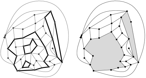
Figure 3: An $O(N)$ configuration on a rooted quadrangulation, with $4$ cycles of total length $30$, and the external gasket associated with this configuration, with shaded holes of degrees $6$ and $14$.

Let $N\geq 0$ be fixed. The annealed $O(N)$ measure is the $\sigma$-finite measure over the set of all pairs $(\mathbf{q},\mathcal{L})$, where $\mathbf{q}$ is a rooted quadrangulation and $\mathcal{L}$ is a loop configuration on $\mathbf{q}$, defined by

$$W_{O(N)}(\mathbf{q},\mathcal{L})=e^{-\beta\#F(\mathbf{q})}x^{\operatorname{lg}(\mathcal{L})}N^{\#\mathcal{L}},$$

where $\beta$ and $x$ are positive parameters. When the total mass $Z_{O(N)}(\beta,x)$ of $W_{O(N)}$ is finite, we say that the pair $(\beta,x)$ is admissible and we can consider the probability measure $P_{O(N)}=Z_{O(N)}(\beta,x)^{-1}W_{O(N)}$.

Consider a configuration $(\mathbf{q},\mathcal{L})$. A cycle $c\in\mathcal{L}$ splits the sphere into two components. The one that contains the face located to the left of the root edge of $\mathbf{q}$ is called the exterior of $c$. The other component is called the interior of $c$. The external gasket $\mathcal{E}(\mathbf{q},\mathcal{L})$ is the rooted planar map obtained from $\mathbf{q}$ by deleting all the edges and vertices strictly contained in the interior of some $c\in\mathcal{L}$; see Figure 3.

More precisely, ${\mathbf{m}}$ is defined as a rooted planar map with two different types of faces:

• faces that came from the exterior of cycles of $\mathcal{L}$, which have degree $4$—we denote by $Q({\mathbf{m}})$ the set of all these faces;

• faces of arbitrary even degree, called the holes of ${\mathbf{m}}$, which came from the deletion of the interior of a cycle of $\mathcal{L}$—we denote by $H({\mathbf{m}})$ the set of all holes of ${\mathbf{m}}$ (note that certain holes may have degree $4$).

Furthermore, the boundaries of the holes of ${\mathbf{m}}$ are disjoint cycles. In particular, every edge of the boundary of a hole is adjacent to a face of $Q({\mathbf{m}})$.

One can verify that the range of the external gasket mapping $(\mathbf{q},\mathcal{L})\to\mathcal{E}(\mathbf{q},\mathcal{L})$ is the set of all rooted planar maps (with faces of two types) satisfying the preceding conditions. It is then an easy exercise to check that the push-forward of $W_{O(N)}$ under the external gasket mapping is

$$W_{O(N)}\bigl{(}\{\mathcal{E}(\mathbf{q},\mathcal{L})={\mathbf{m}}\}\bigr{)}=e^{-\beta\#Q({\mathbf{m}})}\prod_{f\in H({\mathbf{m}})}q_{\deg f/2},$$ (83)

where

$$q_{k}=x^{2k}Z^{\partial}_{O(N),k}(\beta,x)$$

and $Z^{\partial}_{O(N),k}(\beta,x)$ is the partition function for the $O(N)$-model with a boundary of length $2k$. This partition function is defined in an analogous way as $Z_{O(N)}(\beta,x)$, but configurations $(\mathbf{q},\mathcal{L})$ now consist of rooted quadrangulations $\mathbf{q}$ with a boundary of length $2k,$ together with a collection $\mathcal{L}$ of disjoint cycles that do not intersect the boundary and such that the boundary face lies on the left of the root edge. From formula (83), we see that the external gasket of a $P_{O(N)}$-distributed random map has a Boltzmann distribution of a similar kind as those studied in the present work, except that the maps that appear here have two distinct types of faces and extra topological constraints.

Ignoring these extra constraints, one can conjecture that for appropriate values of $\beta$ and $x$, the scaling limits of these random gasket configurations will be closely related to those depicted in Section 7, provided that the weights $q_{k}$ satisfy similar asymptotics as in Section 2.2. At this stage, some predictions from theoretical physics provide insight into these questions. For fixed $\beta$ and $x$, we introduce the generating function

$$Z^{\partial}_{O(N)}(z)=\sum_{k\geq 1}z^{k}Z^{\partial}_{O(N),k}(\beta,x).$$

According to singularity analysis, for $a\in(3/2,2)\cup(2,5/2)$, a behavior

$$Z^{\partial}_{O(N)}(z)\mathop{\approx}_{z\uparrow z_{c}}(z_{c}-z)^{a-1},$$

meaning that the singular part of $Z^{\partial}_{O(N)}$ near its first positive singularity $z_{c}$ is of order $(z_{c}-z)^{a-1}$, leads to asymptotics of the form $Z^{\partial}_{O(N),k}(\beta,x)\sim Ck^{-a}$ for some finite $C>0$; see, for instance, FlSe09 , Corollary VI.1. Of course, this requires additional hypotheses on $Z^{\partial}_{O(N)}(z)$, which we ignore in this informal discussion.

We now summarize, and attempt to translate into a language more familiar to mathematicians, the discussion that can be found in duplantier04 , Appendix B (see, in particular, equations B.48, B.64 and B.78, and the discussion at the end of Section B.1.1 in duplantier04 ). Assume that $N\in(0,2)$ is written in the form $N=2\cos(\pi\theta)$, where $\theta\in(0,1/2)$. One conjectures that there exists a function $x_{c}(\beta)>0$ and a critical value $\beta_{c}>0$ such that:

• for fixed $\beta>\beta_{c}$ and $x=x_{c}(\beta)$,

  $$Z^{\partial}_{O(N)}(z)\mathop{\approx}_{z\uparrow z_{c}}(z_{c}-z)^{1-\theta};$$

• for $\beta=\beta_{c}$ and $x=x_{c}(\beta_{c})$,

  $$Z^{\partial}_{O(N)}(z)\mathop{\approx}_{z\uparrow z_{c}}(z_{c}-z)^{1+\theta}.$$

These two different behaviors, called the dense and the dilute phase, respectively, hint at the asymptotics

$$Z^{\partial}_{O(N),k}(\beta,x)\mathop{\sim}_{k\to\infty}Ck^{-a},$$

with $a=2-\theta$ and $a=2+\theta$, respectively. Recalling Section 2.2 and the preceding formula for $q_{k}$, we see that the scaling limits of the distribution $W_{O(N)}$ in (83) should be related to the model studied in the previous sections, with the particular value $\alpha=a-1/2\in\{3/2-\theta,3/2+\theta\}$. Note that the case $N=2$ appears as a limiting critical situation where the dense and dilute phases should coincide.

A similar description applies to other familiar statistical physics models such as percolation or the Ising model on faces of a random quadrangulation. In the latter setting, a configuration is a pair $(\mathbf{q},\sigma),$ where $\mathbf{q}$ is a rooted quadrangulation and

$$\sigma=\bigl{(}\sigma_{f},f\in F(\mathbf{q})\bigr{)}\in\{-1,+1\}^{F(\mathbf{q})}.$$

In the (annealed) Ising model, one chooses the configuration with probability proportional to

$$W_{I}(\mathbf{q},\sigma)=e^{-\beta\#F(\mathbf{q})}\exp\biggl{(}J\sum_{f\sim f^{\prime}}\sigma_{f}\sigma_{f^{\prime}}\biggr{)},$$

where $J$ is a real parameter and the last sum is over all pairs of adjacent faces $f,f^{\prime}$ in $\mathbf{q}$. For $J=0$, one gets the percolation model, where conditionally on the quadrangulation $\mathbf{q}$, all $\sigma\in\{-1,+1\}^{\#F(\mathbf{q})}$ are equally likely to occur. One then defines the exterior gasket in a way that should be clear from Figure 4. This gasket again has a Boltzmann-type distribution when $(\mathbf{q},\sigma)$ is distributed according to $W_{I}$. As previously, the relevant Boltzmann weights correspond to partition functions for the Ising model on a quadrangulation with a boundary. On the other hand, the topological constraints on the gaskets are now different: the boundaries of holes need not be cycles and do not have to be disjoint (however, an edge can be incident to at most one hole and is incident only once to this hole); see Figure 4.

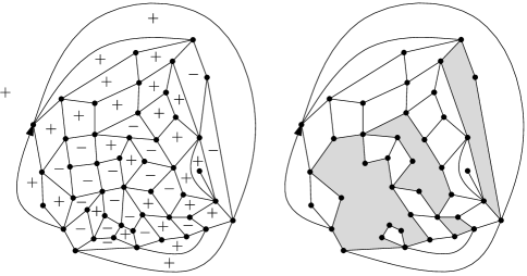
Figure 4: An Ising (or percolation) configuration and the associated exterior gasket.

Kazakov kazakov06 identifies the value $J_{c}=\ln 2$ as critical. One conjectures that, respectively, for $J=J_{c}$ and $0\leq J<J_{c}$ (and with the appropriate values of $\beta$), the Ising model has the same scaling limit as the dilute and dense phases of the $O(N=1)$ model, corresponding to $\theta=1/3$ and $\alpha\in\{11/6,7/6\}$. This is confirmed (for $J=J_{c}$) by predictions for the partition function of the Ising model with a boundary; see, for example, Section 3.3 of COT96 .

Note that a discussion parallel to the present one appears in Sheffield sheffield06 , Section 2.3, in the case of regular hexagonal lattices, where it is conjectured that the external gasket of $O(N)$ models should converge to the so-called conformal loop ensembles, which are a conformally invariant family of random curves related to the Schramm-Loewner evolutions. Such parallel discussions might open some paths in the mathematical understanding of the so-called KPZ formula, which links scaling exponents for models on random and on regular lattices. This approach would still be different from the one developed recently by Duplantier and Sheffield DuSh08 as we are focusing more on the metric aspects of planar maps, rather than on the conformal invariance properties that are intrinsic to DuSh08 .

At a rigorous level, it seems plausible that the topological constraints that appear in the random maps considered above can be handled using bijective methods, in the spirit of Section 3.1. Establishing rigorous grounds for the conjectured behavior of $Z^{\partial}_{O(N)}$ is another, probably much more challenging, problem that would require a better understanding of the combinatorial aspects of the $O(N)$ model on maps.

References

- (1) {bbook}[vtex] \bauthor\bsnmAmbjørn, \bfnmJan\binitsJ., \bauthor\bsnmDurhuus, \bfnmBergfinnur\binitsB. and \bauthor\bsnmJonsson, \bfnmThordur\binitsT. (\byear1997). \btitleQuantum Geometry: A Statistical Field Theory Approach. \bpublisherCambridge Univ. Press, \baddressCambridge. \biddoi=10.1017/CBO9780511524417, mr=1465433 \endbibitem
- (2) {bbook}[mr] \bauthor\bsnmBertoin, \bfnmJean\binitsJ. (\byear1996). \btitleLévy Processes. \bseriesCambridge Tracts in Mathematics \bvolume121. \bpublisherCambridge Univ. Press, \baddressCambridge. \bidmr=1406564 \endbibitem
- (3) {bmisc}[vtex] \bauthor\bsnmBettinelli, \bfnmJ.\binitsJ. (\byear2010). \btitleScaling limits for random quadrangulations of positive genus. Preprint. \bnoteUniv. Paris-Sud. Available at arXiv:1002.3682. \endbibitem
- (4) {barticle}[vtex] \bauthor\bsnmBouttier, \bfnmJ.\binitsJ., \bauthor\bsnmDi Francesco, \bfnmP.\binitsP. and \bauthor\bsnmGuitter, \bfnmE.\binitsE. (\byear2004). \btitlePlanar maps as labeled mobiles. \bjournalElectron. J. Combin. \bvolume11 \bpages27 pp. (electronic). \bidmr=2097335 \endbibitem
- (5) {bbook}[mr] \bauthor\bsnmBurago, \bfnmDmitri\binitsD., \bauthor\bsnmBurago, \bfnmYuri\binitsY. and \bauthor\bsnmIvanov, \bfnmSergei\binitsS. (\byear2001). \btitleA Course in Metric Geometry. \bseriesGraduate Studies in Mathematics \bvolume33. \bpublisherAmer. Math. Soc., \baddressProvidence, RI. \bidmr=1835418 \endbibitem
- (6) {barticle}[vtex] \bauthor\bsnmCarroll, \bfnmSean M.\binitsS. M., \bauthor\bsnmOrtiz, \bfnmMiguel E.\binitsM. E. and \bauthor\bsnmTaylor, \bfnmWashington\binitsW. (\byear1996). \btitleSpin/disorder correlations and duality in the string. \bjournalNuclear Phys. B \bvolume468 \bpages420–438. \biddoi=10.1016/0550-3213(96)00116-2, mr=1399489 \endbibitem
- (7) {barticle}[mr] \bauthor\bsnmChassaing, \bfnmPhilippe\binitsP. and \bauthor\bsnmSchaeffer, \bfnmGilles\binitsG. (\byear2004). \btitleRandom planar lattices and integrated superBrownian excursion. \bjournalProbab. Theory Related Fields \bvolume128 \bpages161–212. \biddoi=10.1007/s00440-003-0297-8, mr=2031225 \endbibitem
- (8) {bbook}[vtex] \bauthor\bsnmDellacherie, \bfnmClaude\binitsC. and \bauthor\bsnmMeyer, \bfnmPaul-André\binitsP.-A. (\byear1980). \btitleProbabilités et Potentiel. Chapitres V à VIII, \beditionRevised ed. \bseriesActualités Scientifiques et Industrielles [Current Scientific and Industrial Topics] \bvolume1385. \bpublisherHermann, \baddressParis. \bidmr=566768 \endbibitem
- (9) {bincollection}[vtex] \bauthor\bsnmDuplantier, \bfnmBertrand\binitsB. (\byear2004). \btitleConformal fractal geometry & boundary quantum gravity. In \bbooktitleFractal Geometry and Applications: A Jubilee of Benoît Mandelbrot, Part 2. \bseriesProceedings of Symposia in Pure Mathematics \bvolume72 \bpages365–482. \bpublisherAmer. Math. Soc., \baddressProvidence, RI. \bidmr=2112128\endbibitem
- (10) {bmisc}[vtex] \bauthor\bsnmDuplantier, \bfnmBertrand\binitsB. and \bauthor\bsnmSheffield, \bfnmS.\binitsS. (\byear2008). \bhowpublishedLiouville quantum gravity and KPZ. Preprint. CEA/Saclay. Available at arXiv:0808.1560. \endbibitem
- (11) {barticle}[vtex] \bauthor\bsnmDuquesne, \bfnmThomas\binitsT. (\byear2003). \btitleA limit theorem for the contour process of conditioned Galton–Watson trees. \bjournalAnn. Probab. \bvolume31 \bpages996–1027. \biddoi=10.1214/aop/1048516543, mr=1964956 \endbibitem
- (12) {barticle}[vtex] \bauthor\bsnmDuquesne, \bfnmThomas\binitsT. and \bauthor\bsnmLe Gall, \bfnmJean-François\binitsJ.-F. (\byear2002). \btitleRandom trees, Lévy processes and spatial branching processes. \bjournalAstérisque \bvolume281 \bpagesvi+147. \bidmr=1954248 \endbibitem
- (13) {bbook}[vtex] \bauthor\bsnmFeller, \bfnmWilliam\binitsW. (\byear1971). \btitleAn Introduction to Probability Theory and Its Applications, \bedition2nd ed. \bpublisherWiley, \baddressNew York. \bidmr=0270403 \endbibitem
- (14) {bbook}[mr] \bauthor\bsnmFlajolet, \bfnmPhilippe\binitsP. and \bauthor\bsnmSedgewick, \bfnmRobert\binitsR. (\byear2009). \btitleAnalytic Combinatorics. \bpublisherCambridge Univ. Press, \baddressCambridge. \bidmr=2483235 \endbibitem
- (15) {bbook}[vtex] \bauthor\bsnmIbragimov, \bfnmI. A.\binitsI. A. and \bauthor\bsnmLinnik, \bfnmYu. V.\binitsY. V. (\byear1971). \btitleIndependent and Stationary Sequences of Random Variables. \bpublisherWolters-Noordhoff, \baddressGroningen. \bidmr=0322926 \endbibitem
- (16) {bbook}[mr] \bauthor\bsnmJacod, \bfnmJean\binitsJ. and \bauthor\bsnmShiryaev, \bfnmAlbert N.\binitsA. N. (\byear1987). \btitleLimit Theorems for Stochastic Processes. \bseriesGrundlehren der Mathematischen Wissenschaften [Fundamental Principles of Mathematical Sciences] \bvolume288. \bpublisherSpringer, \baddressBerlin. \bidmr=959133 \endbibitem
- (17) {barticle}[mr] \bauthor\bsnmKazakov, \bfnmV. A.\binitsV. A. (\byear1986). \btitleIsing model on a dynamical planar random lattice: Exact solution. \bjournalPhys. Lett. A \bvolume119 \bpages140–144. \biddoi=10.1016/0375-9601(86)90433-0, mr=871244 \endbibitem
- (18) {barticle}[mr] \bauthor\bsnmLe Gall, \bfnmJean-François\binitsJ.-F. (\byear2005). \btitleRandom trees and applications. \bjournalProbab. Surv. \bvolume2 \bpages245–311 (electronic). \biddoi=10.1214/154957805100000140, mr=2203728 \endbibitem
- (19) {barticle}[mr] \bauthor\bsnmLe Gall, \bfnmJean-François\binitsJ.-F. (\byear2007). \btitleThe topological structure of scaling limits of large planar maps. \bjournalInvent. Math. \bvolume169 \bpages621–670. \biddoi=10.1007/s00222-007-0059-9, mr=2336042 \endbibitem
- (20) {barticle}[vtex] \bauthor\bsnmLe Gall, \bfnmJ. F.\binitsJ. F. (\byear2010). \btitleGeodesics in large random planar maps and in the Brownian map. \bjournalActa Math. \bnoteTo appear. Available at arXiv:0804.3012. \endbibitem
- (21) {barticle}[mr] \bauthor\bsnmMarckert, \bfnmJean-François\binitsJ.-F. and \bauthor\bsnmMiermont, \bfnmGrégory\binitsG. (\byear2007). \btitleInvariance principles for random bipartite planar maps. \bjournalAnn. Probab. \bvolume35 \bpages1642–1705. \biddoi=10.1214/009117906000000908, mr=2349571 \endbibitem
- (22) {barticle}[mr] \bauthor\bsnmMarckert, \bfnmJean-François\binitsJ.-F. and \bauthor\bsnmMokkadem, \bfnmAbdelkader\binitsA. (\byear2006). \btitleLimit of normalized quadrangulations: The Brownian map. \bjournalAnn. Probab. \bvolume34 \bpages2144–2202. \biddoi=10.1214/009117906000000557, mr=2294979 \endbibitem
- (23) {bincollection}[vtex] \bauthor\bsnmMiermont, \bfnmGrégory\binitsG. (\byear2006). \btitleAn invariance principle for random planar maps. In \bbooktitleFourth Colloquium on Mathematics and Computer Science Algorithms, Trees, Combinatorics and Probabilities. \bpages39–57. \bpublisherAssoc. Discrete Math. Theor. Comput. Sci., \baddressNancy. \bidmr=2509622 \endbibitem
- (24) {barticle}[mr] \bauthor\bsnmMiermont, \bfnmGrégory\binitsG. (\byear2009). \btitleTessellations of random maps of arbitrary genus. \bjournalAnn. Sci. Éc. Norm. Supér. (4) \bvolume42 \bpages725–781. \bidmr=2571957 \endbibitem
- (25) {barticle}[vtex] \bauthor\bsnmMiermont, \bfnmGrégory\binitsG. and \bauthor\bsnmWeill, \bfnmMathilde\binitsM. (\byear2008). \btitleRadius and profile of random planar maps with faces of arbitrary degrees. \bjournalElectron. J. Probab. \bvolume13 \bpages79–106. \bidmr=2375600 \endbibitem
- (26) {bbook}[vtex] \bauthor\bsnmPetrov, \bfnmV. V.\binitsV. V. (\byear1975). \btitleSums of Independent Random Variables. \bpublisherSpringer, \baddressNew York. \bidmr=0388499 \endbibitem
- (27) {bbook}[vtex] \bauthor\bsnmPitman, \bfnmJ.\binitsJ. (\byear2006). \btitleCombinatorial Stochastic Processes. \bseriesLecture Notes in Math. \bvolume1875. \bpublisherSpringer, \baddressBerlin. \bidmr=2245368 \endbibitem
- (28) {barticle}[mr] \bauthor\bsnmSheffield, \bfnmScott\binitsS. (\byear2009). \btitleExploration trees and conformal loop ensembles. \bjournalDuke Math. J. \bvolume147 \bpages79–129. \biddoi=10.1215/00127094-2009-007, mr=2494457 \endbibitem
- (29) {bbook}[vtex] \bauthor\bsnmSpitzer, \bfnmFrank\binitsF. (\byear1976). \btitlePrinciples of Random Walks, \bedition2nd ed. \bseriesGraduate Texts in Mathematics \bvolume34. \bpublisherSpringer, \baddressNew York. \bidmr=0388547 \endbibitem