An Optimal Execution Problem with Market Impact

Abstract

We study an optimal execution problem in a continuous-time market model that considers market impact. We formulate the problem as a stochastic control problem and investigate properties of the corresponding value function. We find that right-continuity at the time origin is associated with the strength of market impact for large sales, otherwise the value function is continuous. Moreover, we show the semi-group property (Bellman principle) and characterise the value function as a viscosity solution of the corresponding Hamilton–Jacobi–Bellman equation. We introduce some examples where the forms of the optimal strategies change completely, depending on the amount of the trader’s security holdings and where optimal strategies in the Black–Scholes type market with nonlinear market impact are not block liquidation but gradual liquidation, even when the trader is risk-neutral.

Keywords: Optimal execution, Market impact, Liquidity problems, Hamilton–Jacobi–Bellman equation (HJB), Viscosity solutions.

1 Introduction

An optimal portfolio management problem was developed in [27], [28] and in other papers. These classical financial theories assumed that assets in the market are perfectly liquid, but real markets pose various liquidity risks. For instance, the problem of transaction costs and the uncertainty of trading.

Another important problem of liquidity is market impact (MI), that is, the effect of trader investment behaviour on security prices. Such problems are often discussed in the framework of optimal execution problems, where a trader holds a certain amount of a security and tries to execute trades within a time horizon. The optimal execution problem considering MI was first studied in [7] as a minimisation problem of an expected execution cost in a discrete-time model, and that model was generalised to a mean-variance model in [4] and [18]. A continuous-time model of the execution problem was studied in [16], [33] and [34] as a singular/impulse stochastic control problem. Forsyth [13] has also studied the continuous-time model in the framework of mean-variance analyses and gave a viscosity characterisation of the corresponding value functions. An infinite time horizon case is treated in [32]. The optimal execution problem in the limit-order-book (LOB) model is studied in [1], [2], [3], [14], [15], [31], etc.

Recently, various studies have examined the optimisation problem with MI, but a standard framework has yet to be established. In this paper we develop a mathematical model of optimal execution. Our model is formulated as a stochastic control problem in the continuous-time model, which is characterised as the limit of those of the discrete-time models (see Section 7).

We study our optimal execution model by investigating the properties of the corresponding value function. First we study the continuity of the value function. We find that our value function is continuous in each parameter except for the time origin, where the right-continuity at $\displaystyle t=0$ is according to the “strength” of MI function. This implies that instantaneous liquidation of large volume makes no sense when MI for large trade is strong (in a meaning to be discussed later). Next we show the semi-group property (the Bellman principle) of the value function. This property is standard in the theory of stochastic control, but a strict proof is generally difficult. We show the semi-group property of our value function by applying an argument based on Nisio’s method ([30]).

The semi-group property suggests that the value function is characterised as a viscosity solution of the corresponding Hamilton–Jacobi–Bellman equation (HJB), which is a nonlinear second order partial differential equation (PDE). We prove that our value function actually becomes a viscosity solution of the HJB, and we also show the uniqueness of viscosity solutions of the HJB under certain mathematical assumptions. Note that the viscosity characterisation of value functions of stochastic control problems has been broadly studied elsewhere ([12], [29] and the references therein). Uniqueness (or the comparison principle) of viscosity solutions of HJB is also well-studied in the theory of nonlinear PDEs (see, for instance, [9], [10]). Nevertheless, our results are original: we cannot apply the existing results to our model because of the unboundedness of the control region and the growth conditions of the coefficients (see Remark 4 for details).

We mainly consider the case where the MI function is convex with respect to execution volume. Although some empirical studies tell us that the MI function becomes concave according to market circumstances (see, for instance, [5]), considering the effect of a convex MI is interesting and important from a theoretical viewpoint. We give some examples that imply that a convex MI function makes a trader avoid a block liquidation (selling all of a security at once) and induce a gradual liquidation (selling over a period of time). As another interesting result, we find that the forms of a risk-neutral trader in the Black–Scholes type model with a (log-)quadratic MI function drastically change according to the initial shares of the security held.

This paper is organised as follows: In Section 2, we introduce our model. In Section 3, we give our main results. We study properties of our value function, namely continuity, the semi-group property and the viscosity characterisation. Moreover, we have the uniqueness result of the viscosity solution of the corresponding HJB when MI is sufficiently strong. In Section 4, we also consider the case where the trader needs to liquidate all holdings of the security. We show that such a ‘sell-off’ (liquidation) condition does not influence the form of the value function in our model. In Section 5, we consider some examples of our model. We summarise this paper in Section 6. In Section 7, we introduce the derivation of our continuous-time model from the discrete-time models, and we give proofs of our results in Section 8.

2 The Model

We now present the details of the model. Let $\displaystyle(\Omega,\mathcal{F},(\mathcal{F}_{t})_{0\leq t\leq T},P)$ be a filtered space that satisfies the usual conditions (i.e., $\displaystyle(\mathcal{F}_{t})_{t}$ is right-continuous and $\displaystyle\mathcal{F}_{0}$ contains all $\displaystyle P$-null sets), and let $\displaystyle(B_{t})_{0\leq t\leq T}$ be a standard one-dimensional $\displaystyle(\mathcal{F}_{t})_{t}$-Brownian motion. Here, $\displaystyle T>0$ denotes the time horizon. For simplicity we assume $\displaystyle T=1$.

Suppose that the market consists of one risk-free asset (cash) and one risky asset (a security). The price of cash is always $\displaystyle 1$, which means that the risk-free rate is zero. The price of the security fluctuates according to a certain stochastic flow, and is influenced by the trader’s sales. We consider a single trader who has an endowment of $\displaystyle\Phi_{0}>0$ shares of a security. This trader liquidates the shares $\displaystyle\Phi_{0}$ over a time interval $\displaystyle[0,1]$, but these sales affect the price of the security.

First, we define trading strategies. We say that a stochastic process $\displaystyle(\zeta_{r})_{0\leq r\leq 1}$ is an admissible execution strategy if $\displaystyle(\zeta_{r})_{r}\in\mathcal{A}_{1}(\Phi_{0})$, where

$$\displaystyle\mathcal{A}_{t}(\varphi) \displaystyle= \displaystyle\Big{\{}(\zeta_{r})_{0\leq r\leq t}\ ;\ (\mathcal{F}_{r})_{r}\mbox{-progressively measurable},\ \ \mbox{nonnegative},$$ (2.1)

$$\displaystyle\hskip 56.9055pt\int^{t}_{0}\zeta_{r}dr\leq\varphi\ \mbox{a.s.},\ \ \sup_{r,\omega}\zeta_{r}(\omega)<\infty\Big{\}}.$$

The value $\displaystyle\zeta_{r}$ represents the instantaneous sales (i.e., execution speed) at time $\displaystyle r$. To avoid technical difficulties, we do not consider short selling in this paper. Thus $\displaystyle\zeta_{r}$ is assumed to be nonnegative. The integral $\displaystyle\int^{t}_{0}\zeta_{r}dr$ denotes the cumulative volume of liquidation until time $\displaystyle t$. The trader cannot liquidate more of the security than the initial shares held. The inequality $\displaystyle\int^{1}_{0}\zeta_{r}dr\leq\Phi_{0}$ represents such a situation. The boundedness $\displaystyle\sup_{r,\omega}\zeta_{r}(\omega)<\infty$ has no financial meaning; the arguments in Section 7 imply that we may consider the continuous-time optimal execution problem in only the case where trading strategies satisfy this condition (see also Remark 1 below).

Next we introduce security price fluctuations and define our MI function. Let $\displaystyle s_{0}>0$ be the initial price and let $\displaystyle x_{0}=\log s_{0}$. $\displaystyle S_{t}$ is the security price at time $\displaystyle t$ and $\displaystyle X_{t}$ is its log-price, so $\displaystyle X_{t}=\log S_{t}$. If the trader does not trade, meaning there is no MI, the fluctuation of $\displaystyle(X_{t})_{t}$ is described by the following stochastic differential equation (SDE):

$$\displaystyle\left\{\begin{array}[]{ll}dX_{r}=\sigma(X_{r})dB_{r}+b(X_{r})dr,&\\ \hskip 5.69054ptX_{0}=x_{0},&\end{array}\right.$$ (2.4)

where $\displaystyle b,\sigma:\mathbb{R}\longrightarrow\mathbb{R}$ are Borel functions. We assume that $\displaystyle b$ and $\displaystyle\sigma$ are bounded and Lipschitz continuous, so there exists a unique solution of (2.4). When the trader liquidates the security with the liquidation schedule $\displaystyle(\zeta_{r})_{r}\in\mathcal{A}_{1}(\Phi_{0})$, the log-price is influenced by MI. In this case $\displaystyle(X_{r})_{r}$ follows

$$\displaystyle\left\{\begin{array}[]{ll}dX_{r}=\sigma(X_{r})dB_{r}+b(X_{r})dr-g(\zeta_{r})dr,&\\ \hskip 5.69054ptX_{0}=x_{0}.&\end{array}\right.$$ (2.7)

Here, $\displaystyle g:[0,\infty)\longrightarrow[0,\infty)$ is our (permanent) MI function, and at time $\displaystyle t$ the log-price decreases by $\displaystyle g(\zeta_{t})dt$ according to the execution speed $\displaystyle\zeta_{t}$. We assume that $\displaystyle g$ is non-decreasing and continuously differentiable; let

$$\displaystyle h(\zeta)=g^{\prime}(\zeta)$$ (2.8)

be its derivative. Then $\displaystyle h$ represents how MI becomes large when the trading size increases. In this paper we consider the case where MI function $\displaystyle g$ is convex (not necessarily strictly convex; $\displaystyle g$ may be assumed to be a linear function); thus $\displaystyle h$ is a non-decreasing function. This assumption is required to show Theorem 1 below. Moreover, the convexity of $\displaystyle g$ plays an essential role in our execution problem, in that this property motivates the trader to liquidate the shares of the security spending time to avoid a huge MI (see Sections 5–6).

Note that the process $\displaystyle(S_{r})_{r}$ satisfies

$$\displaystyle\left\{\begin{array}[]{ll}dS_{r}=\hat{\sigma}(S_{r})dB_{r}+\hat{b}(S_{r})dr-g(\zeta_{r})S_{r}dr,&\\ \hskip 5.69054ptS_{0}=s_{0},&\end{array}\right.$$ (2.11)

where $\displaystyle\hat{\sigma}(s)=s\sigma(\log s)$ and $\displaystyle\hat{b}(s)=s\{b(\log s)+\sigma(\log s)^{2}/2\}$. The existence and uniqueness of solutions of SDEs (2.7)–(2.11) also hold for each admissible strategy $\displaystyle(\zeta_{r})_{r}$.

The trader’s problem is to choose an admissible strategy to maximise the expected utility $\displaystyle\mathop{\rm E}[u(W_{1},\varphi_{1},S_{1})]$ for the utility function $\displaystyle u\in\mathcal{C}$, where $\displaystyle W_{t}$ (resp. $\displaystyle\varphi_{t}$) represents the amount of cash (resp. security) at time $\displaystyle t$, and $\displaystyle\mathcal{C}$ denotes the set of non-decreasing continuous functions on $\displaystyle D=\mathbb{R}\times[0,\Phi_{0}]\times[0,\infty)$ such that

$$\displaystyle u(w,\varphi,s)\leq C_{u}(1+w^{2}+s^{2})^{m_{u}},\ \ (w,\varphi,s)\in D$$ (2.12)

for some constants $\displaystyle C_{u}>0$ and $\displaystyle m_{u}\in\mathbb{N}$ (i.e., $\displaystyle u$ has polynomial growth rate). Mathematically, this problem is characterised by the value function

$$\displaystyle V_{t}(w,\varphi,s;u)=\sup_{(\zeta_{r})_{r}\in\mathcal{A}_{t}(\varphi)}\mathop{\rm E}[u(W_{t},\varphi_{t},S_{t})]$$

subject to

$$\displaystyle(W_{0},\varphi_{0},S_{0})=(w,\varphi,s)$$ (2.13)

and

$$\displaystyle dW_{r} \displaystyle= \displaystyle\zeta_{r}S_{r}dr,$$

$$\displaystyle d\varphi_{r} \displaystyle= \displaystyle-\zeta_{r}dr,$$ (2.14)

$$\displaystyle dS_{r} \displaystyle= \displaystyle\hat{\sigma}(S_{r})dB_{r}+\hat{b}(S_{r})dr-g(\zeta_{r})S_{r}dr$$

for $\displaystyle t\in[0,1],(w,\varphi,s)\in D$, and $\displaystyle u\in\mathcal{C}$. We remark that $\displaystyle V_{0}(w,\varphi,s;u)=u(w,\varphi,s)$. Also note that $\displaystyle V_{t}(w,\varphi,s;u)<\infty$ for any $\displaystyle t\in[0,1]$, $\displaystyle(w,\varphi,s)\in D$ and $\displaystyle u\in\mathcal{C}$ (see Sections 8.1–8.2).

For technical reasons, we allow the security price to take the value $\displaystyle 0$ (note that $\displaystyle\hat{b}(0)$ and $\displaystyle\hat{\sigma}(0)$ are defined as $\displaystyle 0$). When $\displaystyle s>0$, we can obviously rewrite

$$\displaystyle V_{t}(w,\varphi,s;u)=\sup_{(\zeta_{r})_{r}\in\mathcal{A}_{t}(\varphi)}\mathop{\rm E}[u(W_{t},\varphi_{t},S_{t})]$$

subject to (2.13) and

$$\displaystyle dW_{r} \displaystyle= \displaystyle\zeta_{r}\exp(X_{r})dr,$$

$$\displaystyle d\varphi_{r} \displaystyle= \displaystyle-\zeta_{r}dr,$$ (2.15)

$$\displaystyle dX_{r} \displaystyle= \displaystyle\sigma(X_{r})dB_{r}+b(X_{r})dr-g(\zeta_{r})dr,$$

$$\displaystyle S_{r} \displaystyle= \displaystyle\exp(X_{r}).$$

For convenience, we denote a triplet $\displaystyle(W_{r},\varphi_{r},S_{r})_{0\leq r\leq t}$ of (2.13), (2.14) by $\displaystyle\Xi_{t}(w,\varphi,s;\allowbreak(\zeta_{r})_{r})$, and $\displaystyle(W_{r},\varphi_{r},\allowbreak X_{r})_{0\leq r\leq t}$ of (2.13), (2.15) by $\displaystyle\Xi^{X}_{t}(w,\varphi,s;\allowbreak(\zeta_{r})_{r})$.

Note that a trader whose execution strategy is in $\displaystyle\mathcal{A}_{t}(\varphi)$ is permitted to leave shares of the security unsold, and there will be no penalty if the trader cannot finish the liquidation within the time horizon. In Section 4, we consider a case when the trader must finish the liquidation.

Remark 1.

The definition of $\displaystyle V_{t}(w,\varphi,s;u)$ originates from a convergence theorem for value functions of optimal execution problems from discrete-time to continuous-time models. As pointed out in [21], in constructing a mathematical model of a financial problem, the discrete-time model, on the one hand, significantly describes realistic phenomena exactly, but sometimes it is hard to get a clean model due to complex noise. The continuous-time model, on the other hand, often makes problems clear, but the superficial construction of continuous-time models may overlook the essence of the problem. Therefore, it is meaningful to construct an adequate model by the following procedures: we first considered a discrete-time model of an optimal execution problem with MI, and then derived a continuous-time model as the limit. In fact, our value function $\displaystyle V_{t}(w,\varphi,s;u)$ is derived in such a way from given discrete-time models. Please refer to Section 7 for details.

Remark 2.

MI can be divided into two parts: a permanent impact and a temporary impact (see [4] and [17]). As time passes, the temporary impact disappears and the transitorily depressed price recovers. Our MI function $\displaystyle g(\zeta)$ corresponds to the permanent impact.

We can define a value function of the optimal execution problem with both permanent and temporary MI in a continuous-time model such as

$$\displaystyle\hat{V}_{t}(w,\varphi,s;u) \displaystyle= \displaystyle\sup_{(\zeta_{r})_{r}\in\mathcal{A}_{t}(\varphi)}\mathop{\rm E}[u(W_{t},\varphi_{t},S_{t})]$$

$$\displaystyle\mathrm{s.t.} \displaystyle\hskip 0.28453ptdW_{r}=\zeta_{r}\exp(X_{r}-\tilde{g}(\zeta_{r}))dr,$$

$$\displaystyle\hskip 3.69885ptd\varphi_{r}=-\zeta_{r}dr,$$

$$\displaystyle\hskip 2.27621ptdX_{r}=\sigma(X_{r})dB_{r}+b(X_{r})dr-g(\zeta_{r})dr,$$

$$\displaystyle\hskip 9.10486ptS_{r}=\exp(X_{r}),$$

$$\displaystyle(W_{0},\varphi_{0},S_{0})=(w,\varphi,s),$$

where $\displaystyle\tilde{g}(\zeta)$ denotes the temporary MI function. We can also show continuity of this value function in $\displaystyle w,\varphi$ and $\displaystyle s$. However, constructing a discrete-time version of the problem is difficult due to technical reasons. Moreover, the Bellman principle (Theorem 2 in the next section) is proved by Nisio’s method, which is based on a discrete-time approximation of the value function. Since Theorem 2 plays an essential role in proving Theorem 1 (especially continuity in $\displaystyle t$) and Theorems 3 and 4, we cannot sufficiently study the properties of our value function when there is temporary MI. In this paper, therefore, we treat only permanent MI functions. For further comments, see Section 6.

3 Main Results

Next we present the main results of this paper. First we introduce the result of the continuity of $\displaystyle V_{t}(w,\varphi,s;u)$. Here we denote $\displaystyle h(\infty)=\lim_{\zeta\rightarrow\infty}h(\zeta)$ for brevity.

Theorem 1.

Let $\displaystyle u\in\mathcal{C}$.
$\displaystyle\mathrm{(i)}$  If $\displaystyle h(\infty)=\infty$, then $\displaystyle V_{t}(w,\varphi,s;u)$ is continuous in $\displaystyle(t,w,\varphi,s)\in[0,1]\times D$.
$\displaystyle\mathrm{(ii)}$  If $\displaystyle h(\infty)<\infty$, then $\displaystyle V_{t}(w,\varphi,s;u)$ is continuous in $\displaystyle(t,w,\varphi,s)\in(0,1]\times D$ and $\displaystyle V_{t}(w,\varphi,s;u)$ converges to $\displaystyle Ju(w,\varphi,s)$ uniformly on any compact subset of $\displaystyle D$ as $\displaystyle t\downarrow 0$, where

$$\displaystyle Ju(w,\varphi,s)=\left\{\begin{array}[]{ll}\sup_{\psi\in[0,\varphi]}u\Big{(}w+\frac{1-e^{-h(\infty)\psi}}{h(\infty)}s,\varphi-\psi,se^{-h(\infty)\psi}\Big{)}&(h(\infty)>0)\\ \sup_{\psi\in[0,\varphi]}u(w+\psi s,\varphi-\psi,s)&(h(\infty)=0).\end{array}\right.$$

We prove Theorem 1 in Section 8.4. As we can see, continuity in $\displaystyle t$ at the origin depends on the state of the function $\displaystyle h$ at infinity. When $\displaystyle h(\infty)=\infty$, MI of large sales is strong enough ($\displaystyle g(\zeta)$ diverges rapidly with $\displaystyle\zeta\rightarrow\infty$) to make a trader avoid instantaneous liquidation. An optimal policy is ‘no-trading’ in an infinitesimal time; thus, $\displaystyle V_{t}$ converges to $\displaystyle u$ as $\displaystyle t\downarrow 0$. When $\displaystyle h(\infty)<\infty$, the value function is not always continuous at $\displaystyle t=0$ and has the right limit $\displaystyle Ju(w,\varphi,s)$. In this case, MI for large sales is not as strong ($\displaystyle g(\zeta)$ diverges, but the divergence speed is slow) and there is room for successful liquidation in the infinitesimal time. The function $\displaystyle Ju(w,\varphi,s)$ corresponds to the utility of liquidation by a trader who sells a part of the shares of a security $\displaystyle\psi$ by dividing infinitely within an infinitely short time (such that the fluctuation of the security price is negligible) and who is left with the amount $\displaystyle\varphi-\psi$, that is,

$$\displaystyle\zeta^{\delta}_{r}=\frac{\psi}{\delta}1_{[0,\delta]}(r),\ \ r\in[0,t]\ \ (\delta\downarrow 0).$$ (3.2)

Such a strategy is also discussed in [26]. We remark that the form of $\displaystyle Ju$ is strongly related to Theorem 3 in [26] (see Theorem 2 in Section 4 for more details). Also note that the condition $\displaystyle h(\infty)=0$ corresponds to the classical case of no MI model.

Next we study the semi-group property (the Bellman principle) of the family of nonlinear operators corresponding with the continuous-time value function. We define an operator $\displaystyle Q_{t}:\mathcal{C}\longrightarrow\mathcal{C}$ by $\displaystyle Q_{t}u(w,\varphi,s)=V_{t}(w,\varphi,s;u)$. Here the arguments in Sections 8.1–8.2 imply that $\displaystyle Q_{t}$ is well-defined. We now have the following theorem.

Theorem 2.

For each $\displaystyle r,t\in[0,1]$ with $\displaystyle t+r\leq 1$,  $\displaystyle(w,\varphi,s)\in D$ and $\displaystyle u\in\mathcal{C}$ it holds that $\displaystyle Q_{t+r}u(w,\varphi,s)=Q_{t}Q_{r}u(w,\varphi,s)$.

The proof is given in Section 8.3. Using Theorem 2, we can characterise the continuous-time value function as the viscosity solution of the corresponding HJB. Since the value functions are defined in a way that does not depend on $\displaystyle\Phi_{0}$, we can take them to be defined on an extended domain $\displaystyle\hat{D}=\mathbb{R}\times[0,\infty)\times[0,\infty)$. Let $\displaystyle u(w,\varphi,s):\hat{D}\longrightarrow\mathbb{R}$ be such that $\displaystyle u$ is a non-decreasing continuous function that grows polynomially in $\displaystyle w,\varphi$ and $\displaystyle s$. We define a function $\displaystyle F:\mathscr{S}\longrightarrow[-\infty,\infty)$ by

$$\displaystyle F(z,p,X)=-\sup_{\zeta\geq 0}\left\{\frac{1}{2}\hat{\sigma}(z_{s})^{2}X_{ss}+\hat{b}(z_{s})p_{s}+\zeta\left(z_{s}p_{w}-p_{\varphi}\right)-g(\zeta)z_{s}p_{s}\right\},$$

where $\displaystyle\mathscr{S}=\hat{U}\times\mathbb{R}^{3}\times S^{3}$, $\displaystyle\hat{U}=\hat{D}\setminus\partial\hat{D}$, $\displaystyle S^{3}$ is the space of symmetric matrices in $\displaystyle\mathbb{R}^{3}\otimes\mathbb{R}^{3}$, and

$$\displaystyle z=\left(\begin{array}[]{c}z_{w}\\ z_{\varphi}\\ z_{s}\end{array}\right)\in D,\ p=\left(\begin{array}[]{c}p_{w}\\ p_{\varphi}\\ p_{s}\end{array}\right)\in\mathbb{R}^{3},\ X=\left(\begin{array}[]{ccc}X_{ww}&X_{w\varphi}&X_{ws}\\ X_{\varphi w}&X_{\varphi\varphi}&X_{\varphi s}\\ X_{sw}&X_{s\varphi}&X_{ss}\end{array}\right)\in S^{3}.$$

Although the function $\displaystyle F$ approach $\displaystyle-\infty$, we can define a viscosity solution of the following HJB as usual (see, e.g., [12], [23] and [29]):

$$\displaystyle\frac{\partial}{\partial t}v+F(z,\mathcal{D}v,\mathcal{D}^{2}v)=0\ \ \mathrm{on}\ (0,1]\times\hat{U},$$ (3.4)

where $\displaystyle\mathcal{D}$ denotes the differential operator with respect to $\displaystyle z=(w,\varphi,s)$. Here, we remark that $\displaystyle(\ref{HJB2})$ can be rewritten as

$$\displaystyle\frac{\partial}{\partial t}v(t,w,\varphi,s)-\sup_{\zeta\geq 0}\mathscr{L}^{\zeta}v(t,w,\varphi,s)=0,\ \ (t,w,\varphi,s)\in(0,1]\times\hat{U},$$ (3.5)

where

$$\displaystyle\mathscr{L}^{\zeta}v(t,w,\varphi,s)=\frac{1}{2}\hat{\sigma}(s)^{2}\frac{\partial^{2}}{\partial s^{2}}v(t,w,\varphi,s)+\hat{b}(s)\frac{\partial}{\partial s}v(t,w,\varphi,s)$$

$$\displaystyle\hskip 56.9055pt+\zeta\Big{(}s\frac{\partial}{\partial w}v(t,w,\varphi,s)-\frac{\partial}{\partial\varphi}v(t,w,\varphi,s)\Big{)}-g(\zeta)s\frac{\partial}{\partial s}v(t,w,\varphi,s).$$

Now we state the following theorem, which is proved in Section 8.6.

Theorem 3.

Assume that $\displaystyle h$ is strictly increasing and $\displaystyle h(\infty)=\infty$. Moreover, assume

$$\displaystyle\liminf_{\varepsilon\downarrow 0}\frac{V_{t}(w,\varphi,s+\varepsilon;u)-V_{t}(w,\varphi,s;u)}{\varepsilon}>0$$ (3.6)

for any $\displaystyle t\in(0,1]$ and $\displaystyle(w,\varphi,s)\in\hat{U}$. Then $\displaystyle V_{t}(w,\varphi,s;u)$ is a viscosity solution of $\displaystyle(\ref{HJB2})$.

This theorem tells us that when $\displaystyle h(\infty)=\infty$ (MI is strong), our value function is characterised by the corresponding HJB (3.4).

Remark 3.

It is quite natural that the value function is increasing with respect to the underlying security price, and we can easily prove that $\displaystyle V_{t}(w,\varphi,s;u)$ is non-decreasing in $\displaystyle s$. Then it follows that

$$\displaystyle\liminf_{\varepsilon\downarrow 0}\frac{V_{t}(w,\varphi,s+\varepsilon;u)-V_{t}(w,\varphi,s;u)}{\varepsilon}\geq 0.$$

The inequality (3.6) is stricter than the one above, and is needed to prove our characterisation result (Theorem 3) because of technical reasons related to when $\displaystyle F=-\infty$ occurs. Note also that in many cases we may easily show that the value function is strictly increasing in $\displaystyle s$, that is, $\displaystyle V_{t}(w,\varphi,s+\varepsilon;u)-V_{t}(w,\varphi,s;u)>0$ for $\displaystyle\varepsilon>0$. Nevertheless, this does not directly indicate (3.6). Here, we present a sufficient condition for (3.6).

• $\displaystyle u(w,\varphi,s)=U(w)$ for some $\displaystyle U\in C^{1}(\mathbb{R})$. Moreover, $\displaystyle U$ is concave and $\displaystyle U^{\prime}(w)\geq\delta$,  $\displaystyle w\in\mathbb{R}$ for some $\displaystyle\delta>0$.

• Coefficients $\displaystyle b$ and $\displaystyle\sigma$ in (2.7) are differentiable and their derivatives are Lipschitz continuous and uniformly bounded.

Then we can show the following proposition:

Proposition 1.

Assume $\displaystyle[C1]$–$\displaystyle[C2]$. Then the inequality $\displaystyle(\ref{cond_diff})$ holds.

The proof is in Section 8.5. Note that the conditions [C1]–[C2] are satisfied in typical cases. [C1] corresponds to the risk-averse (or risk-neutral) trader, which is standard in finance. [C1] further requires that the utility function depends only on the cash holdings $\displaystyle w$, but this assumption is also mild and standard (especially when we consider the sell-off condition, which will be discussed in Section 4). [C2] is satisfied in typical cases, such as the Black–Scholes model: In Section 5, we will treat such an example when the trader is risk-neutral.

Finally, we give the uniqueness result of viscosity solutions of (3.5).

Theorem 4.

Assume that $\displaystyle\hat{\sigma}$ and $\displaystyle\hat{b}$ are both Lipschitz continuous. Assume the hypotheses of Theorem 3 and that $\displaystyle\liminf_{\zeta\rightarrow\infty}(h(\zeta)/\zeta)>0$. If a polynomial growth function $\displaystyle v:[0,1]\times\hat{D}\longrightarrow\mathbb{R}$ is a viscosity solution of $\displaystyle(\ref{HJB})$ and satisfies the boundary conditions

$$\displaystyle\begin{array}[]{rl}v(0,w,\varphi,s)=u(w,\varphi,s),&(w,\varphi,s)\in\hat{D},\\ v(t,w,0,s)=\mathrm{E}\left[u\left(w,0,Z_{t}(s)\right)\right],&(t,w,s)\in[0,1]\times\mathbb{R}\times[0,\infty),\\ v(t,w,\varphi,0)=u(w,\varphi,0),&(t,w,\varphi)\in[0,1]\times\mathbb{R}\times[0,\infty),\end{array}$$ (3.10)

then $\displaystyle V_{t}(w,\varphi,s;u)=v(t,w,\varphi,s)$, where

$$\displaystyle Z_{t}(s)=\exp\left(Y_{t}(\log s)\right)\ (s>0),\ \ 0\ (s=0)$$ (3.11)

and $\displaystyle Y_{t}(x)$ is the solution of SDE $\displaystyle(\ref{SDE_X0})$ replacing $\displaystyle x_{0}$ with $\displaystyle x$, that is, where $\displaystyle Z_{t}(s)$ represents the price of the security with no MI.

The proof of Theorem 4 is given in Section 8.7. This theorem guarantees the uniqueness of viscosity solutions of (3.5) when the divergence speed of $\displaystyle g(\zeta)$ with $\displaystyle\zeta\rightarrow\infty$ is greater than or equal to a quadratic function, that is, when $\displaystyle g(\zeta)\geq C\zeta^{2}$, $\displaystyle\zeta\geq M$ for some $\displaystyle C,M>0$. In Section 5.2, we present an example where the assumptions in Theorems 3 and 4 are fulfilled.

Remark 4.

Characterisation of value functions of a stochastic control problem as viscosity solutions of HJB has been discussed in many papers and textbooks (e.g., [9], [10], [12] and [29]). Uniqueness results of viscosity solutions of HJB are also well studied. Yet to the best of our knowledge, the characterisation theorem (Theorem 3) and the uniqueness theorem (Theorem 4) of our HJB (3.4) cannot be derived from the existing literature. The main difficulties are as follows:

• Our control region $\displaystyle[0,\infty)$ is unbounded.

• The drift term $\displaystyle\hat{b}(s)-g(\zeta)s$ does not always satisfy the linear growth condition in $\displaystyle s$ and $\displaystyle\zeta$. In particular, if $\displaystyle h(\infty)=\infty$, then we never get the estimates

  $$\displaystyle|g(\zeta)s|\leq C(1+\zeta+s),\ \ |g(\zeta)s-g(\zeta)s^{\prime}|\leq C(1+\zeta)|s-s^{\prime}|,\ \ s,s^{\prime},\zeta\geq 0$$

  for any positive constant $\displaystyle C$.

Recently, the uniqueness of viscosity solutions of HJB has been studied for unbounded domains (in our case, $\displaystyle\hat{D}=\mathbb{R}\times[0,\infty)\times[0,\infty)$) and unbounded control regions (in our case, $\displaystyle[0,\infty)$). Theorem 2.1 of [10] is one of the most general results of the comparison principle of viscosity solutions of HJB. However, our HJB does not satisfy conditions (A)(ii)–(iii) in [10]. Thus, we cannot apply those results, meaning that our results are original in this respect.

4 Sell-Off Condition

In this section we consider the optimal execution problem under the ‘sell-off condition’. A trader has a certain quantity of shares of a security at some initial time, and must liquidate all of them within a time horizon. Then the spaces of admissible strategies are reduced to

$$\displaystyle\mathcal{A}^{\mathrm{SO}}_{t}(\varphi)=\left\{(\zeta_{r})_{r}\in\mathcal{A}_{t}(\varphi)\ ;\ \int^{t}_{0}\zeta_{r}dr=\varphi\right\}.$$

We define a value function with the sell-off condition by

$$\displaystyle V^{\mathrm{SO}}_{t}(w,\varphi,s;U)=\sup_{(\zeta_{r})_{r}\in\mathcal{A}^{\mathrm{SO}}_{t}(\varphi)}\mathop{\rm E}[U(W_{t})]$$

subject to (2.13)–(2.14) for a continuous, non-decreasing, polynomially growing function $\displaystyle U:\mathbb{R}\longrightarrow\mathbb{R}$. This gives the following theorem:

Theorem 1.

$\displaystyle V^{\mathrm{SO}}_{t}(w,\varphi,s;U)=V_{t}(w,\varphi,s;u)$, where $\displaystyle u(w,\varphi,s)=U(w)$.

Proof.

The relation $\displaystyle V^{\mathrm{SO}}_{t}(w,\varphi,s;U)\leq V_{t}(w,\varphi,s;u)$ is trivial, so we will show only the assertion $\displaystyle V^{\mathrm{SO}}_{t}(w,\varphi,s;U)\geq V_{t}(w,\varphi,s;u)$. Take any $\displaystyle(\zeta_{r})_{r}\in\mathcal{A}_{t}(\varphi)$ and let $\displaystyle(W_{r},\varphi_{r},S_{r})_{r}=\Xi_{1}(w,\varphi,s;(\zeta_{r})_{r})$. Moreover take any $\displaystyle\delta\in(0,t)$. We define an execution strategy $\displaystyle(\zeta^{\delta}_{r})_{r}\in\mathcal{A}^{\mathrm{SO}}_{t}(\varphi)$ by $\displaystyle\zeta^{\delta}_{r}=\zeta_{r}\ (r\in[0,t-\delta]),\ \ \varphi_{t-\delta}/\delta\ (r\in(t-\delta,t])$. Let $\displaystyle(W^{\delta}_{r},\varphi^{\delta}_{r},S^{\delta}_{r})_{r}=\Xi_{1}(w,\varphi,s;(\zeta^{\delta}_{r})_{r})$. Then we have $\displaystyle W_{t-\delta}=W^{\delta}_{t-\delta}\leq W^{\delta}_{t}$. Thus we get $\displaystyle\mathop{\rm E}[U(W_{t-\delta})]\leq\mathop{\rm E}[U(W^{\delta}_{t})]\leq V^{\mathrm{SO}}_{t}(w,\varphi,s;U)$. Letting $\displaystyle\delta\downarrow 0$, we have $\displaystyle\mathop{\rm E}[U(W_{t})]\leq V^{\mathrm{SO}}_{t}(w,\varphi,s;U)$ by the monotone convergence theorem (note that $\displaystyle U(W_{t-\delta})\geq U(w)>-\infty$). Since $\displaystyle(\zeta_{r})_{r}\in\mathcal{A}_{t}(\varphi)$ is arbitrary, we obtain the assertion. ∎

By Theorem 1, we see that the sell-off condition $\displaystyle\int^{t}_{0}\zeta_{r}dr=\varphi$ makes no change in the (value of the) value function. No such phenomenon is observed in a discrete-time framework; although the value function in a discrete-time model in Section 7 may depend on whether the sell-off condition is imposed, in the continuous-time model we need not worry about such a condition.

When $\displaystyle g(\zeta)$ is linear, we can apply the variable reduction method ($\displaystyle 9^{\prime}$)–($\displaystyle 12^{\prime}$) in [26] to obtain the following:

Theorem 2.

Assume $\displaystyle g(\zeta)=\alpha\zeta$ for $\displaystyle\alpha>0$.
$\displaystyle\mathrm{(i)}$  $\displaystyle V^{\mathrm{SO}}_{t}(w,\varphi,s;U)=\overline{V}^{\varphi}_{t}\left(w+\frac{1-e^{-\alpha\varphi}}{\alpha}s,e^{-\alpha\varphi}s;U\right)$, where

$$\displaystyle\overline{V}^{\varphi}_{t}(\bar{w},\bar{s};U) \displaystyle= \displaystyle\sup_{(\bar{\varphi}_{r})_{r}\in\overline{\mathcal{A}}_{t}(\varphi)}\mathop{\rm E}[U(\bar{W}_{t})]$$

$$\displaystyle\hskip 19.91692pt\mathrm{s.t.}\hskip 17.92523ptd\bar{S}_{r}=e^{-\alpha\bar{\varphi}_{r}}\hat{b}(\bar{S}_{r}e^{\alpha\bar{\varphi}_{r}})dr+e^{-\alpha\bar{\varphi}_{r}}\hat{\sigma}(\bar{S}_{r}e^{\alpha\bar{\varphi}_{r}})dB_{r},$$

$$\displaystyle\hskip 48.36967ptd\bar{W}_{r}=\frac{e^{\alpha\bar{\varphi}_{r}}-1}{\alpha}d\bar{S}_{r},$$

$$\displaystyle\hskip 56.9055pt\bar{S}_{0}=\bar{s},\ \ \bar{W}_{0}=\bar{w},$$

and

$$\displaystyle\overline{\mathcal{A}}_{t}(\varphi)=\left\{\left(\varphi-\int^{r}_{0}\zeta_{v}dv\right)_{0\leq r\leq t}\ ;\ (\zeta_{r})_{0\leq r\leq t}\in\mathcal{A}^{\mathrm{SO}}_{t}(\varphi)\right\}.$$

$\displaystyle\mathrm{(ii)}$  If $\displaystyle U$ is concave and $\displaystyle\hat{b}\leq 0$, then

$$\displaystyle V^{\mathrm{SO}}_{t}(w,\varphi,s;U)=U\left(w+\frac{1-e^{-\alpha\varphi}}{\alpha}s\right).$$ (4.1)

A proof is given in Section 8.10. Note that assertion (ii) is the same as Theorem 3 in [26], and in this case we can get the explicit form of the value function. The right side of (4.1) equals $\displaystyle Ju(w,\varphi,s)$ for $\displaystyle u(w,\varphi,s)=U(w)$ and the nearly optimal strategy for $\displaystyle V^{\mathrm{SO}}_{t}(w,\varphi,s;U)=V_{t}(w,\varphi,s;u)$ is given by (3.2).

5 Examples

In this section, we consider two examples of our model. Let $\displaystyle b(x)\equiv-\mu$ and $\displaystyle\sigma(x)\equiv\sigma$ for some constants $\displaystyle\mu,\sigma\geq 0$ and suppose $\displaystyle\tilde{\mu}=\mu-\sigma^{2}/2>0$. We assume that the trader has a risk-neutral utility function $\displaystyle u(w,\varphi,s)=u_{\mathrm{RN}}(w,\varphi,s)=w$. Note that we can replace the stochastic control problem $\displaystyle V_{t}(w,\varphi,s;u_{\mathrm{RN}})$ with the deterministic control problem $\displaystyle f(t,\varphi)$, where

$$\displaystyle f(t,\varphi) \displaystyle= \displaystyle\sup_{(\zeta_{r})_{r}\in\mathcal{A}^{\mathrm{det}}_{t}(\varphi)}\tilde{f}(t,\varphi;(\zeta_{r})_{r}),$$

$$\displaystyle\tilde{f}(t,\varphi;(\zeta_{r})_{r}) \displaystyle= \displaystyle\int^{t}_{0}\zeta_{r}\exp\left(-\tilde{\mu}r-\int^{r}_{0}g(\zeta_{v})dv\right)dr,$$

$$\displaystyle\mathcal{A}^{\mathrm{det}}_{t}(\varphi) \displaystyle= \displaystyle\{(\zeta_{r})_{r}\in\mathcal{A}_{t}(\varphi)\ ;\ (\zeta_{r})_{r}\mathrm{\ is\ deterministic}\}.$$

Indeed,

Proposition 2.

$\displaystyle V_{t}(w,\varphi,s;u_{\mathrm{RN}})=w+sf(t,\varphi)$.

This is proved in Section 8.9. By Proposition 2, we see that

$$\displaystyle\frac{\partial}{\partial s}V_{t}(w,\varphi,s;u_{\mathrm{RN}})=f(t,\varphi)>0,\ \ t,\varphi>0,$$

which implies (3.6).

5.1 Log-Linear Impact

Set $\displaystyle g(\zeta)=\alpha\zeta$ for $\displaystyle\alpha>0$. The following theorem is a direct consequence of Theorem 2(ii).

Theorem 1.

It holds that

$$\displaystyle V_{t}(w,\varphi,s;u_{\mathrm{RN}})=w+\frac{1-e^{-\alpha\varphi}}{\alpha}s$$ (5.1)

for all $\displaystyle t\in(0,1]$ and $\displaystyle(w,\varphi,s)\in D$.

The right side of (5.1) converges to $\displaystyle w+\varphi s$ as $\displaystyle\alpha\downarrow 0$, which is the profit gained by choosing the so-called block liquidation execution strategy, that is, by a trader selling all shares $\displaystyle\varphi$ at $\displaystyle t=0$ when there is no MI. Theorem 1 implies that the optimal strategy in this case is to liquidate all shares, dividing infinitely within an infinitely short time at $\displaystyle t=0$. This is almost the same as a block liquidation at the initial time, and the trader does not delay the execution time (although MI lowers the profit from the liquidation). Therefore, we cannot see any essential influence of the MI in this example.

Remark 5.

We can also obtain the (nearly) optimal strategies in the cases of $\displaystyle\tilde{\mu}<0$ and $\displaystyle\tilde{\mu}=0$. When $\displaystyle\tilde{\mu}<0$, the nearly optimal strategy is the (almost) block liquidation at the terminal time. When $\displaystyle\tilde{{\mu}}=0$, each strategy in $\displaystyle\mathcal{A}^{\mathrm{SO}}_{t}(\varphi)$ makes the same profit: in other words, all the strategies in $\displaystyle\mathcal{A}^{\mathrm{SO}}_{t}(\varphi)$ are optimal.

5.2 Log-Quadratic Impact

In this subsection we consider the case of a strictly convex MI function. Set $\displaystyle g(\zeta)=\alpha\zeta^{2}$ for $\displaystyle\alpha>0$. Note that $\displaystyle h(\zeta)/\zeta=2\alpha>0$, and thus the value function in this example is the unique viscosity solution of (3.4) with boundary conditions (3.10), by Theorems 3 and 4.

As we will see, we can derive the explicit form of an optimal strategy when $\displaystyle\varphi$ is sufficiently small or large. However, when $\displaystyle\varphi$ is not sufficiently small, such a strategy has unbounded execution speed and is not subject to $\displaystyle\mathcal{A}_{t}(\varphi)$. Thus we extend the set of admissible strategies:

$$\displaystyle\tilde{\mathcal{A}}_{t}(\varphi) \displaystyle= \displaystyle\big{\{}(\zeta_{r})_{0\leq r\leq t}\ ;\ (\mathcal{F}_{r})_{r}\mbox{-adapted},\ \zeta_{r}\geq 0,\ \int^{t}_{0}\zeta_{r}dr\leq\varphi$$

$$\displaystyle\hskip 65.44133pt\mathrm{and}\ \sup_{(r,\omega)\in[0,t-\varepsilon]\times\Omega}\zeta_{r}(\omega)<\infty\ \mathrm{for\ all}\ \varepsilon\in(0,t)\big{\}},$$

$$\displaystyle\tilde{\mathcal{A}}^{\mathrm{det}}_{t}(\varphi) \displaystyle= \displaystyle\{(\zeta_{r})_{r}\in\tilde{\mathcal{A}}_{t}(\varphi)\ ;\ (\zeta_{r})_{r}\mathrm{\ is\ deterministic}\}$$

to allow unbounded execution speed at $\displaystyle t$. We can see that the value of $\displaystyle f(t,\varphi)$ does not change by replacing $\displaystyle\mathcal{A}^{\mathrm{det}}_{t}(\varphi)$ with $\displaystyle\tilde{\mathcal{A}}^{\mathrm{det}}_{t}(\varphi)$. Indeed, for each $\displaystyle(\zeta_{r})_{r}\in\tilde{\mathcal{A}}^{\mathrm{det}}_{t}(\varphi)$, the integrability of $\displaystyle\zeta_{r}$ on $\displaystyle[0,t]$ $\displaystyle\left(\mathrm{i.e.}\int^{t}_{0}\zeta_{r}dr\leq\varphi<\infty\right)$, the dominated convergence theorem, and the continuity of $\displaystyle f(t,\varphi)$ in $\displaystyle t$ (this is obtained by Theorem 1(i) and Proposition 2) imply

$$\displaystyle\tilde{f}(t,\varphi;(\zeta_{r})_{r}) \displaystyle= \displaystyle\lim_{\varepsilon\rightarrow 0}\tilde{f}(t-\varepsilon,\varphi;(\zeta_{r})_{r})$$ (5.2)

$$\displaystyle\leq \displaystyle\lim_{\varepsilon\rightarrow 0}f(t-\varepsilon,\varphi)=f(t,\varphi).$$

So we get

$$\displaystyle f(t,\varphi)=\sup_{(\zeta_{r})_{r}\in\tilde{\mathcal{A}}^{\mathrm{det}}_{t}(\varphi)}\tilde{f}(t,\varphi;(\zeta_{r})_{r}).$$

Thus, we can also restrict the set of admissible strategies of $\displaystyle V_{t}(w,\varphi,s;\allowbreak u_{\mathrm{R}N})$ to $\displaystyle\tilde{\mathcal{A}}^{\mathrm{det}}_{t}(\varphi)$ by Proposition 2.

We define the functions $\displaystyle\hat{v}^{i}(t,w,\varphi,s)$ and $\displaystyle\hat{\zeta}^{i}_{r}$, $\displaystyle i=1,2$, by

$$\displaystyle\hat{v}^{1}(t,w,\varphi,s)=w+\frac{s\sqrt{1-e^{-2\tilde{\mu}t}}}{2\sqrt{\alpha\tilde{\mu}}},\ \ \hat{\zeta}^{1}_{r}=\sqrt{\frac{\tilde{\mu}}{\alpha(1-e^{-2\tilde{\mu}(t-r)})}}$$

and

$$\displaystyle\hat{v}^{2}(t,w,\varphi,s)=w+\frac{s}{2\sqrt{\alpha\tilde{\mu}}}(1-e^{-2\sqrt{\alpha\tilde{\mu}}\varphi}),\ \ \hat{\zeta}^{2}_{r}=\sqrt{\frac{\tilde{\mu}}{\alpha}}1_{[0,\varphi\sqrt{\alpha/\tilde{\mu}}]}(r).$$

Moreover we set

$$\displaystyle\hat{\Phi}^{1}(t)=\frac{\mathrm{arctanh}\sqrt{1-e^{-2\tilde{\mu}t}}}{\sqrt{\alpha\tilde{\mu}}},\ \ \hat{\Phi}^{2}(t)=\sqrt{\frac{\tilde{\mu}}{\alpha}}t.$$ (5.3)

Then we have the following theorem:

Theorem 2.

$\displaystyle(\mathrm{i})$  If $\displaystyle\varphi\geq\hat{\Phi}^{1}(t)$, then $\displaystyle V_{t}(w,\varphi,s;u_{\mathrm{RN}})=\hat{v}^{1}(t,w,\varphi,s)$ and $\displaystyle(\hat{\zeta}^{1}_{r})_{r}$ is an optimal strategy.
$\displaystyle(\mathrm{ii})$  If $\displaystyle\varphi\leq\hat{\Phi}^{2}(t)$, then $\displaystyle V_{t}(w,\varphi,s;u_{\mathrm{RN}})=\hat{v}^{2}(t,w,\varphi,s)$ and $\displaystyle(\hat{\zeta}^{2}_{r})_{r}$ is an optimal strategy.

Proof.

Let $\displaystyle(\hat{W}^{i}_{r},\hat{\varphi}^{i}_{r},\hat{S}^{i}_{r})_{r}=\Xi_{t}(w,\varphi,s;(\hat{\zeta}^{i}_{r})_{r})$ for $\displaystyle i=1,2$. Straightforward calculation shows that $\displaystyle\mathop{\rm E}[\hat{W}^{i}_{t}]=\hat{v}^{i}(t,w,\varphi,s)$. Then we have $\displaystyle\hat{v}^{i}(t,w,\varphi,s)\leq V_{t}(w,\varphi,s;u_{\mathrm{RN}})$. Since $\displaystyle\hat{v}^{i}$ satisfies (3.5) at $\displaystyle(t,w,\varphi,s)$, we see that $\displaystyle\hat{v}^{i}(t,w,\varphi,s)\geq V_{t}(w,\varphi,s;\allowbreak u_{\mathrm{RN}})$ by Theorem 5.2.1 in [29], thus fulfilling the assertion. ∎

This theorem implies that the form of optimal strategies and value functions varies, depending on the amount of the security holdings $\displaystyle\varphi$. If a trader has a small amount of securities, then we have case (ii) and the optimal strategy is to sell the entire holdings until the time $\displaystyle\varphi\sqrt{\alpha/\tilde{\mu}}$. If a trader has a large amount, then we have case (i) and the trader cannot finish the selling.

We do not have an explicit form for $\displaystyle V_{t}(w,\varphi,s;u_{\mathrm{RN}})$ on the whole space, so we try to solve this example numerically. By Proposition 2, it suffices to consider the numerical calculation of $\displaystyle f(t,\varphi)$. Moreover, $\displaystyle f(t,\varphi)$ is approximated by $\displaystyle f^{n}_{[nt]}(\varphi)$ with large $\displaystyle n$, where

$$\displaystyle f^{n}_{k}(\varphi) \displaystyle= \displaystyle\sup_{(\psi^{n}_{l})_{l}\in\mathcal{A}^{n,\mathrm{det}}(\varphi)}\sum^{k-1}_{l=0}\psi^{n}_{l}\exp\left(-\tilde{\mu}\times\frac{l}{n}-n\alpha\sum^{l}_{m=0}(\psi^{n}_{m})^{2}\right),$$ (5.4)

$$\displaystyle\mathcal{A}^{n,\mathrm{det}}_{k}(\varphi) \displaystyle= \displaystyle\left\{(\psi^{n}_{l})^{k-1}_{l=0}\subset[0,\varphi]^{k}\ ;\ \sum^{k-1}_{l=0}\psi^{n}_{l}\leq\varphi\right\}.$$ (5.5)

In fact, the convergence of $\displaystyle f^{n}_{[nt]}$ to $\displaystyle f_{t}$ is given by the same proof as Theorem 1 in Section 7. $\displaystyle f^{n}_{k}(\varphi)$ corresponds to a nonlinear optimisation problem with $\displaystyle k$ variables. We solve it numerically by the sequential quadratic programming method.

It can be numerically verified that the convergence of $\displaystyle f^{n}_{[nt]}$ takes place before $\displaystyle n=500$. Thus, we set $\displaystyle n=500$ below and we regard $\displaystyle f^{500}_{[500t]}(\varphi)$ as a precise approximation of $\displaystyle f(t,\varphi)$. We set other parameters as $\displaystyle w=0,s=1,\alpha=0.01$, and $\displaystyle\tilde{\mu}=0.05$.

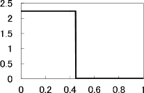
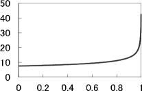
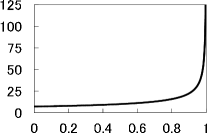
Figure 1: The forms of optimal execution strategies $\displaystyle(\zeta_{r})_{r}$. Horizontal axis is time $\displaystyle r$. Left: $\displaystyle\varphi=1$. Centre: $\displaystyle\varphi=10$. Right: $\displaystyle\varphi=100$. In the centre graph, $\displaystyle(\zeta_{r})_{r}$ was calculated numerically.

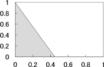
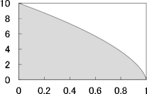
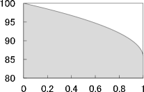
Figure 2: The forms of the amount of security holdings $\displaystyle(\varphi_{r})_{r}$ corresponding to optimal strategies. Horizontal axis is time $\displaystyle r$. Left: $\displaystyle\varphi=1$. Centre: $\displaystyle\varphi=10$. Right: $\displaystyle\varphi=100$. In the centre graph, $\displaystyle(\varphi_{r})_{r}$ was calculated numerically.

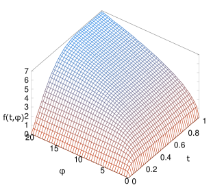
Figure 3: The form of the function $\displaystyle f(t,\varphi)$.

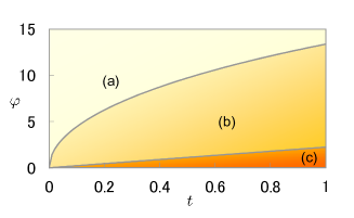
Figure 4: The region of pairs $\displaystyle(t,\varphi)$. The region (a) (resp. (c)) corresponds to Theorem 2 (i) (resp. (ii)).

Figure 1 describes the form of the execution strategies and Figure 2 describes the form of the corresponding processes of the amount of a security with $\displaystyle\varphi=1,10$, and $\displaystyle 100$. We also get the form of the function $\displaystyle f(t,\varphi)$ of Proposition 2 numerically, as described in Figure 4. If a pair $\displaystyle(t,\varphi)$ is in the range (a) of Figure 4, then we have $\displaystyle f(t,\varphi)=\sqrt{1-e^{-2\tilde{\mu}t}}/(2\sqrt{\alpha\tilde{\mu}})$, and if $\displaystyle(t,\varphi)$ is in the range (c), we have $\displaystyle f(t,\varphi)=(1-e^{-2\sqrt{\alpha\tilde{\mu}}\varphi})/(2\sqrt{\alpha\tilde{\mu}})$. We have not had the form of $\displaystyle f(t,\varphi)$ analytically when $\displaystyle(t,\varphi)$ is in the range (b).

Note that in case (i) we can also construct a nearly optimal strategy with the sell-off condition. Let $\displaystyle\hat{\zeta}^{1,\delta}_{r}=\hat{\zeta}^{1}_{r}\ (r\leq t-\delta),\ (\varphi-\hat{\varphi}_{t-\delta})/\delta\ (t-\delta<r\leq t)$, where

$$\displaystyle\hat{\varphi}_{t-\delta}=\frac{\mathrm{arctanh}\sqrt{1-e^{-2\tilde{\mu t}}}-\mathrm{arctanh}\sqrt{1-e^{-2\tilde{\mu}\delta}}}{\sqrt{\alpha\tilde{\mu}}}.$$

Then $\displaystyle(\hat{\zeta}^{1,\delta}_{r})_{r}\in\mathcal{A}^{\mathrm{SO}}_{t}(\varphi)$ and the corresponding expected profit $\displaystyle\mathop{\rm E}[\hat{W}^{\delta}_{t}]$ converges to $\displaystyle V_{t}(w,\varphi,s;u_{\mathrm{RN}})$ as $\displaystyle\delta\rightarrow 0$.

6 Concluding Remarks

In this paper we studied the optimal execution problem when MI is considered. We mainly considered the case where the MI function is convex. This was done for both mathematical and financial reasons. In a Black–Scholes type market, the optimal execution strategy of a risk-neutral trader is block liquidation when there is no MI. As we saw in Section 5, the form of the optimal strategy changes when MI is log-quadratic. In contrast, when MI is not convex, and especially when it is log-linear, the trader’s optimal strategy is almost block liquidation.

In the real market, however, many traders take their time selling, despite recognition that the MI is concave. One reason may be that the trader has a risk-averse utility function. We surmise another reason: the existence of a temporary (or transient) impact (see Remark 2). Our examples treat only permanent impact, but we can also consider the case where MI disappears as time passes by price recovery effects: if the process of security prices follows some mean-reverting process, such as an Ornstein–Uhlenbeck process, then we may deal with the optimisation problem with MI and price recovery. We study such a case in [22].

It is also meaningful to characterise the value function as the solution of the corresponding HJB. We have shown that the value function is a viscosity solution under some strong assumptions. Such assumptions would not be necessary if we considered only bounded strategies, but the control region of our model is unbounded. We avoid this difficulty by supposing (3.6) which is satisfied in financially natural settings.

In trading operations, the trader should execute trades while considering fluctuations of the price of other assets (e.g., rebalancing an index fund). In [19], a multidimensional version of this model was studied to consider such a case. However, in the case of rebalancing, it is necessary to consider not only selling securities but also buying them. We should carefully formulate models of optimal execution so that no trader gets a free lunch when MI is large.

The complete solution of our example in Section 5.2 is another remaining task. This is a representative example where a trading policy is strongly influenced by MI, and it would be interesting to solve this completely in future research.

7 Appendix A: Derivation of the Continuous-Time Model from the Discrete-Time Models

Here we construct a discrete-time model of an optimal execution with time interval $\displaystyle 1/n$ ($\displaystyle n=1,2,3,\ldots$). As in Section 2, we prepare a filtered space $\displaystyle(\Omega,\mathcal{F},(\mathcal{F}_{t})_{0\leq t\leq 1},\allowbreak P)$ satisfying the usual condition and a one-dimensional $\displaystyle(\mathcal{F}_{t})_{t}$-Brownian motion $\displaystyle(B_{t})_{t}$. We assume that there are cash and a security and that the risk-free rate is equal to zero (i.e., the price of cash is $\displaystyle 1$). We consider a single trader who has $\displaystyle\varphi$ shares of the security at the initial time and tries to sell them.

Now we consider the situation of trading at each execution time $\displaystyle t=0,1/n,\allowbreak 2/n,\ldots,$ and describe the effect of the trader’s liquidation. For $\displaystyle l=0,\ldots,n$, we denote by $\displaystyle S^{n}_{l}$ the price of the security at time $\displaystyle l/n$ and $\displaystyle X^{n}_{l}=\log S^{n}_{l}$. Let $\displaystyle s>0$ be the initial price (i.e., $\displaystyle S^{n}_{0}=s$) and $\displaystyle X^{n}_{0}=\log s$. If the trader sells $\displaystyle\psi^{n}_{l}$ at time $\displaystyle l/n$, the log-price changes to $\displaystyle X^{n}_{l}-g_{n}(\psi^{n}_{l})$, where $\displaystyle g_{n}:[0,\infty)\longrightarrow[0,\infty)$ is a non-decreasing and continuously differentiable function which satisfies $\displaystyle g_{n}(0)=0$. The function $\displaystyle g_{n}$ denotes the MI function in the discrete-time model: $\displaystyle g_{n}(\psi^{n}_{l})$ implies the impact of the liquidation of $\displaystyle\psi^{n}_{l}$ shares for the log-price of the security. So the security price $\displaystyle S^{n}_{l}$ decreases to $\displaystyle S^{n}_{l}\exp(-g_{n}(\psi^{n}_{l}))$ by the liquidation. Then the trader gets $\displaystyle\psi^{n}_{l}S^{n}_{l}\exp(-g_{n}(\psi^{n}_{l}))$ in cash as the proceeds of the liquidation. Thus, if we denote by $\displaystyle W^{n}_{l}$ (resp. $\displaystyle\varphi^{n}_{l}$) the amount of the cash holdings (resp. security holdings), then we have the following relations

$$\displaystyle W^{n}_{l+1}=W^{n}_{l}+\psi^{n}_{l}S^{n}_{l}\exp(-g_{n}(\psi^{n}_{l})),\ \ \varphi^{n}_{l+1}=\varphi^{n}_{l}-\psi^{n}_{l}.$$ (7.1)

The former means the increase of the cash holdings and the latter means the decrease of the security holdings.

After trading at time $\displaystyle l/n$, $\displaystyle X^{n}_{l+1}$ and $\displaystyle S^{n}_{l+1}$ are given by

$$\displaystyle X^{n}_{l+1}=Y\Big{(}\frac{l+1}{n};\frac{l}{n},X^{n}_{l}-g_{n}(\psi^{n}_{l})\Big{)},\ \ S^{n}_{l+1}=\exp(X^{n}_{l+1}),$$ (7.2)

where $\displaystyle Y(t;r,y)$ is the solution of the SDE

$$\displaystyle\left\{\begin{array}[]{ll}dY(t;r,y)=\sigma(Y(t;r,y))dB_{t}+b(Y(t;r,y))dt,&t\geq r,\\ \hskip 5.69054ptY(r;r,y)=y.&\end{array}\right.$$ (7.5)

Note that if the trader makes no liquidation, then the unaffected log-price $\displaystyle X^{n}_{l}$ coincides with $\displaystyle Y(l/n;0,x)$. The first equation of (7.2) describes the fluctuation of the log-price as time passes from $\displaystyle l/n$ (with the affected log-price $\displaystyle X^{n}_{l}-g_{n}(\psi^{n}_{l})$) to $\displaystyle(l+1)/n$.

Here we give a class of our execution strategies. Let $\displaystyle\mathcal{A}^{n}_{k}(\varphi)$ be the set of strategies $\displaystyle(\psi^{n}_{l})^{k-1}_{l=0}$ such that $\displaystyle\psi^{n}_{l}$ is $\displaystyle\mathcal{F}_{l/n}$-measurable, $\displaystyle\psi^{n}_{l}\geq 0$ for any $\displaystyle l=0,\ldots,k-1$, and $\displaystyle\sum^{k-1}_{l=0}\psi^{n}_{l}\leq\varphi$. We call $\displaystyle\mathcal{A}^{n}_{k}(\varphi)$ the set of admissible strategies. An admissible strategy is the sequence of random variables (liquidation volumes) $\displaystyle(\psi^{n}_{l})_{l}$ which are constructed by only selling with short-sale constraint (the trader does not buy and does not sell short).

At the end of the time interval $\displaystyle[0,1]$ (i.e. $\displaystyle 1=n/n$), the trader has the amount of cash $\displaystyle W^{n}_{n}$ and the amount of the security $\displaystyle\varphi^{n}_{n}$, which are determined by (7.1) for each $\displaystyle l=0,\ldots,n-1$ and initial values $\displaystyle W^{n}_{0}=w,\ \varphi^{n}_{0}=\varphi$.

Now we define our value function in the discrete-time model. For $\displaystyle(w,\varphi,s)\in D$, $\displaystyle k=0,\ldots,n$ and $\displaystyle u\in\mathcal{C}$ (the definitions of $\displaystyle D$ and $\displaystyle\mathcal{C}$ are the same as Section 2), set

$$\displaystyle V^{n}_{k}(w,\varphi,s;u)=\sup_{(\psi^{n}_{l})^{k-1}_{l=0}\in\mathcal{A}^{n}_{k}(\varphi)}\mathop{\rm E}[u(W^{n}_{k},\varphi^{n}_{k},S^{n}_{k})],$$ (7.6)

subject to (7.1) and (7.2) for $\displaystyle l=0,\ldots,k-1$ and $\displaystyle(W^{n}_{0},\varphi^{n}_{0},S^{n}_{0})=(w,\varphi,s)$ when $\displaystyle s>0$. In the case of $\displaystyle s=0$, we define $\displaystyle V^{n}_{k}(w,\varphi,0;u)=u(w,\varphi,0)$.

Now we assume condition [A]:
[A]  $\displaystyle\lim_{n\rightarrow\infty}\sup_{\psi\in[0,\Phi_{0}]}\Big{|}\frac{d}{d\psi}g_{n}(\psi)-h(n\psi)\Big{|}=0$.

Recall that $\displaystyle h(\zeta)=g^{\prime}(\zeta)$ is a non-negative, non-decreasing, and continuous function (see Section 2). Under condition [A], we see that $\displaystyle\varepsilon_{n}\longrightarrow 0$, where

$$\displaystyle\varepsilon_{n}=\sup_{\psi\in(0,\Phi_{0}]}\Big{|}\frac{g_{n}(\psi)}{\psi}-\frac{g(n\psi)}{n\psi}\Big{|}.$$ (7.7)

This implies the relation between the MI function in the discrete-time model and the one in the continuous-time model. The condition [A] roughly means the $\displaystyle C^{1}$-convergence of $\displaystyle g_{n}$ to $\displaystyle g$. Under [A], we can prove the following theorem.

Theorem 1.

For any $\displaystyle(w,\varphi,s)\in D$, $\displaystyle t\in[0,1]$ and $\displaystyle u\in\mathcal{C}$,

$$\displaystyle\lim_{n\rightarrow\infty}V^{n}_{[nt]}(w,\varphi,s;u)=V_{t}(w,\varphi,s;u),$$ (7.8)

where $\displaystyle[nt]$ is the greatest integer less than or equal to $\displaystyle nt$.

A proof is given in Section 8.8. Theorem 1 implies the convergence of the discrete-time value function to the continuous-time one. In other words, our model in Section 2 is characterised as the limit of the discrete-time models.

8 Appendix B: Proofs

8.1 Preliminaries

We introduce some lemmas used to prove our main results.

Lemma 1.

For any $\displaystyle m\in\mathbb{N}$ there is a constant $\displaystyle C>0$ depending only on $\displaystyle b,\sigma$ and $\displaystyle m$ such that $\displaystyle\mathop{\rm E}[\hat{Z}(s)^{m}]\leq Cs^{m}$, where $\displaystyle\hat{Z}(s)=\sup_{0\leq t\leq 1}Z_{t}(s)$ and $\displaystyle Z_{t}(s)$ is defined in Theorem 4.

Proof.

We may assume $\displaystyle s>0$. By the definition of $\displaystyle\hat{Z}(s)$, we have

$$\displaystyle\mathop{\rm E}[\hat{Z}(s)^{m}]\leq s^{m}\mathop{\rm E}[\sup_{t\in[0,1]}\tilde{Z}_{t}],$$

where $\displaystyle(\tilde{Z}_{t})_{t}$ is given by $\displaystyle\tilde{Z}_{0}=1$ and

$$\displaystyle d\tilde{Z}_{t}=m\tilde{Z}_{t}\sigma\left(\frac{1}{m}\log\tilde{Z}_{t}\right)dB_{t}+m\tilde{Z}_{t}\left\{b\left(\frac{1}{m}\log\tilde{Z}_{t}\right)+\frac{m}{2}\sigma\left(\frac{1}{m}\log\tilde{Z}_{t}\right)^{2}\right\}dt.$$

Using Corollary 2.5.10 in [24] for the process $\displaystyle(\tilde{Z}_{t})_{t}$, we have the assertion. ∎

Lemma 2.

Let $\displaystyle\Gamma_{k}$, $\displaystyle k\in\mathbb{N}$, be sets, $\displaystyle u\in\mathcal{C}$ and let $\displaystyle(W^{i}_{k,\gamma},\varphi^{i}_{k,\gamma},S^{i}_{k,\gamma})\in D$, $\displaystyle\gamma\in\Gamma_{k}$, $\displaystyle k\in\mathbb{N}$, $\displaystyle i=1,2$, be random variables. Let $\displaystyle m_{u}\in\mathbb{N}$ be as in $\displaystyle(\ref{growth_C})$. Suppose

$$\displaystyle\lim_{k\rightarrow\infty}\sup_{\gamma\in\Gamma_{k}}\mathop{\rm E}[|W^{1}_{k,\gamma}-W^{2}_{k,\gamma}|+|\varphi^{1}_{k,\gamma}-\varphi^{2}_{k,\gamma}|+|S^{1}_{k,\gamma}-S^{2}_{k,\gamma}|]=0$$

and $\displaystyle\sum^{2}_{i=1}\sup_{k\in\mathbb{N}}\sup_{\gamma\in\Gamma_{k}}\mathop{\rm E}[(W^{i}_{k,\gamma})^{4m_{u}}+(S^{i}_{k,\gamma})^{4m_{u}}]<\infty$. Then

$$\displaystyle\lim_{k\rightarrow\infty}\sup_{\gamma\in\Gamma_{k}}\big{|}\mathop{\rm E}[u(W^{1}_{k,\gamma},\varphi^{1}_{k,\gamma},S^{1}_{k,\gamma})]-\mathop{\rm E}[u(W^{2}_{k,\gamma},\varphi^{2}_{k,\gamma},S^{2}_{k,\gamma})]\big{|}=0.$$

This lemma is obtained by standard arguments using the Chebyshev inequality and the uniform continuity of $\displaystyle u(w,\varphi,s)$ on $\displaystyle D_{R}$ for any $\displaystyle R>0$, where $\displaystyle D_{R}=[-R,R]\times[0,\Phi_{0}]\times[0,R]$.

Using the Burkholder–Davis–Gundy inequality and the Hölder inequality, we have the following lemma:

Lemma 3.

Let $\displaystyle t\in[0,1]$, $\displaystyle\varphi\geq 0$, $\displaystyle x\in\mathbb{R}$, $\displaystyle(\zeta_{r})_{0\leq r\leq t}\in\mathcal{A}_{t}(\varphi)$ and let $\displaystyle(X_{r})_{0\leq r\leq t}$ be given by $\displaystyle(\ref{SDE_X})$ with $\displaystyle X_{0}=x$. Then there is a constant $\displaystyle C>0$ depending only on $\displaystyle b$ and $\displaystyle\sigma$, such that

$$\displaystyle\mathop{\rm E}\Big{[}\sup_{r\in[r_{0},r_{1}]}\Big{|}X_{r}-X_{r_{0}}+\int^{r}_{r_{0}}g(\zeta_{v})dv\Big{|}^{4}\Big{]}\leq C(r_{1}-r_{0})^{2},\ \ 0\leq r_{0}\leq r_{1}\leq t.$$

Lemma 4.

Let $\displaystyle t\in[0,1]$, $\displaystyle\varphi\geq 0$, $\displaystyle x\in\mathbb{R}$, $\displaystyle(\zeta_{r})_{0\leq r\leq t},(\zeta^{\prime}_{r})_{0\leq r\leq t}\in\mathcal{A}_{t}(\varphi)$ and suppose $\displaystyle(X_{r})_{0\leq r\leq t}$ $\displaystyle($resp., $\displaystyle(X^{\prime}_{r})_{0\leq r\leq t}$$\displaystyle)$ is given by $\displaystyle(\ref{SDE_X})$ with $\displaystyle(\zeta_{r})_{r}$ $\displaystyle($resp., $\displaystyle(\zeta^{\prime}_{r})_{r}$$\displaystyle)$ and $\displaystyle X_{0}=x\leq X^{\prime}_{0}$. Suppose $\displaystyle\zeta_{r}\leq\zeta^{\prime}_{r}$ for any $\displaystyle r\in[0,t]$ almost surely. Then $\displaystyle X_{r}\geq X^{\prime}_{r}$ for any $\displaystyle r\in[0,t]$ almost surely. In particular, we have $\displaystyle\exp(X_{r})\leq\hat{Z}(e^{x})$.

This lemma is obtained by the same arguments as in the proof of Proposition 5.2.18 in [20]. Lemmas 1 and 4 imply

Lemma 5.

For $\displaystyle t\in[0,1]$ and $\displaystyle u\in\mathcal{C}$, $\displaystyle V_{t}(w,\varphi,s;u)$ is non-decreasing in $\displaystyle w,\varphi$ and $\displaystyle s$, and has polynomial growth rate with respect to $\displaystyle w$ and $\displaystyle s$.

8.2 Strategy-Restricted Value Functions

We prepare strategy-restricted value functions to prove Theorems 1 and 2. For $\displaystyle L>0$, we define

$$\displaystyle\mathcal{A}^{L}_{t}(\varphi) \displaystyle= \displaystyle\{(\zeta_{r})_{0\leq r\leq t}\in\mathcal{A}_{t}(\varphi)\ ;\ \sup_{r,\omega}|\zeta_{r}(\omega)|\leq L\},$$

$$\displaystyle V^{L}_{t}(w,\varphi,s;u) \displaystyle= \displaystyle\sup_{(\zeta_{r})_{r\leq t}\in\mathcal{A}^{L}_{t}(\varphi)}\mathop{\rm E}[u(W_{t},\varphi_{t},S_{t})].$$

We easily see that $\displaystyle V_{t}(w,\varphi,s;u)=\sup_{L>0}\allowbreak V^{L}_{t}(w,\varphi,s;u)$.

Now we consider the continuity of $\displaystyle V^{L}_{t}(w,\varphi,s;u)$. Our purpose here is to prove the following proposition:

Proposition 3.

$\displaystyle V^{L}_{t}(w,\varphi,s;u)$ is continuous with respect to $\displaystyle(t,w,\varphi,s)\in[0,1]\times D$.

To prove Proposition 3, we prove the following lemmas:

Lemma 6.

For any $\displaystyle(w,\varphi,s)\in D$ and $\displaystyle t\in[0,1]$

$$\displaystyle\lim_{(w^{\prime},\varphi^{\prime},s^{\prime})\rightarrow(w,\varphi,s)}\sup_{L>0}|V^{L}_{t}(w^{\prime},\varphi^{\prime},s^{\prime};u)-V^{L}_{t}(w,\varphi,s;u)|=0.$$

Proof.

Let $\displaystyle R>0$ and $\displaystyle(w,\varphi,s),(w^{\prime},\varphi^{\prime},s^{\prime})\in D_{R}$. We may assume $\displaystyle s^{\prime}>0$. Take any $\displaystyle(\zeta_{r})_{r\leq t}\in\mathcal{A}^{L}_{t}(\varphi)$. Let $\displaystyle\rho=\inf\{r>0\ ;\ \int^{r}_{0}\zeta_{v}dv>\varphi\wedge\varphi^{\prime}\}\wedge t$ and $\displaystyle\zeta^{\prime}_{r}=\zeta_{r}1_{\{r\leq\rho\}}$. Then $\displaystyle(\zeta^{\prime}_{r})_{r\leq t}\in\mathcal{A}^{L}_{t}(\varphi^{\prime})$. Let $\displaystyle(W_{r},\varphi_{r},S_{r})_{r\leq t}=\Xi_{t}(w,\varphi,s;(\zeta_{r})_{r})$ and $\displaystyle(W^{\prime}_{r},\varphi^{\prime}_{r},S^{\prime}_{r})_{r\leq t}=\Xi_{t}(w^{\prime},\varphi^{\prime},s^{\prime};(\zeta^{\prime}_{r})_{r})$. Moreover, let us define $\displaystyle(\tilde{S}^{\prime}_{r})_{r\leq t}$ by

$$\displaystyle d\tilde{S}^{\prime}_{r}=\hat{\sigma}(\tilde{S}^{\prime}_{r})dB_{r}+\hat{b}(\tilde{S}^{\prime}_{r})dr-g(\zeta_{r})\tilde{S}^{\prime}_{r}dr,\ \ \tilde{S}^{\prime}_{0}=s^{\prime}.$$

Then Lemma 4 implies $\displaystyle S^{\prime}_{r}\geq\tilde{S}^{\prime}_{r}$ for any $\displaystyle r\in[0,t]$ almost surely. Thus

$$\displaystyle\mathop{\rm E}[u(W_{t},\varphi_{t},S_{t})]-V_{t}(w^{\prime},\varphi^{\prime},s^{\prime};u)\leq\mathop{\rm E}[|u(W_{t},\varphi_{t},S_{t})-u(W^{\prime}_{t},\varphi^{\prime}_{t},\tilde{S}^{\prime}_{t})|].\hskip 14.22636pt$$ (8.1)

By a simple calculation we get

$$\displaystyle|W_{t}-W^{\prime}_{t}|\leq|w-w^{\prime}|+\hat{Z}(s)|\varphi-\varphi^{\prime}|+\Phi_{0}\sup_{r\in[0,t]}|S_{r}-\tilde{S}^{\prime}_{r}|$$

and $\displaystyle|\varphi_{t}-\varphi^{\prime}_{t}|\leq|\varphi-\varphi^{\prime}|$. Moreover, Theorem 3.2.7 in [29] and Lemma 1 imply

$$\displaystyle\mathop{\rm E}[\sup_{r\in[0,t]}|S_{r}-\tilde{S}^{\prime}_{r}|]\leq\left\{\begin{array}[]{ll}C_{0}s^{\prime}&(s=0)\\ C_{0}|\log s-\log s^{\prime}|&(s>0)\end{array}\right.$$

for some $\displaystyle C_{0}>0$ depending on only $\displaystyle b,\sigma$ and $\displaystyle R$. Then we obtain

$$\displaystyle\sup_{L>0}\sup_{(\zeta_{r})_{r}\in\mathcal{A}^{L}_{t}(\varphi)}\mathop{\rm E}[|u(W_{t},\varphi_{t},S_{t})-u(W^{\prime}_{t},\varphi^{\prime}_{t},\tilde{S}^{\prime}_{t})|]\longrightarrow 0$$ (8.3)

as $\displaystyle(w^{\prime},\varphi^{\prime},s^{\prime})\rightarrow(w,\varphi,s)$ by Lemma 2. Now (8.1) and (8.3) imply

$$\displaystyle\lim_{(w^{\prime},\varphi^{\prime},s^{\prime})\rightarrow(w,\varphi,s)}\sup_{L>0}(V^{L}_{t}(w,\varphi,s;u)-V^{L}_{t}(w^{\prime},\varphi^{\prime},s^{\prime};u))\leq 0.$$

A similar argument gives us

$$\displaystyle\lim_{(w^{\prime},\varphi^{\prime},s^{\prime})\rightarrow(w,\varphi,s)}\sup_{L>0}(V^{L}_{t}(w^{\prime},\varphi^{\prime},s^{\prime};u)-V^{L}_{t}(w,\varphi,s;u))\leq 0.$$

This establishes the assertion. ∎

Lemma 7.

For any compact set $\displaystyle E\subset D$,

$$\displaystyle\limsup_{r\uparrow t}\sup_{L>0}\sup_{(w,\varphi,s)\in E}(V^{L}_{r}(w,\varphi,s;u)-V^{L}_{t}(w,\varphi,s;u))\leq 0,\ \ t\in(0,1],$$

$$\displaystyle\limsup_{t\downarrow r}\sup_{L>0}\sup_{(w,\varphi,s)\in E}(V^{L}_{r}(w,\varphi,s;u)-V^{L}_{t}(w,\varphi,s;u))\leq 0,\ \ r\in[0,1).$$

Proof.

Let $\displaystyle r,t\in[0,1]$ with $\displaystyle r<t$. Lemmas 2 and 3 imply

$$\displaystyle\sup_{L>0}\sup_{(w,\varphi,s)\in E}\sup_{(\zeta_{v})_{v}\in\mathcal{A}^{L}_{r}(\varphi)}\mathop{\rm E}[|u(W_{r},\varphi_{r},\exp(X_{r}))]-u(\tilde{W}_{t},\tilde{\varphi}_{t},\exp(\tilde{X}_{t}))|]\longrightarrow 0$$

as $\displaystyle r\uparrow t$ and $\displaystyle t\downarrow r$, where $\displaystyle(W_{v},\varphi_{v},X_{v})_{v}=\Xi^{X}_{r}(w,\varphi,s;(\zeta_{v})_{v})$, $\displaystyle(\tilde{W}_{v},\tilde{\varphi}_{v},\tilde{X}_{v})_{v}=\Xi^{X}_{t}(w,\varphi,s;(\tilde{\zeta}_{v})_{v})$ and $\displaystyle\tilde{\zeta}_{v}=\zeta_{v}1_{[0,r]}(v)$ for $\displaystyle(\zeta_{r})_{r}\in\mathcal{A}^{L}_{t}(\varphi)$. This implies the assertions. ∎

Similar arguments give us the following lemma:

Lemma 8.

For any $\displaystyle L>0$ and compact set $\displaystyle E\subset D$,

$$\displaystyle\limsup_{r\uparrow t}\sup_{(w,\varphi,s)\in E}(V^{L}_{t}(w,\varphi,s;u)-V^{L}_{r}(w,\varphi,s;u))\leq 0,\ \ t\in(0,1],$$

$$\displaystyle\limsup_{t\downarrow r}\sup_{(w,\varphi,s)\in E}(V^{L}_{t}(w,\varphi,s;u)-V^{L}_{r}(w,\varphi,s;u))\leq 0,\ \ r\in[0,1).$$

By Lemmas 6–8, we obtain Proposition 3. We remark that Lemma 5 and Proposition 3 imply $\displaystyle V^{L}_{t}(\cdot;u),V_{t}(\cdot;u)\in\mathcal{C}$.

We introduce a version of Theorem 1, which will be used to prove Theorem 2 in the next section. Set

$$\displaystyle\mathcal{A}^{n,L}_{k}(\varphi) \displaystyle= \displaystyle\{(\psi_{l})^{k-1}_{l=0}\in\mathcal{A}^{n}_{k}(\varphi)\ ;\ \psi_{l}\leq L/n,\ l=0,\ldots,k-1\},$$

$$\displaystyle V^{n,L}_{k}(w,\varphi,s;u) \displaystyle= \displaystyle\sup_{(\psi_{l})^{k-1}_{l=0}\in\mathcal{A}^{n,L}_{k}(\varphi)}\mathop{\rm E}[u(W^{n}_{k},\varphi^{n}_{k},S^{n}_{k})].$$

Note that $\displaystyle V^{n}_{k}(w,\varphi,s;u)=\sup_{L>0}V^{n,L}_{k}(w,\varphi,s;u)$. By similar arguments as in Section 8.8, we see that

Proposition 4.

For any $\displaystyle L>0$, $\displaystyle t\in[0,1]$ and $\displaystyle u\in\mathcal{C}$, the convergence

$$\displaystyle\lim_{n\rightarrow\infty}V^{n,L}_{[nt]}(w,\varphi,s;u)=V^{L}_{t}(w,\varphi,s;u).$$

holds uniformly on any compact subset of $\displaystyle D$.

8.3 Proof of Theorem 2

We apply Nisio’s method ([30]) to show Theorem 2. We define the operators $\displaystyle Q^{L}_{t}:\mathcal{C}\longrightarrow\mathcal{C}$ and $\displaystyle Q^{n,L}_{t}:\mathcal{C}\longrightarrow\mathcal{C}$ by $\displaystyle Q^{L}_{t}u(w,\varphi,s)=V^{L}_{t}(w,\varphi,s;u)$ and $\displaystyle Q^{n,L}_{t}u(w,\varphi,s)=V^{2^{n},L}_{[2^{n}t]}(w,\varphi,s;u)$. We see that $\displaystyle Q^{L}_{t}$ and $\displaystyle Q^{n,L}_{t}$ are well defined by the results in Section 8.2 and the standard arguments of discrete-time dynamic programming theory (see [6] for instance). First we show

$$\displaystyle Q^{L}_{t+r}u(w,\varphi,s)=Q^{L}_{t}Q^{L}_{r}u(w,\varphi,s)$$ (8.4)

for any $\displaystyle t,r\in I$ with $\displaystyle t+r\leq 1$, where $\displaystyle I=\{k/2^{l}\ ;\ k,l\in\mathbb{Z}_{+}\}\cap[0,1]$. Let $\displaystyle n\in\mathbb{N}$ be large enough so that $\displaystyle 2^{n}t,2^{n}r\in\mathbb{Z}_{+}$. By the Bellman equation of the discrete-time case ([6]), we have

$$\displaystyle Q^{n,L}_{t+r}u(w,\varphi,s)=Q^{n,L}_{t}Q^{n,L}_{r}u(w,\varphi,s).$$ (8.5)

By Proposition 4, we see that the left side of (8.5) converges to that of (8.4) as $\displaystyle n\rightarrow\infty$ for any $\displaystyle t,r\in I$. The following proposition will give the convergence of the right side.

Proposition 5.

Let $\displaystyle u_{n},u\in\mathcal{C}$ be utility functions satisfying $\displaystyle(\ref{growth_C})$ for some $\displaystyle C_{u}$ and $\displaystyle m_{u}$. Assume that $\displaystyle u_{n}$ converges to $\displaystyle u$ uniformly on any compact subset of $\displaystyle D$ as $\displaystyle n\rightarrow\infty$. Then

$$\displaystyle\lim_{n\rightarrow\infty}\sup_{k=0,\ldots,n}|V^{n,L}_{k}(w,\varphi,s;u_{n})-V^{n,L}_{k}(w,\varphi,s;u)|=0,\ \ (w,\varphi,s)\in D.$$

Proof.

Take any $\displaystyle R>0$. Then

$$\displaystyle|V^{n,L}_{k}(w,\varphi,s;u_{n})-V^{n,L}_{k}(w,\varphi,s;u)|$$

$$\displaystyle\leq\sup_{(w^{\prime},\varphi^{\prime},s^{\prime})\in D_{R}}|u_{n}(w^{\prime},\varphi^{\prime},s^{\prime})-u(w^{\prime},\varphi^{\prime},s^{\prime})|+\frac{C_{0}}{R}$$

by Lemma 1 and the Chebyshev inequality, where $\displaystyle C_{0}>0$ depends only on $\displaystyle b$, $\displaystyle\sigma$, $\displaystyle C_{u}$, $\displaystyle m_{u}$ and $\displaystyle(w,\varphi,s)$. Now we get the assertion by letting $\displaystyle n\rightarrow\infty$ and $\displaystyle R\rightarrow\infty$. ∎

Using Proposition 5 and the uniform convergence of $\displaystyle Q^{n,L}_{r}u$ to $\displaystyle Q^{L}_{r}u$ on any compact set, we see that the right side of (8.5) converges to that of (8.4). Moreover, Proposition 3 implies that (8.4) also holds for any $\displaystyle t,r\in[0,1]$. Now Theorem 2 is obtained from (8.4), the relation $\displaystyle Q_{t}u(w,\varphi,s)=\sup_{L>0}Q^{L}_{t}u(w,\varphi,s)$, and a similar calculation to the proof of Proposition 4 in [30]. ∎

8.4 Proof of Theorem 1

We now prove Theorem 1. First we consider the right-continuity at $\displaystyle t=0$ when $\displaystyle h(\infty)=\infty$.

Lemma 9.

Assume $\displaystyle h(\infty)=\infty$. Then for any $\displaystyle t\in[0,1]$ and $\displaystyle(\zeta_{r})_{0\leq r\leq t}\in\mathcal{A}_{t}(\varphi)$,

$$\displaystyle\int^{r}_{0}\exp\Big{(}-\int^{v}_{0}g(\zeta_{v^{\prime}})dv^{\prime}\Big{)}\zeta_{v}dv\leq\phi(r),\ \ r\in[0,t],$$ (8.6)

where $\displaystyle\phi(r),\ r\in(0,1]$, is a continuous function, depending only on function $\displaystyle h(\zeta)$ and $\displaystyle\Phi_{0}$, such that $\displaystyle\lim_{r\rightarrow 0}\phi(r)=0$.

Proof.

Let $\displaystyle\pi_{r}=\int^{r}_{0}g(\zeta_{v})dv$ and $\displaystyle\tau_{R}=\inf\{v\in[0,r]\ ;\ \pi_{v}>R\}\wedge r$ for $\displaystyle r\in(0,t]$ and $\displaystyle R>0$. Then we have

$$\displaystyle\int^{r}_{0}\exp(-\pi_{v})\zeta_{v}dv\leq\int^{\tau_{R}}_{0}\zeta_{v}dv+\int^{r}_{\tau_{R}}e^{-R}\zeta_{v}dv\leq\int^{\tau_{R}}_{0}\zeta_{v}dv+\Phi_{0}e^{-R}$$

for $\displaystyle r\in(0,t]$ and $\displaystyle R>0$. Since $\displaystyle g(\zeta)$ is convex, the Jensen inequality implies

$$\displaystyle\int^{\tau_{R}}_{0}\zeta_{v}dv\leq rg^{-1}\Big{(}\frac{1}{r}\int^{r}_{0}g(\zeta_{v}1_{[0,\tau_{R}]})dv\Big{)}\leq rg^{-1}\Big{(}\frac{1}{r}\int^{\tau_{R}}_{0}g(\zeta_{v})dv\Big{)}\leq rg^{-1}(R/r),$$

where $\displaystyle g^{-1}(y)=\sup\{\zeta\in[0,\infty)\ ;\ g(\zeta)=y\}$, $\displaystyle y\geq 0$. The function $\displaystyle g^{-1}(y)$ is well defined at any $\displaystyle y\geq 0$ and continuous for large $\displaystyle y$.

If we can find a positive function $\displaystyle R(r)$ that satisfies

$$\displaystyle R(r)\longrightarrow\infty\ \ \mathrm{and}\ \ rg^{-1}(R(r)/r)\longrightarrow 0\ \ \mathrm{as}\ \ r\rightarrow 0,$$ (8.7)

then we obtain (8.6) by letting $\displaystyle\phi(r)=rg^{-1}(R(r)/r)+\Phi_{0}\exp(-R(r))$. To construct such $\displaystyle R(r)$, let us define a function $\displaystyle f(\zeta)$, $\displaystyle\zeta\geq 0$, by $\displaystyle f(\zeta)=\zeta\sqrt{h(\zeta/2)}$. Then $\displaystyle f(\zeta)$ is continuous, strictly increasing for large $\displaystyle y$ and satisfies $\displaystyle f(0)=0$ and $\displaystyle\lim_{\zeta\rightarrow\infty}f(\zeta)=\infty$. Thus $\displaystyle f(\zeta)$ has an inverse function $\displaystyle f^{-1}(y)$ on $\displaystyle[0,\infty)$ such that $\displaystyle f^{-1}(0)=0$, $\displaystyle\lim_{y\rightarrow\infty}f^{-1}(y)=\infty$, and $\displaystyle f^{-1}(y)$ is continuous for large $\displaystyle y$. So we can put $\displaystyle M(r)=f^{-1}(1/r)$ and $\displaystyle R(r)=rg(M(r))$ for $\displaystyle r\in(0,1]$. Then we see that $\displaystyle M(r),R(r)\longrightarrow\infty$ as $\displaystyle r\rightarrow 0$ and that

$$\displaystyle R(r)\geq r\int^{M(r)}_{M(r)/2}h(\zeta)d\zeta\geq\frac{rM(r)h(M(r)/2)}{2}=\frac{\sqrt{h(M(r)/2)}}{2}\longrightarrow\infty$$

as $\displaystyle r\rightarrow 0$. Moreover, we have

$$\displaystyle rg^{-1}(R(r)/r)=rM(r)=\frac{1}{\sqrt{h(M(r)/2)}}\longrightarrow 0,\ \ r\rightarrow 0.$$

Then we obtain (8.7) and thus the assertion. ∎

Remark 6.

The above construction of $\displaystyle R(r)$ is somewhat artificial. Here, we give an image of the above proof. To make the situation simple, we consider only the case of $\displaystyle h(\zeta)=C\zeta^{\alpha}$ for some $\displaystyle C,\alpha>0$. Then we have $\displaystyle g^{-1}(y)=\mathrm{Const.}\times\zeta^{1/(1+\alpha)}$ and

$$\displaystyle\phi(r)=\mathrm{Const.}\times\{(r^{\alpha}R(r))^{1/(1+\alpha)}+\exp(-R(r))\}.$$

If we put $\displaystyle R(r)=r^{-\beta}$ with $\displaystyle\beta>0$, then we observe

$$\displaystyle\phi(r)=\mathrm{Const.}\times\{r^{(\alpha-\beta)/(1+\alpha)}+\exp(-r^{-\beta})\},$$

which converges to $\displaystyle 0$ as $\displaystyle r\rightarrow 0$ when $\displaystyle 0<\beta<\alpha$. In the proof of Lemma 9, $\displaystyle\beta$ was set as $\displaystyle\alpha/(2+\alpha)$.

In the general case, the construction of $\displaystyle R(r)$ becomes a little complicated, and we need the auxiliary functions $\displaystyle f(\zeta)$ and $\displaystyle M(r)$. In the case of $\displaystyle h(\zeta)=C\zeta^{\alpha}$, they are represented as $\displaystyle f(\zeta)=\mathrm{Const.}\times\zeta^{1+\alpha/2}$ and $\displaystyle M(r)=\mathrm{Const.}\times r^{-2/(2+\alpha)}$.

Proposition 6.

Assume $\displaystyle h(\infty)=\infty$. Then for any compact set $\displaystyle E\subset D$,

$$\displaystyle\lim_{t\downarrow 0}\sup_{(w,\varphi,s)\in E}|V_{t}(w,\varphi,s;u)-u(w,\varphi,s)|=0.$$

Proof.

Take any $\displaystyle t\in(0,1)$. Let $\displaystyle\hat{S}_{t}=s\exp\Big{(}-\int^{t}_{0}g(\zeta_{v})dv\Big{)}$ and $\displaystyle(W_{r},\varphi_{r},S_{r})_{0\leq r\leq t}=\Xi_{t}(w,\varphi,s;(\zeta_{r})_{r})$. Then we have

$$\displaystyle V_{t}(w,\varphi,s;u)-u(w,\varphi,s)\leq\sup_{(\zeta_{r})_{r}\in\mathcal{A}_{t}(\varphi)}\left|\mathop{\rm E}[u(W_{t},\varphi_{t},S_{t})]-\mathop{\rm E}[u(w,\varphi_{t},\hat{S}_{t})]\right|\hskip 14.22636pt$$ (8.8)

by the relations $\displaystyle\varphi_{t}\leq\varphi$ and $\displaystyle\hat{S_{t}}\leq s$. Using Lemma 9, the Burkholder–Davis–Gundy inequality and the Hölder inequality, we have $\displaystyle\mathop{\rm E}[|S_{t}-\hat{S}_{t}|]\leq C_{0}st^{1/2}$ and

$$\displaystyle\mathop{\rm E}[|W_{t}-w|] \displaystyle\leq \displaystyle s\mathop{\rm E}\Big{[}\int^{t}_{0}\exp\Big{(}-\int^{r}_{0}g(\zeta_{v})dv\Big{)}\zeta_{r}dr\Big{]}+\mathop{\rm E}\Big{[}\int^{t}_{0}|S_{r}-\hat{S}_{r}|\zeta_{r}dr\Big{]}$$

$$\displaystyle\leq \displaystyle s\phi(t)+C_{0}\Phi_{0}st^{1/2}$$

for some $\displaystyle C_{0}>0$ independent of $\displaystyle t,w,\varphi,s$ and $\displaystyle(\zeta_{r})_{r}$. Then, by (8.8) and Lemma 2, we get $\displaystyle\limsup_{t\downarrow 0}\sup_{(w,\varphi,s)\in E}(V_{t}(w,\varphi,s;u)-u(w,\varphi,s))\leq 0$. The inequality $\displaystyle\limsup_{t\downarrow 0}\sup_{(w,\varphi,s)\in E}(u(w,\varphi,s)-V_{t}(w,\varphi,s;u))\leq 0$ is obtained by Lemma 7. This yields the assertion. ∎

Next we consider the case of $\displaystyle h(\infty)<\infty$.

Proposition 7.

Assume $\displaystyle h(\infty)<\infty$. Then for any compact set $\displaystyle E\subset D$

$$\displaystyle\limsup_{t\downarrow 0}\sup_{(w,\varphi,s)\in E}(V_{t}(w,\varphi,s;u)-Ju(w,\varphi,s))\leq 0.$$

Proof.

Fix $\displaystyle t\in(0,1)$ and $\displaystyle(\zeta_{r})_{0\leq r\leq t}\in\mathcal{A}_{t}(\varphi)$. Let $\displaystyle(W_{r},\varphi_{r},X_{r})_{0\leq r\leq t}=\Xi^{X}_{t}(w,\varphi,s;\allowbreak(\zeta_{r})_{r})$. We easily have

$$\displaystyle\lim_{t\downarrow 0}\sup_{(w,\varphi,s)\in E}\sup_{(\zeta_{r})_{r}\in\mathcal{A}_{t}(\varphi)}\Big{|}\mathop{\rm E}[u(W_{t},\varphi_{t},S_{t})]$$

$$\displaystyle\hskip 85.35826pt-\mathop{\rm E}\Big{[}u\Big{(}w+s\int^{t}_{0}e^{-\tilde{\eta}_{r}}\zeta_{r}dr,\varphi-\eta_{t},se^{-\tilde{\eta}_{t}}\Big{)}\Big{]}\Big{|}=0\hskip 14.22636pt$$ (8.9)

by Lemma 2, where $\displaystyle\eta_{r}=\int^{r}_{0}\zeta_{v}dv$ and $\displaystyle\tilde{\eta}_{r}=\int^{r}_{0}g(\zeta_{v})dv$. Now we define

$$\displaystyle\hat{\eta}_{r}=1_{(0,t]}(r)\int^{\eta_{r}}_{0}h(\zeta^{\prime}/r)d\zeta^{\prime},\ \ \hat{w}_{t}=\int^{\eta_{t}}_{0}\exp\left(-\int^{p}_{0}h(\zeta^{\prime}/t)d\zeta^{\prime}\right)dp.$$

Since $\displaystyle g(\zeta)$ is convex, the Jensen inequality implies $\displaystyle\tilde{\eta}_{r}\geq rg(\eta_{r}/r)=\hat{\eta}_{r}$ and

$$\displaystyle\hat{w}_{t}\geq\int^{t}_{0}\exp\left(-\int^{\eta_{r}}_{0}h(\zeta^{\prime}/r)d\zeta^{\prime}\right)\zeta_{r}dr\geq\int^{t}_{0}e^{-\tilde{\eta}_{r}}\zeta_{r}dr$$

for $\displaystyle r\in(0,t]$. Moreover, $\displaystyle h(\zeta)$ is non-decreasing in $\displaystyle\zeta$ and so is $\displaystyle u(w,\varphi,s)$ in $\displaystyle w$. Thus we get

$$\displaystyle\mathop{\rm E}\Big{[}u\Big{(}w+s\int^{t}_{0}e^{-\tilde{\eta}_{r}}\zeta_{r}dr,\varphi-\eta_{t},se^{-\tilde{\eta}_{t}}\Big{)}\Big{]}\leq\mathop{\rm E}[u(w+s\hat{w}_{t},\varphi-\eta_{t},se^{-\hat{\eta}_{t}})]$$

for any $\displaystyle(\zeta_{r})_{r}\in\mathcal{A}_{t}(\varphi)$. By this inequality and (8.9), we get

$$\displaystyle\limsup_{t\downarrow 0}\sup_{(w,\varphi,s)\in E}\big{(}V_{t}(w,\varphi,s;u)$$

$$\displaystyle\hskip 71.13188pt-\sup_{(\zeta_{r})_{r}\in\mathcal{A}_{t}(\varphi)}\mathop{\rm E}[u(w+s\hat{w}_{t},\varphi-\eta_{t},se^{-\hat{\eta}_{t}})]\big{)}\leq 0.$$ (8.10)

Next let us define

$$\displaystyle\tilde{\varepsilon}_{t}=\int^{\Phi_{0}}_{0}(h(\infty)-h(\zeta/t))d\zeta,\ \ F(\psi)=\int^{\psi}_{0}e^{-h(\infty)p}dp.$$ (8.11)

Then we have $\displaystyle|e^{-\hat{\eta}_{t}}-e^{-h(\infty)\eta_{t}}|\leq 4\tilde{\varepsilon}_{t}$ and $\displaystyle|\hat{w}_{t}-F(\eta_{t})|\leq 4\Phi_{0}\tilde{\varepsilon}_{t}$. Since the dominated convergence theorem implies $\displaystyle\tilde{\varepsilon}_{t}\longrightarrow 0$ as $\displaystyle t\downarrow 0$, Lemma 2 then gives us

$$\displaystyle\lim_{t\downarrow 0}\sup_{(w,\varphi,s)\in E}\sup_{(\zeta_{r})_{r}\in\mathcal{A}_{t}(\varphi)}\big{|}\mathop{\rm E}[u(w+s\hat{w}_{t},\varphi-\eta_{t},s\exp(-\hat{\eta}_{t}))]$$

$$\displaystyle\hskip 108.12047pt-\mathop{\rm E}[u(w+F(\eta_{t})s,\varphi-\eta_{t},se^{-h(\infty)\eta_{t}})]\big{|}=0.$$

By this and (LABEL:temp_T_2), we get the assertion. ∎

Proposition 8.

Assume $\displaystyle h(\infty)<\infty$. Then for any compact set $\displaystyle E\subset D$,

$$\displaystyle\limsup_{t\downarrow 0}\sup_{(w,\varphi,s)\in E}(Ju(w,\varphi,s)-V_{t}(w,\varphi,s;u))\leq 0.$$

Proof.

Suppose $\displaystyle t\in(0,1)$. For any $\displaystyle(w,\varphi,s)\in E$, fix a $\displaystyle\psi\in[0,\varphi]$ and define $\displaystyle(\zeta_{r})_{0\leq r\leq t}\in\mathcal{A}_{t}(\varphi)$ by $\displaystyle\zeta_{r}=\psi/t$ and $\displaystyle(W_{r},\varphi_{r},S_{r})_{0\leq r\leq t}=\Xi_{t}(w,\varphi,s;(\zeta_{r})_{r})$. Similarly to the proof of Proposition 7, we get

$$\displaystyle\lim_{t\downarrow 0}\sup_{(w,\varphi,s)\in E}\sup_{\psi\in[0,\varphi]}\big{|}u(w+F(\psi)s,\varphi-\psi,se^{-h(\infty)\psi})-\mathop{\rm E}[u(W_{t},\varphi_{t},S_{t})]\big{|}=0,$$

which implies our assertion. ∎

Finally, we consider the continuity with respect to $\displaystyle t\in(0,1]$.

Proposition 9.

For any compact set $\displaystyle E\subset D$,
$\displaystyle\mathrm{(i)}$  $\displaystyle\lim_{t^{\prime}\uparrow t}\sup_{(w,\varphi,s)\in E}|V_{t^{\prime}}(w,\varphi,s;u)-V_{t}(w,\varphi,s;u)|=0$,   $\displaystyle t\in(0,1]$,
$\displaystyle\mathrm{(ii)}$  $\displaystyle\lim_{t^{\prime}\downarrow t}\sup_{(w,\varphi,s)\in E}|V_{t^{\prime}}(w,\varphi,s;u)-V_{t}(w,\varphi,s;u)|=0$,   $\displaystyle t\in(0,1)$.

Proof.

Lemma 7 implies

$$\displaystyle\limsup_{t^{\prime}\uparrow t}\sup_{(w,\varphi,s)\in E}(V_{t^{\prime}}(w,\varphi,s;u)-V_{t}(w,\varphi,s;u))\leq 0.$$

By the following uniform convergence (which is given by Dini’s theorem)

$$\displaystyle\lim_{L\rightarrow\infty}\sup_{(w,\varphi,s)\in E}|V^{L}_{t}(w,\varphi,s;u)-V_{t}(w,\varphi,s;u)|=0$$

and Lemma 8, we have

$$\displaystyle\limsup_{t^{\prime}\uparrow t}\sup_{(w,\varphi,s)\in E}(V_{t}(w,\varphi,s;u)-V_{t^{\prime}}(w,\varphi,s;u))\leq 0.$$

This gives assertion (i).

Next we check (ii). If $\displaystyle h(\infty)=\infty$, this assertion holds by Proposition 6 and Theorem 2, so we may assume $\displaystyle h(\infty)<\infty$.

By Propositions 7–8 and Theorem 2, we get

$$\displaystyle\lim_{t^{\prime}\downarrow t}\sup_{(w,\varphi,s)\in E}|V_{t^{\prime}}(w,\varphi,s;u)-JV_{t}(w,\varphi,s;u)|=0,$$

and obviously $\displaystyle V_{t}(w,\varphi,s;u)\leq JV_{t}(w,\varphi,s;u)$. So, it suffices to show

$$\displaystyle JV_{t}(w,\varphi,s;u)\leq V_{t}(w,\varphi,s;u),\ \ t>0.$$ (8.12)

Fix a $\displaystyle\psi\in[0,\varphi]$ and a $\displaystyle(\zeta_{r})_{0\leq r\leq t}\in\mathcal{A}_{t}(\varphi-\psi)$. Let $\displaystyle\delta\in(0,t)$ and define $\displaystyle(\tilde{\zeta}_{r})_{0\leq r\leq t}\in\mathcal{A}_{t}(\varphi)$ by $\displaystyle\tilde{\zeta}_{r}=(\psi/\delta)1_{[0,\delta]}(r)+\zeta_{r}$. Put $\displaystyle(W_{r},\varphi_{r},X_{r})_{0\leq r\leq t}=\Xi^{X}_{t}(w+F(\psi)s,\varphi-\psi,se^{-h(\infty)\psi};(\zeta_{r})_{r})$ and $\displaystyle(\tilde{W}_{r},\tilde{\varphi}_{r},\tilde{X}_{r})_{0\leq r\leq t}=\Xi^{X}_{t}(w,\varphi,s;(\tilde{\zeta}_{r})_{r})$, where $\displaystyle F(\psi)$ is given by (8.11). Then we have for $\displaystyle r\in[\delta,t]$

$$\displaystyle\tilde{X}_{r}-X_{r}=\int^{r}_{0}(\sigma(\tilde{X}_{v})-\sigma(X_{v}))dB_{v}+\int^{r}_{0}(b(\tilde{X}_{v})-b(X_{v}))dv+e_{\delta},$$

where

$$\displaystyle e_{\delta}=h(\infty)\psi-\int^{\delta}_{0}(g(\tilde{\zeta_{v}})-g(\zeta_{v}))dv=\frac{1}{\delta}\int^{\delta}_{0}\int^{\psi}_{0}\left(h(\infty)-h\left(\frac{\zeta^{\prime}}{\delta}+\zeta_{v}\right)\right)d\zeta^{\prime}dv.$$

Using the Burkholder–Davis–Gundy inequality and the Hölder inequality, we get

$$\displaystyle\mathop{\rm E}[\sup_{v\in[\delta,r]}|\tilde{X}_{v}-X_{v}|^{2}]\leq C_{0}\Big{\{}\int^{r}_{\delta}\mathop{\rm E}[\sup_{v^{\prime}\in[\delta,v]}|\tilde{X}_{v^{\prime}}-X_{v^{\prime}}|^{2}]dv+\delta+\mathop{\rm E}[e_{\delta}]\Big{\}},\ \ r\in[\delta,t]$$

for some $\displaystyle C_{0}>0$ depending only on $\displaystyle b$, $\displaystyle\sigma$ and $\displaystyle E$. Since $\displaystyle\mathop{\rm E}[e_{\delta}]\leq\tilde{\varepsilon}_{\delta}\longrightarrow 0$ as $\displaystyle\delta\rightarrow 0$, where $\displaystyle\tilde{\varepsilon}_{\delta}$ is given by (8.11), we get $\displaystyle\mathop{\rm E}[\sup_{r\in[\delta,t]}|\tilde{X}_{r}-X_{r}|^{2}]\longrightarrow 0$: therefore, $\displaystyle\mathop{\rm E}[\sup_{r\in[0,t]}|\exp(\tilde{X}_{r})-\exp(X_{r})|]\longrightarrow 0$ as $\displaystyle\delta\rightarrow 0$ by the above inequality and the Gronwall inequality. Moreover, by these convergences, the boundedness of $\displaystyle(\zeta_{r}(\omega))_{r,\omega}$, and Lemma 3, we can show the convergence $\displaystyle\mathop{\rm E}[|\tilde{W}_{t}-W_{t}|]\longrightarrow 0$ as $\displaystyle\delta\rightarrow 0$. Now we can apply Lemma 2 to obtain

$$\displaystyle\lim_{\delta\rightarrow 0}\big{|}\mathop{\rm E}[u(W_{t},\varphi_{t},\exp(X_{t}))]-\mathop{\rm E}[u(\tilde{W}_{t},\tilde{\varphi}_{t},\exp(\tilde{X}_{t}))]\big{|}=0.$$ (8.13)

By (8.13), we easily get $\displaystyle\mathop{\rm E}[(W_{t},\varphi_{t},\exp(X_{t}))]\leq V_{t}(w,\varphi,s;u)$. Since $\displaystyle(\zeta_{r})_{r}\in\mathcal{A}_{t}(\varphi-\psi)$ was arbitrary, and $\displaystyle\psi\in[0,\varphi]$ was also arbitrary, we get (8.12). ∎

Using Propositions 6–9 and $\displaystyle V_{t}(\cdot\ ;u)\in\mathcal{C}$, we complete the proof of Theorem 1.

8.5 Proof of Proposition 1

Fix $\displaystyle t\in(0,1]$ and $\displaystyle(w,\varphi,s)\in\hat{U}$. First, we will show that $\displaystyle V_{t}(w,\varphi,s;u)>U(w)$. Define $\displaystyle(\bar{\zeta}_{r})_{r}\in\mathcal{A}_{t}(\varphi)$ by $\displaystyle\bar{\zeta}_{r}=\varphi/t$, $\displaystyle r\in[0,t]$ and let $\displaystyle(\bar{W}_{r},\bar{\varphi}_{r},\bar{S}_{r})_{r}=\Xi_{t}(w,\varphi,s;(\bar{\zeta}_{r})_{r})$. Then, by the definition of $\displaystyle V_{t}(w,\varphi,s;u)$, the boundedness of $\displaystyle b$ and $\displaystyle\sigma$, [C1], and the Jensen inequality, we can easily observe

$$\displaystyle V_{t}(w,\varphi,s;u)-U(w)\geq\frac{\delta\varphi}{t}\int^{t}_{0}\mathop{\rm E}[\bar{S}_{r}]dr\geq\delta\varphi se^{-(K+g(\varphi/t))t}>0$$

for some $\displaystyle K>0$. Here we denote $\displaystyle\hat{\delta}=V_{t}(w,\varphi,s;u)-U(w)>0$ for brevity.

Next, fix any $\displaystyle\varepsilon\in(0,1)$ and $\displaystyle\eta\in(0,\hat{\delta}/2)$. Then there exists $\displaystyle(\zeta_{r})_{r}\in\mathcal{A}_{t}(\varphi)$ such that

$$\displaystyle V_{t}(w,\varphi,s;u)<\mathop{\rm E}[U(W_{t})]+\eta,$$ (8.14)

where $\displaystyle(W_{r},\varphi_{r},S_{r})_{r}=\Xi_{t}(w,\varphi,s;(\zeta_{r})_{r})$ (which depends on $\displaystyle\eta$, whereas is independent of $\displaystyle\varepsilon$). Put $\displaystyle(\tilde{W}_{r},\tilde{\varphi}_{r},\tilde{S}_{r})_{r}=\Xi_{t}(w,\varphi,s+\varepsilon;(\zeta_{r})_{r})$ (note that $\displaystyle\tilde{W}_{r}\geq W_{r}$, $\displaystyle\tilde{S}_{r}\geq S_{r}$ and $\displaystyle\tilde{\varphi}_{r}=\varphi_{r}$.) Then we have

$$\displaystyle V_{t}(w,\varphi,s+\varepsilon;u)-V_{t}(w,\varphi,s;u)\geq\varepsilon\delta\mathop{\rm E}\left[\int^{t}_{0}\zeta_{r}A^{\varepsilon}_{r}dr\right]-\eta$$ (8.15)

by [C1] and (8.14), where $\displaystyle A^{\varepsilon}_{r}=(\tilde{S}_{r}-S_{r})/\varepsilon$. Here, we will show that $\displaystyle(A^{\varepsilon}_{r})_{r}$ converges to a process $\displaystyle(A_{r})_{r}$ in the following sense:

$$\displaystyle\mathop{\rm E}\left[\int^{t}_{0}\zeta_{r}|A^{\varepsilon}_{r}-A_{r}|dr\right]\ \longrightarrow\ 0,\ \ \varepsilon\rightarrow 0,$$ (8.16)

and $\displaystyle(A_{r})_{r}$ is given by $\displaystyle A_{r}=S_{r}L_{r}/s$, where $\displaystyle(L_{r})_{r}$ is the solution of the SDE

$$\displaystyle\left\{\begin{array}[]{l}dL_{r}=b^{\prime}(X_{r})L_{r}dr+\sigma^{\prime}(X_{r})L_{r}dB_{r},\ \ r>0,\\ \hskip 5.406ptL_{0}=1.\end{array}\right.$$

Note that existence and uniqueness of the above SDE are guaranteed by [C2]. Moreover, Ito’s formula implies that $\displaystyle L_{r}=\exp(\Lambda_{r})>0$, where

$$\displaystyle\Lambda_{r}=\int^{r}_{0}\left\{b^{\prime}(X_{v})-\frac{1}{2}\sigma^{\prime}(X_{v})\right\}dv+\int^{r}_{0}\sigma^{\prime}(X_{v})dB_{v}.$$

Define $\displaystyle X_{r}=\log S_{r}$, $\displaystyle\tilde{X}_{r}=\log\tilde{S}_{r}$ and $\displaystyle L^{\varepsilon}_{r}=s(\tilde{X}_{r}-X_{r})/\varepsilon$. By using $\displaystyle S_{r}L^{\varepsilon}_{r}\leq sA^{\varepsilon}\leq\tilde{S}_{r}L^{\varepsilon}_{r}$ and $\displaystyle\tilde{S}_{r}\leq\hat{Z}(s+1)$, we can get

$$\displaystyle\mathop{\rm E}\left[\int^{t}_{0}\zeta_{r}|A^{\varepsilon}_{r}-A_{r}|dr\right] \displaystyle\leq \displaystyle\frac{\varphi}{s}\Bigg{\{}\mathop{\rm E}[\hat{Z}(s+1)^{2}]^{1/2}\mathop{\rm E}\left[\sup_{0\leq r\leq t}\left|L^{\varepsilon}_{r}-L_{r}\right|^{2}\right]^{1/2}$$ (8.18)

$$\displaystyle+\mathop{\rm E}\left[\sup_{0\leq r\leq t}|\tilde{S}_{r}-S_{r}|^{2}\right]^{1/2}\mathop{\rm E}\left[\sup_{0\leq r\leq t}|L_{r}|^{2}\right]^{1/2}\Bigg{\}}.\hskip 22.76219pt$$

Now we consider the limit of the right side of (8.18) as $\displaystyle\varepsilon\rightarrow 0$. By [C2], Lemmas 1, 4, Theorem 2.5.9 in [24] and the inequality

$$\displaystyle|e^{x}-e^{y}|\leq\int^{1}_{0}e^{rx}e^{(1-r)y}dv|x-y|\leq(e^{x}+1)(e^{y}+1)|x-y|,$$ (8.19)

we have

$$\displaystyle\mathop{\rm E}\left[\sup_{0\leq r\leq t}|\tilde{S}_{r}-S_{r}|^{2}\right]\leq 4\mathop{\rm E}[\hat{Z}(s+1)^{4}]^{1/2}\mathop{\rm E}[\sup_{0\leq r\leq t}|\tilde{X}_{r}-X_{r}|^{4}]^{1/2}\leq K^{\prime}\varepsilon^{2}$$ (8.20)

for some $\displaystyle K^{\prime}>0$ depending only on $\displaystyle s$, $\displaystyle b$ and $\displaystyle\sigma$.

Here, we denote by $\displaystyle X(\cdot;x_{0},(\tilde{\zeta}_{r})_{r})$ the solution of (2.7), given $\displaystyle(\tilde{\zeta}_{r})_{r}\in\mathcal{A}_{t}(\varphi)$. Then, similarly to Theorem 4.6.5 in [25], by [C2] and Theorem 2.5.9 in [24], we can show that the process $\displaystyle(\partial X/\partial x)(\cdot;x,\allowbreak(\tilde{\zeta}_{r})_{r})$ exists for each $\displaystyle x\in\mathbb{R}$, that $\displaystyle(\partial X/\partial x)(r;\log s,(\zeta_{r})_{r})=L_{r}$, and that the following convergence holds for each $\displaystyle x$:

$$\displaystyle\sup_{(\tilde{\zeta}_{r})_{r}\in\mathcal{A}_{t}(\varphi)}\mathop{\rm E}\left[\sup_{0\leq r\leq 1}\left|\frac{X(r;x+\varepsilon,(\tilde{\zeta}_{r})_{r})-X(r;x,(\tilde{\zeta}_{r})_{r})}{\varepsilon}-\frac{\partial}{\partial x}X(r;x,(\tilde{\zeta}_{r})_{r})\right|^{2}\right]$$

$$\displaystyle\longrightarrow\ 0,\ \ \varepsilon\rightarrow 0.$$ (8.21)

By (8.21) and a standard calculation, we can show that $\displaystyle\mathop{\rm E}\left[\sup_{0\leq r\leq 1}\left|L^{\varepsilon}_{r}-L_{r}\right|^{2}\right]$ converges to zero as $\displaystyle\varepsilon\rightarrow 0$. By combining this with (8.18) and (8.20), we obtain (8.16). Here, we stress that, by using (8.21) and Theorem 2.5.9 in [24] again, we can generalise (8.16) to the following sharper estimation:

$$\displaystyle c(\varepsilon)=\sup_{(\tilde{\zeta}_{r})_{r}\in\mathcal{A}_{t}(\varphi)}\mathop{\rm E}\left[\int^{t}_{0}\tilde{\zeta}_{r}|A^{\varepsilon}_{r}(\tilde{\zeta})-A_{r}(\tilde{\zeta})|dr\right]\ \longrightarrow\ 0,\ \ \varepsilon\rightarrow 0,$$ (8.22)

where $\displaystyle A^{\varepsilon}_{r}(\tilde{\zeta})$ and $\displaystyle A_{r}(\tilde{\zeta})$ are defined for each $\displaystyle(\tilde{\zeta}_{r})_{r}$ in a way similar to the definitions of $\displaystyle A^{\varepsilon}_{r}$ and $\displaystyle A_{r}$. We omit a detailed proof of (8.22).

Next, set $\displaystyle\tilde{\delta}=\tilde{\delta}(\eta)=\mathop{\rm E}[W_{t}]-w$ (recall that $\displaystyle W_{t}$ denotes the cash holdings satisfying (8.14)). By [C1], the function $\displaystyle U$ has the inverse function $\displaystyle U^{-1}$ which is also continuously differentiable and $\displaystyle(U^{-1})^{\prime}(y)=1/U^{\prime}(U^{-1}(y))\in(0,1/\delta)$, $\displaystyle y\in\{U(w)\ ;\ w\in\mathbb{R}\}$. Note that $\displaystyle U^{-1}$ is strictly increasing and $\displaystyle(U^{-1})^{\prime}$ is non-decreasing because $\displaystyle U$ is concave. Here, applying the Jensen inequality, we have

$$\displaystyle\tilde{\delta} \displaystyle\geq \displaystyle U^{-1}(\mathop{\rm E}[U(W_{t})])-U^{-1}(U(w))>U^{-1}(V_{t}(w,\varphi,s;u)-\eta)-U^{-1}(U(w))$$ (8.23)

$$\displaystyle= \displaystyle\int^{1}_{0}(U^{-1})^{\prime}\left(U(w)+k(\hat{\delta}-\eta)\right)dk(\hat{\delta}-\eta)\ >\ \bar{\delta},$$

where $\displaystyle\hat{\delta}$ is defined at the end of Step 1 and $\displaystyle\bar{\delta}=\hat{\delta}/(2U^{\prime}(w))>0$. Note that $\displaystyle\bar{\delta}$ is independent of $\displaystyle\eta$. By (8.15), (8.22) and (8.23), we get

$$\displaystyle\frac{V_{t}(w,\varphi,s+\varepsilon;u)-V_{t}(w,\varphi,s;u)}{\varepsilon}\geq-\delta c(\varepsilon)+\frac{\delta\tilde{\delta}}{s}\int_{[0,T]\times\Omega}e^{\Lambda_{r}(\omega)}\nu(dr,d\omega)-\frac{\eta}{\varepsilon},$$

(8.24)

where $\displaystyle\nu(dr,d\omega)=\tilde{\delta}^{-1}\zeta_{r}(\omega)S_{r}(\omega)drP(d\omega)$ is the probability measure on $\displaystyle([0,t]\times\Omega,\mathcal{B}([0,t])\otimes\mathcal{F})$. We can apply the Jensen inequality to obtain

$$\displaystyle\int_{[0,t]\times\Omega}e^{\Lambda_{r}(\omega)}\nu(dr,d\omega)\geq\exp\left(\frac{1}{\tilde{\delta}}\mathop{\rm E}\left[\int^{t}_{0}\zeta_{r}S_{r}\Lambda_{r}dr\right]\right).$$ (8.25)

Using [C2], the relation $\displaystyle(\zeta_{r})_{r}\in\mathcal{A}_{t}(\varphi)$, Lemma 1, the definition of $\displaystyle(\Lambda_{r})_{r}$, the Hölder inequality and the Burkholder–Davis–Gundy inequality, we have

$$\displaystyle\left|\mathop{\rm E}\left[\int^{t}_{0}\zeta_{r}S_{r}\Lambda_{r}dr\right]\right|\leq\varphi\mathop{\rm E}\left[\sup_{0\leq r\leq t}|\Lambda_{r}|^{2}\right]^{1/2}\mathop{\rm E}[\hat{Z}(s)^{2}]^{1/2}\leq K^{\prime\prime}\varphi$$ (8.26)

for some $\displaystyle K^{\prime\prime}>0$ which depends only on $\displaystyle t$, $\displaystyle s$, $\displaystyle b^{\prime}$ and $\displaystyle\sigma^{\prime}$. By (8.23)–(8.26), we get

$$\displaystyle\frac{V_{t}(w,\varphi,s+\varepsilon;u)-V_{t}(w,\varphi,s;u)}{\varepsilon}\geq-\delta c(\varepsilon)+\frac{\delta\bar{\delta}}{s}e^{-K^{\prime\prime}\varphi/\bar{\delta}}-\frac{\eta}{\varepsilon}.$$

Letting $\displaystyle\eta\rightarrow 0$ and then taking $\displaystyle\liminf_{\varepsilon\rightarrow 0}$, we see from (8.22) that the left side of (3.6) has the lower bound $\displaystyle\delta\bar{\delta}e^{-K^{\prime\prime}\varphi/\bar{\delta}}/s>0$. This completes the proof. ∎

8.6 Proof of Theorem 3

In Sections 8.6 and 8.7 we assume that $\displaystyle h$ is strictly increasing and $\displaystyle h(\infty)=\infty$. First we consider the characterisation of $\displaystyle V^{L}_{t}(w,\varphi,s;u)$ as the viscosity solution of the corresponding HJB. We define a function $\displaystyle F^{L}:\mathscr{S}\longrightarrow\mathbb{R}$ by

$$\displaystyle F^{L}(z,p,X)=-\sup_{0\leq\zeta\leq L}\left\{\frac{1}{2}\hat{\sigma}(z_{s})^{2}X_{ss}+\hat{b}(z_{s})p_{s}+\zeta\left(z_{s}p_{w}-p_{\varphi}\right)-g(\zeta)z_{s}p_{s}\right\}.$$

Proposition 10.

Assume $\displaystyle h(\infty)=\infty$. Then, for any $\displaystyle u\in\mathcal{C}$, the function $\displaystyle V^{L}_{t}(w,\varphi,\allowbreak s;u)$ is the viscosity solution of

$$\displaystyle\frac{\partial}{\partial t}v+F^{L}(z,\mathcal{D}v,\mathcal{D}^{2}v)=0\ \ \mathrm{on}\ (0,1]\times\hat{U}.$$ (8.27)

Since the control region $\displaystyle[0,L]$ is compact, we obtain Proposition 10 using (8.4) and the standard arguments of the Bellman principle and HJB (see Theorem 5.4.1 in [29]).

Next we treat HJB (3.4). Let $\displaystyle\mathscr{U}=\{(z,p,X)\in\mathscr{S}\ ;\ F(z,p,X)>-\infty\}$. A direct calculation proves the next proposition.

Proposition 11.

For $\displaystyle(z,p,X)\in\mathscr{U}$,

$$\displaystyle F(z,p,X) \displaystyle= \displaystyle-\frac{1}{2}\hat{\sigma}(z_{s})^{2}X_{ss}-\hat{b}(z_{s})p_{s}$$

$$\displaystyle-\max\left\{\zeta^{*}(z,p)\left(z_{s}p_{w}-p_{\varphi}\right)-g(\zeta^{*}(z,p))z_{s}p_{s},0\right\},$$

where $\displaystyle\zeta^{*}(z,p)=h^{-1}\left(\frac{z_{s}p_{w}-p_{\varphi}}{z_{s}p_{s}}\vee h(0)\right)1_{\{p_{s}>0\}}$. In particular, $\displaystyle F$ is continuous on $\displaystyle\mathscr{U}$.

Now we prove Theorem 3. We define an open set $\displaystyle\mathscr{R}=\hat{U}\times(\mathbb{R}^{2}\times(0,\infty))\times S^{3}\subset\mathscr{U}$. Since $\displaystyle F$ is continuous on $\displaystyle\mathscr{R}$ and $\displaystyle F^{L}$ converges to $\displaystyle F$ monotonically, we see that this convergence is uniform on any compact set in $\displaystyle\mathscr{R}$, by Dini’s theorem. Similarly, using Dini’s theorem again, we see that $\displaystyle V^{L}$ converges to $\displaystyle V$ uniformly on any compact set in $\displaystyle[0,1]\times\hat{D}$. Moreover, we note that if we take $\displaystyle\hat{v}\in C^{1,2}((0,1]\times\hat{U})$ such that $\displaystyle V-\hat{v}$ has $\displaystyle 0$ as a local maximum at $\displaystyle(t,z)$, then (3.6) implies $\displaystyle(\partial\hat{v}/\partial z_{s})(t,z)>0$ and $\displaystyle(z,\mathcal{D}\hat{v}(t,z),\mathcal{D}^{2}\hat{v}(t,z))\in\mathscr{R}$. Then the same arguments as in the proof of Lemma 5.7.1 in [29] lead us to the assertion. ∎

8.7 Proof of Theorem 4

First we remark that Lemma 5 implies that $\displaystyle V_{t}(w,\varphi,s;u)$ grows polynomially in $\displaystyle w,\varphi$ and $\displaystyle s$.

Let $\displaystyle\tilde{U}\subset\hat{U}$ be open and bounded. Let $\displaystyle\mathscr{P}^{2,\pm}_{(0,1]\times\tilde{U}}$ be parabolic variants of semijets and $\displaystyle\overline{\mathscr{P}}^{2,\pm}_{(0,1]\times\tilde{U}}$ be their closures (see [8]). For any $\displaystyle\lambda>0$, we define $\displaystyle F_{\lambda}(z,r,p,X)=\lambda r+F(z,p,X)$. We see that the following are equivalent.

(a.)

A function $\displaystyle v$ is a viscosity subsolution (resp. supersolution) of (3.4),

(b.)

A function $\displaystyle v_{\lambda}(t,z)=e^{-\lambda t}v(t,z)$ is a viscosity subsolution (resp. supersolution) of

$$\displaystyle\frac{\partial}{\partial t}v+F_{\lambda}(z,v,\mathcal{D}v,\mathcal{D}^{2}v)=0.$$ (8.28)

The same proof as Proposition 2.6 in [23] gives the following lemma:

Lemma 10.

Suppose $\displaystyle v$ is a viscosity subsolution $\displaystyle($resp., supersolution$\displaystyle)$ of $\displaystyle(\ref{HJB3})$. Then

$$\displaystyle a+F_{\lambda}(z,v(t,z),p,X)\leq 0\ ({\it resp.},\ \geq 0)$$

for any $\displaystyle(t,a,z,p,X)\in(0,1]\times\mathbb{R}\times\tilde{U}\times\mathbb{R}^{3}\times S^{3}$ with $\displaystyle(a,p,X)\in\overline{\mathscr{P}}^{2,+}_{(0,1]\times\tilde{U}}v(t,z)$ $\displaystyle($resp., $\displaystyle(a,p,X)\in\overline{\mathscr{P}}^{2,-}_{(0,1]\times\tilde{U}}v(t,z))$.

In particular, we note that

$$\displaystyle\overline{\mathscr{P}}^{2,-}_{(0,1]\times\tilde{U}}v(t,z) \displaystyle\subset \displaystyle\mathbb{R}\times\{(p,X)\ ;\ F_{\lambda}(z,v(t,z),p,X)>-\infty\}$$ (8.29)

$$\displaystyle= \displaystyle\mathbb{R}\times\{(p,X)\ ;\ F(z,p,X)>-\infty\}$$

when $\displaystyle v$ is a viscosity supersolution of (8.28). Now we consider the comparison principle on a bounded domain.

Proposition 12.

Suppose $\displaystyle v$ $\displaystyle($resp., $\displaystyle v^{\prime})$ is a viscosity subsolution $\displaystyle($resp., supersolution$\displaystyle)$ of $\displaystyle(\ref{HJB3})$ on $\displaystyle(0,1]\times\tilde{U}$. Moreover suppose $\displaystyle v(0,z)\leq v^{\prime}(0,z)$ for $\displaystyle z\in\tilde{U}$ and $\displaystyle v\leq 0\leq v^{\prime}$ on $\displaystyle(0,1]\times\partial\tilde{U}$. Then $\displaystyle v\leq v^{\prime}$ on $\displaystyle[0,1]\times\tilde{U}$.

By (8.29) and Theorem 8.12 in [8], we see that to prove Proposition 12 it suffices to show the following Proposition 13.

Proposition 13.

The function $\displaystyle F_{\lambda}$ satisfies

$$\displaystyle F_{\lambda}(z^{\prime},r,\alpha(z-z^{\prime}),Y)-F_{\lambda}(z,r,\alpha(z-z^{\prime}),X)\leq\rho\left(\alpha|z-z^{\prime}|^{2}+|z-z^{\prime}|\right)$$

for $\displaystyle\lambda>0$, $\displaystyle\alpha>1$, $\displaystyle r\in\mathbb{R}$, $\displaystyle z,z^{\prime}\in\tilde{U}$, $\displaystyle X,Y\in S^{3}$ with $\displaystyle F(z^{\prime},\alpha(z-z^{\prime}),Y)>-\infty$ and

$$\displaystyle-3\alpha\left(\begin{array}[]{cc}I&O\\ O&I\end{array}\right)\leq\left(\begin{array}[]{cc}X&O\\ O&-Y\end{array}\right)\leq 3\alpha\left(\begin{array}[]{cc}I&-I\\ -I&I\end{array}\right),$$ (8.36)

where $\displaystyle I\in\mathbb{R}^{3}\otimes\mathbb{R}^{3}$ denotes the unit matrix and $\displaystyle\rho:[0,\infty)\longrightarrow[0,\infty)$ is a continuous function with $\displaystyle\rho(0)=0$.

Proof.

Note that $\displaystyle F(z^{\prime},\alpha(z-z^{\prime}),Y)>-\infty$ implies $\displaystyle(z^{\prime},\alpha(z-z^{\prime}),Y)\in\mathscr{U}$, and thus either (i) $\displaystyle z_{s}>z^{\prime}_{s}$ or (ii) $\displaystyle z_{s}=z^{\prime}_{s}$ and $\displaystyle z^{\prime}_{s}(z_{w}-z^{\prime}_{w})-(z_{\varphi}-z^{\prime}_{\varphi})\leq 0$. In either case, we have $\displaystyle F(z,\alpha(z-z^{\prime}),X)>-\infty$ and

$$\displaystyle F_{\lambda}(z^{\prime},r,\alpha(z-z^{\prime}),Y)-F_{\lambda}(z,r,\alpha(z-z^{\prime}),X)$$ (8.37)

$$\displaystyle= \displaystyle F(z^{\prime},\alpha(z-z^{\prime}),Y)-F(z,\alpha(z-z^{\prime}),X)$$

$$\displaystyle\leq \displaystyle\frac{1}{2}(\hat{\sigma}^{2}(z_{s})X_{ss}-\hat{\sigma}^{2}(z^{\prime}_{s})Y_{ss})+|\hat{b}(z_{s})-\hat{b}(z^{\prime}_{s})|\alpha|z_{s}-z^{\prime}_{s}|$$

$$\displaystyle+\alpha\sup_{\zeta\geq 0}\left\{-(z_{s}-z^{\prime}_{s})^{2}g(\zeta)+(z_{s}-z^{\prime}_{s})(z_{w}-z^{\prime}_{w})\zeta\right\}.$$

Since (8.36) implies

$$\displaystyle\hat{\sigma}^{2}(z_{s})X_{ss}-\hat{\sigma}^{2}(z^{\prime}_{s})Y_{ss}\leq 3\alpha(\hat{\sigma}(z_{s})-\hat{\sigma}(z^{\prime}_{s}))^{2}$$

and $\displaystyle\hat{\sigma}$ and $\displaystyle\hat{b}$ are both Lipschitz continuous and demonstrate linear growth, we have

$$\displaystyle\frac{1}{2}(\hat{\sigma}^{2}(z_{s})X_{ss}-\hat{\sigma}^{2}(z^{\prime}_{s})Y_{ss})+|\hat{b}(z_{s})-\hat{b}(z^{\prime}_{s})|\alpha|z_{s}-z^{\prime}_{s}|\leq C_{0}\alpha|z_{s}-z^{\prime}_{s}|^{2}$$

for some $\displaystyle C_{0}>0$.

Next we estimate the last term of the right side of (8.37). If $\displaystyle z_{s}=z^{\prime}_{s}$, it is obvious that this term is equal to zero, so we consider the case $\displaystyle z_{s}>z^{\prime}_{s}$. Since $\displaystyle\liminf_{\zeta\rightarrow\infty}(h(\zeta)/\zeta)>0$, we see that there exist $\displaystyle\beta>0$ and $\displaystyle\zeta_{0}>0$ such that $\displaystyle g(\zeta)\geq\beta\zeta^{2}$ for any $\displaystyle\zeta\geq\zeta_{0}$. Thus

$$\displaystyle\sup_{\zeta\geq 0}\left\{-(z_{s}-z^{\prime}_{s})^{2}g(\zeta)+(z_{s}-z^{\prime}_{s})(z_{w}-z^{\prime}_{w})\zeta\right\}$$

$$\displaystyle\leq \displaystyle(g(\zeta_{0})+\zeta_{0})|z-z^{\prime}|^{2}+\sup_{\zeta\geq 0}\left\{-(z_{s}-z^{\prime}_{s})^{2}\beta\zeta^{2}+(z_{s}-z^{\prime}_{s})(z_{w}-z^{\prime}_{w})\zeta\right\}$$

$$\displaystyle\leq \displaystyle(g(\zeta_{0})+\zeta_{0})|z-z^{\prime}|^{2}+|z_{w}-z^{\prime}_{w}|\left(\frac{z_{w}-z^{\prime}_{w}}{2\beta}\vee 0\right)\ \leq\ C_{1}|z-z^{\prime}|^{2}$$

for some $\displaystyle C_{1}>0$. Thus we obtain the assertion. ∎

Now we present a proposition that includes the assertion of Theorem 4.

Proposition 14.

Let $\displaystyle v$ $\displaystyle($resp., $\displaystyle v^{\prime})$ be functions such that

$$\displaystyle|v(t,z)|+|v^{\prime}(t,z)|\leq C(1+z_{w}^{2}+z_{\varphi}^{2}+z_{s}^{2})^{m},\ \ (t,z)\in[0,1]\times\hat{D}$$

for some $\displaystyle C,m>0$. Suppose that $\displaystyle v$ $\displaystyle($resp., $\displaystyle v^{\prime})$ is a viscosity subsolution $\displaystyle($resp., supersolution$\displaystyle)$ of $\displaystyle(\ref{HJB2})$ on $\displaystyle(0,1]\times\hat{D}$. Suppose further that $\displaystyle v$ and $\displaystyle v^{\prime}$ satisfy $\displaystyle($3.10$\displaystyle)$. Then $\displaystyle v\leq v^{\prime}$ on $\displaystyle[0,1]\times\hat{D}$.

Proof.

Let $\displaystyle q(z)=(1+z_{w}^{2}+z_{\varphi}^{2}+z_{s}^{2})^{m+1}$. By the similar arguments as in the proof of Proposition 13, we have

$$\displaystyle|F(z,\mathcal{D}q(z),\mathcal{D}^{2}q(z))|\leq C_{0}q(z),\ \ z\in\hat{D}$$

for some $\displaystyle C_{0}>0$. Let $\displaystyle\lambda>C_{0}$ and fix a value of $\displaystyle\varepsilon>0$. We define $\displaystyle\bar{v}(t,z)=e^{-\lambda t}v(t,z)-\varepsilon q(z)$ and $\displaystyle\bar{v}^{\prime}(t,z)=e^{-\lambda t}v^{\prime}(t,z)+\varepsilon q(z)$. Then there exists an $\displaystyle R_{\varepsilon}>0$ such that $\displaystyle\bar{v}<0<\bar{v}^{\prime}$ holds on $\displaystyle[0,1]\times\{|z|\geq R_{\varepsilon}\}$. By a straightforward calculation, we see that $\displaystyle\bar{v}$ (resp. $\displaystyle\bar{v}^{\prime}$) is a viscosity subsolution (resp. supersolution) of (8.28). Thus Proposition 12 implies $\displaystyle\bar{v}\leq\bar{v}^{\prime}$ on $\displaystyle[0,1]\times\hat{D}$. Since $\displaystyle\varepsilon>0$ was arbitrary, we obtain the assertion. ∎

8.8 Proof of Theorem 1

We divide the proof of Theorem 1 into the following two propositions:

Proposition 15.

$\displaystyle\limsup_{n\rightarrow\infty}V^{n}_{[nt]}(w,\varphi,s;u)\leq V_{t}(w,\varphi,s;u)$.

Proposition 16.

$\displaystyle\liminf_{n\rightarrow\infty}V^{n}_{[nt]}(w,\varphi,s;u)\geq V_{t}(w,\varphi,s;u)$.

Proof of Proposition 15. For brevity, we suppose $\displaystyle t=1$. For $\displaystyle u^{\prime}\in\mathcal{C}$ and $\displaystyle(w^{\prime},\varphi^{\prime},s^{\prime})\allowbreak\in D$, let $\displaystyle\hat{\psi}_{n}(w^{\prime},\varphi^{\prime},s^{\prime};u^{\prime})$ be an optimal strategy for the value function $\displaystyle V^{n}_{1}(w^{\prime},\allowbreak\varphi^{\prime},s^{\prime};u^{\prime})$. By Proposition 7.33 in [6], we can take $\displaystyle\hat{\psi}_{n}(w^{\prime},\varphi^{\prime},s^{\prime};u^{\prime})$ as a measurable function with respect to $\displaystyle(w^{\prime},\varphi^{\prime},s^{\prime})$. We define $\displaystyle(\psi^{n}_{l})^{n-1}_{l=0}\in\mathcal{A}^{n}_{n}(\varphi)$ and $\displaystyle(W^{n}_{l},\varphi^{n}_{l},S^{n}_{l})^{n}_{l=0}$ by $\displaystyle(W^{n}_{0},\varphi^{n}_{0},S^{n}_{0})=(w,\allowbreak\varphi,s)$, $\displaystyle\psi^{n}_{l}=\hat{\psi}_{n}(W^{n}_{l},\varphi^{n}_{l},S^{n}_{l};V^{n}_{n-l-1}(\cdot;u))\wedge\varphi^{n}_{l}$, (7.1)–(7.2) inductively in $\displaystyle l$ and let $\displaystyle X^{n}_{l}=\log S^{n}_{l}$. Note that $\displaystyle(\psi^{n}_{l})_{l}$ is optimal, i.e., $\displaystyle V^{n}_{n}(w,\varphi,s;u)=\mathop{\rm E}[u(W^{n}_{n},\varphi^{n}_{n},S^{n}_{n})]$. We also define a strategy $\displaystyle(\zeta_{r})_{0\leq r\leq 1}$ by $\displaystyle\zeta_{r}=n\psi^{n}_{[nr]}$. Then $\displaystyle(\zeta_{r})_{r}\in\mathcal{A}_{1}(\varphi)$. Let $\displaystyle(W_{r},\varphi_{r},X_{r})_{0\leq r\leq 1}=\Xi^{X}_{1}(w,\varphi,s;(\zeta_{r})_{r})$.
Step 1.  First we show that there is a constant $\displaystyle C^{*}>0$ and a sequence $\displaystyle(c^{*}_{n})_{n\in\mathbb{N}}\subset(0,\infty)$ with $\displaystyle c^{*}_{n}/n\longrightarrow 0$ as $\displaystyle n\rightarrow\infty$ such that

$$\displaystyle g_{n}(\psi^{n}_{l})\leq C^{*}\wedge(c^{*}_{n}\psi^{n}_{l}),\ \ l=0,\ldots,n-1.$$

If $\displaystyle h(\infty)<\infty$, the assertion is obvious. So we may assume $\displaystyle h(\infty)=\infty$. Let $\displaystyle p_{n}(\psi)=\psi e^{-g_{n}(\psi)}$ for $\displaystyle\psi\in[0,\Phi_{0}]$. This function implies the proceeds of liquidating $\displaystyle\psi$ shares of the security of the price $\displaystyle 1$. The main intuition behind the following argument is that MI for a large sale is so large that larger sales result in smaller proceeds, that is, $\displaystyle p_{n}(\psi)$ is not increasing with respect to $\displaystyle\psi$, thus the optimal liquidation volumes at each time cannot become so large (for a typical example, when $\displaystyle g_{n}(\psi)=n\alpha\psi^{2}$ with $\displaystyle\alpha>0$, the optimal volumes are smaller than $\displaystyle 1/\sqrt{2\alpha n}$).

We can easily see that $\displaystyle\frac{d}{d\psi}p_{n}(\psi)=e^{-g_{n}(\psi)}(1-f_{n}(\psi))$, where $\displaystyle f_{n}(\psi)=\psi\frac{d}{d\psi}g_{n}(\psi)$. So the first-order condition $\displaystyle\frac{d}{d\psi}p_{n}(\psi)=0$ is equivalent to $\displaystyle f_{n}(\psi)=1$. Let $\displaystyle A_{n}=\{\psi\in(0,\Phi_{0}]\ ;\ f_{n}(\psi)=1\}$. By [A] and the assumption $\displaystyle h(\infty)=\infty$, we see that $\displaystyle A_{n}$ is not empty and the function $\displaystyle p_{n}(\psi)$ has a maximum at one of the points in $\displaystyle A_{n}$ for sufficiently large $\displaystyle n$. We denote by $\displaystyle\psi^{*}_{n}$ a point at which $\displaystyle p_{n}(\psi)$ has a maximum.

We see that $\displaystyle p_{n}(\psi)\leq p_{n}(\psi^{*}_{n})$ for $\displaystyle\psi\in(\psi^{*}_{n},\Phi_{0}]$ and that Lemma 4 implies that $\displaystyle Y(t;r,x-g_{n}(\psi))$ is non-increasing with respect to $\displaystyle\psi$. Moreover the function $\displaystyle u(w,\varphi,s)$ is non-decreasing in $\displaystyle(w,\varphi,s)$. Thus $\displaystyle\hat{\psi}_{n}(w,\varphi,s;u)\leq\psi^{*}_{n}$ holds for large $\displaystyle n$. Then, by the definition of $\displaystyle\psi^{n}_{l}$, we get

$$\displaystyle\psi^{n}_{l}\leq\psi^{*}_{n},\ \ l=0,\ldots,n-1\ \ \mathrm{and}\ \ n>n_{0}$$ (8.38)

for some $\displaystyle n_{0}\in\mathbb{N}$. Moreover, [A] implies

$$\displaystyle n\psi^{*}_{n}\longrightarrow\infty,\ \ n\rightarrow\infty.$$ (8.39)

Indeed, if (8.39) does not hold, there is a constant $\displaystyle M>0$ and a subsequence $\displaystyle(n_{k})_{k}\subset\mathbb{N}$ such that $\displaystyle n_{k}\psi^{*}_{n_{k}}\leq M$. Then

$$\displaystyle n_{k}=n_{k}f_{n_{k}}(\psi^{*}_{n_{k}})\leq n_{k}\psi^{*}_{n_{k}}(h(n_{k}\psi^{*}_{n_{k}})+\varepsilon^{\prime}_{n_{k}})\leq M(h(M)+\varepsilon^{\prime}_{n_{k}})$$

for any $\displaystyle k$, where $\displaystyle\varepsilon^{\prime}_{n}=\sup_{\psi}\left|\frac{dg_{n}}{d\psi}(\psi)-h(n\psi)\right|$. This is a contradiction.

Since $\displaystyle h(\zeta)$ is non-decreasing and $\displaystyle f_{n}(\psi^{*}_{n})=1$, we have

$$\displaystyle g_{n}(\psi)\leq\Big{(}\frac{1}{\psi^{*}_{n}}+2\varepsilon^{\prime}_{n}\Big{)}\psi,\ \ \psi\in[0,\psi^{*}_{n}]$$ (8.40)

for any $\displaystyle n\in\mathbb{N}$. By (8.38)–(8.40), we have the assertion by letting

$$\displaystyle C^{*}=\max_{n\leq n_{0}}g_{n}(\Phi_{0})+1+2\Phi_{0}\sup_{n}\varepsilon^{\prime}_{n},\ \ c^{*}_{n}=\frac{1}{\psi^{*}_{n}}+2\varepsilon^{\prime}_{n}.$$

Step 2.  In this step we will show that

$$\displaystyle\lim_{n\rightarrow\infty}\mathop{\rm E}[\max_{k=0,\ldots,n}|X^{n}_{k}-X_{k/n}|^{2}]=0.$$ (8.41)

We define $\displaystyle\tilde{X}^{n}_{r},\ r\in[0,1]$, by

$$\displaystyle\tilde{X}^{n}_{r}=Y\Big{(}r;\frac{k}{n},X^{n}_{k}-g_{n}(\psi^{n}_{k})\Big{)},\ \ r\in\Big{(}\frac{k}{n},\frac{k+1}{n}\Big{]}$$ (8.42)

and $\displaystyle\tilde{X}^{n}_{0}=\log s$. Then we see that $\displaystyle\tilde{X}^{n}_{k/n}=X^{n}_{k}$ for each $\displaystyle k=0,\ldots,n$ and that $\displaystyle\tilde{X}^{n}_{r}$ satisfies

$$\displaystyle\tilde{X}^{n}_{r}=\log s+\int^{r}_{0}\sigma(\tilde{X}^{n}_{v})dB_{v}+\int^{r}_{0}b(\tilde{X}^{n}_{v})dv-\sum^{\lceil nr\rceil-1}_{k=0}g_{n}(\psi^{n}_{k}),$$

where $\displaystyle\lceil\cdot\rceil$ is the ceiling function and $\displaystyle\sum^{-1}_{k=0}g_{n}(\psi^{n}_{k})=0$.

Let $\displaystyle\Delta^{n}_{r}=\mathop{\rm E}\Big{[}\max\Big{\{}|\tilde{X}^{n}_{r^{\prime}}-X_{r^{\prime}}|^{2}\ ;\ r^{\prime}=0,\frac{1}{n},\ldots,\frac{[nr]}{n},r\Big{\}}\Big{]}$. We have

$$\displaystyle\Big{|}\sum^{\lceil nr^{\prime}\rceil-1}_{k=0}g_{n}(\psi^{n}_{k})-\int^{r^{\prime}}_{0}g(\zeta_{v})dv\Big{|} \displaystyle\leq \displaystyle\sum^{n-1}_{k=0}\Big{|}g_{n}(\psi^{n}_{k})-\frac{1}{n}g(n\psi^{n}_{k})\Big{|}+d_{n}(r)g_{n}(\psi^{n}_{[nr]})\hskip 28.45274pt$$ (8.43)

for $\displaystyle r^{\prime}=0,1/n,\ldots,[nr]/n,r$, where $\displaystyle d_{n}(r)=\lceil nr\rceil-nr$. By Step 1, (8.43) and standard arguments using the Burkholder–Davis–Gundy inequality and the Hölder inequality, we can show that

$$\displaystyle\Delta^{n}_{r}\leq C_{0}\left\{\gamma_{n}(r)+\mathop{\rm E}\left[\int^{r}_{0}|\tilde{X}_{v}-X_{v}|^{2}dv\right]\right\}\leq C_{0}\left\{\gamma_{n}(r)+\int^{r}_{0}\Delta^{n}_{v}dv\right\}$$

for some constant $\displaystyle C_{0}>0$, where $\displaystyle\gamma_{n}(r)=\Phi_{0}^{2}\varepsilon_{n}^{2}+C^{*}c^{*}_{n}d_{n}(r)^{2}\mathop{\rm E}[\psi^{n}_{[nr]}]$ and $\displaystyle\varepsilon_{n}$ is defined by (7.7). Now the generalised Gronwall inequality (see Lemma 10.5.1.3 in [11] for instance) implies

$$\displaystyle\Delta^{n}_{r} \displaystyle\leq \displaystyle C_{0}\gamma_{n}(r)+C_{0}^{2}\int^{r}_{0}\gamma_{n}(v)e^{C_{0}(r-v)}dv.$$

Since $\displaystyle 0\leq d_{n}(v)\leq 1$ for $\displaystyle v\in[0,1]$ and $\displaystyle d_{n}(1)=0$, we have

$$\displaystyle\mathop{\rm E}[\max_{k=0,\ldots,n}|X^{n}_{k}-X_{k/n}|^{2}]=\Delta^{n}_{1}\leq C_{1}\left\{\Phi_{0}^{2}\varepsilon_{n}^{2}+\frac{\Phi_{0}C^{*}c^{*}_{n}}{n}\right\}$$ (8.44)

for some $\displaystyle C_{1}>0$. By (7.7) and the assertion of Step 1, the right side of (8.44) tends to zero as $\displaystyle n\rightarrow\infty$. Then we have (8.41).
Step 3.  Let $\displaystyle\tilde{W}^{n}_{n}=w+\sum^{n-1}_{l=0}\int^{(l+1)/n}_{l/n}n\psi^{n}_{l}\exp(X^{n}_{l}-(nr-l)g_{n}(\psi^{n}_{l}))dr$. From (8.19), it follows that

$$\displaystyle|\tilde{W}^{n}_{n}-W_{1}|\leq\Phi_{0}(\hat{Z}(s)+1)^{2}I_{n},$$ (8.45)

where

$$\displaystyle I_{n}=\max_{l=0,\ldots,n-1}\sup_{r\in[l/n,(l+1)/n]}|X^{n}_{l}-(nr-l)g_{n}(\psi^{n}_{l})-X_{r}|.$$

By Lemma 3 and a straightforward calculation, we have

$$\displaystyle\mathop{\rm E}[I_{n}^{2}]^{1/2}\leq\frac{C_{0}}{n^{1/4}}+\mathop{\rm E}[\max_{k=0,\ldots,n}|X^{n}_{k}-X_{k/n}|^{2}]^{1/2}+\Phi_{0}\varepsilon_{n}$$ (8.46)

for some $\displaystyle C_{0}>0$. From (8.41), (8.45), and Lemma 1, we get the convergence $\displaystyle\mathop{\rm E}[|\tilde{W}^{n}_{n}-W_{1}|]\longrightarrow 0$ as $\displaystyle n\rightarrow\infty$. On the other hand, (8.19), (8.41), and Lemma 1 yield $\displaystyle\mathop{\rm E}[|S^{n}_{n}-\exp(X_{1})|]\allowbreak\longrightarrow 0$. Therefore, we can apply Lemma 2 to obtain

$$\displaystyle\lim_{n\rightarrow\infty}\big{|}\mathop{\rm E}[u(\tilde{W}^{n}_{n},\varphi^{n}_{n},S^{n}_{n})]-\mathop{\rm E}[u(W_{1},\varphi_{1},\exp(X_{1}))]\big{|}=0.$$ (8.47)

Since $\displaystyle(\psi^{n}_{l})_{l}$ is optimal, $\displaystyle u$ is non-decreasing in $\displaystyle w$, and $\displaystyle\tilde{W}^{n}_{n}\geq W^{n}_{n}$, we have

$$\displaystyle V^{n}_{n}(w,\varphi,s;u)-V_{1}(w,\varphi,s;u)\leq\mathop{\rm E}[u(\tilde{W}^{n}_{n},\varphi^{n}_{n},S^{n}_{n})]-\mathop{\rm E}[u(W_{1},\varphi_{1},\exp(X_{1}))].\hskip 14.22636pt$$ (8.48)

Now the assertion of Proposition 15 is given by (8.47) and (8.48). ∎

Proof of Proposition 16. Again we suppose $\displaystyle t=1$. Take any $\displaystyle(\zeta_{r})_{0\leq r\leq 1}\in\mathcal{A}_{1}(\varphi)$ and let $\displaystyle\psi^{n}_{l}=\int^{l/n}_{((l-1)/n)\vee 0}\zeta_{r}dr$, where $\displaystyle a\vee b=\max\{a,b\}$. Then we have $\displaystyle(\psi^{n}_{l})_{l}\in\mathcal{A}^{n}_{n}(\varphi)$. Let $\displaystyle(W_{r},\varphi_{r},X_{r})_{0\leq r\leq 1}=\Xi^{X}_{1}(w,\varphi,s;(\zeta_{r})_{r})$ and $\displaystyle(W^{n}_{l},\varphi^{n}_{l},S^{n}_{l})^{n}_{l=0}=\Xi^{n}_{n}(w,\allowbreak\varphi,s;\allowbreak(\psi^{n}_{l})_{l})$. Put $\displaystyle X^{n}_{l}=\log S^{n}_{l}$. By arguments similar to those used in the proof of Proposition 15 and Lebesgue’s differentiation theorem, we get $\displaystyle\mathop{\rm E}[\max_{k=0,\ldots,n}|X^{n}_{k}\allowbreak-X_{k/n}|^{2}]\longrightarrow 0$ as $\displaystyle n\rightarrow\infty$, which also implies $\displaystyle\mathop{\rm E}[|S^{n}_{n}-\exp(X_{1})|]\longrightarrow 0$.

Next, let $\displaystyle\hat{W}^{n}_{1}=w+\sum^{n-1}_{l=0}\psi^{n}_{l}n\int^{(l+1)/n}_{l/n}\exp(X_{r})dr$. By a straightforward calculation, we have $\displaystyle\mathop{\rm E}[|\hat{W}^{n}_{1}-W_{1}|]\leq C_{0}\Big{\{}\Phi_{0}\tilde{I}_{n}+K_{n}+n^{-1}\Big{\}}$ for some $\displaystyle C_{0}>0$ depending only on $\displaystyle b,\sigma,(\zeta_{r})_{r}$ and $\displaystyle s$, where

$$\displaystyle\tilde{I}_{n}=\mathop{\rm E}[\sup_{v\in[0,1-1/n]}|X_{v+1/n}-X_{v}|^{2}]^{1/2},$$

$$\displaystyle K_{n}=\Big{(}\int^{1}_{0}\mathop{\rm E}[|H_{n}(r)|^{2}]dr\Big{)}^{1/2},\ \ H_{n}(r)=n\int^{([nr]+1)/n}_{[nr]/n}\zeta_{v}dv-\zeta_{r}.$$

Lebesgue’s differentiation theorem and the dominated convergence theorem imply $\displaystyle K_{n}\longrightarrow 0$. From $\displaystyle\sup_{r,\omega}\zeta_{r}(\omega)<\infty$ and Lemma 3, we can easily show that $\displaystyle\tilde{I}_{n}\longrightarrow 0$. Then we obtain $\displaystyle\mathop{\rm E}[|\hat{W}^{n}_{1}-W_{1}|]\longrightarrow 0$. On the other hand, a similar calculation to Step 2 of the proof of Proposition 15 implies $\displaystyle\mathop{\rm E}[|W^{n}_{n}-\hat{W}^{n}_{1}|]\longrightarrow 0$. Thus $\displaystyle\mathop{\rm E}[|W^{n}_{n}-W^{n}_{1}|]\longrightarrow 0$ converges. Then we can apply Lemma 2 and we get

$$\displaystyle\mathop{\rm E}[u(W_{1},\varphi_{1},\exp(X_{1}))]=\lim_{n\rightarrow\infty}\mathop{\rm E}[u(W^{n}_{n},\varphi^{n}_{n},S^{n}_{n})]\leq\liminf_{n\rightarrow\infty}V^{n}_{n}(w,\varphi,s;u).$$

Since $\displaystyle(\zeta_{r})_{r}\in\mathcal{A}_{1}(\varphi)$ is arbitrary, we obtain the assertion. ∎

8.9 Proof of Proposition 2

First we introduce the following lemma:

Lemma 11.

Under [A] and the assumptions of Section 5, it holds that

$$\displaystyle V^{n}_{k}(w,\varphi,s;u_{\mathrm{RN}})=w+sf^{n}_{k}(\varphi),$$ (8.49)

where $\displaystyle f^{n}_{k}$ is defined by (5.4)–(5.5).

Proof.

This lemma is proved by mathematical induction. First, the assertion is obvious when $\displaystyle k=0$. Next, we assume that $\displaystyle V^{n}_{k}(w,\varphi,s;u_{\mathrm{RN}})=w+sf^{n}_{k}(\varphi)$ for some $\displaystyle k$. Then the standard arguments of the Bellman equation ([6]) imply

$$\displaystyle V^{n}_{k+1}(w,\varphi,s;u_{\mathrm{RN}}) \displaystyle= \displaystyle\sup_{\psi\in[0,\varphi]}\mathop{\rm E}[V^{n}_{k}(w+\psi se^{-g_{n}(\psi)},\varphi-\psi,se^{-\mu/n+\sigma B_{1/n}-g_{n}(\psi)})]$$ (8.50)

$$\displaystyle= \displaystyle w+s\sup_{\psi\in[0,\varphi]}\{\psi e^{-g_{n}(\psi)}+e^{-\tilde{\mu}/n-g_{n}(\psi)}f^{n}_{k}(\varphi-\psi)\}.$$

Now take any $\displaystyle\psi\in[0,\varphi]$. The arguments in the beginning part of the proof of Proposition 15 tell us that $\displaystyle f^{n}_{k}(\varphi-\psi)$ can be written as

$$\displaystyle f^{n}_{k}(\varphi-\psi)=\sum^{k-1}_{l=0}\hat{\psi}^{n}_{l}\exp\left(-\tilde{\mu}\times\frac{l}{n}-\sum^{l}_{m=0}g_{n}(\hat{\psi}^{n}_{m})\right)$$

for some $\displaystyle(\hat{\psi}^{n}_{l})^{k-1}_{l=0}\in\mathcal{A}^{n,\mathrm{det}}_{k}(\varphi-\psi)$. Then we have

$$\displaystyle\psi e^{-g_{n}(\psi)}+e^{-\tilde{\mu}/n-g_{n}(\psi)}f^{n}_{k}(\varphi-\psi)\leq f^{n}_{k+1}(\varphi)$$

because of $\displaystyle\psi+\sum^{k-1}_{l=0}\hat{\psi}^{n}_{l}\leq\varphi$ (note that $\displaystyle(\psi,\hat{\psi}^{n}_{0},\ldots,\hat{\psi}^{n}_{k-1})\in\mathcal{A}^{n,\mathrm{det}}_{k+1}(\varphi)$). By the above inequality and (8.50), we get $\displaystyle V^{n}_{k+1}(w,\varphi,s;u_{\mathrm{RN}})\leq w+sf^{n}_{k+1}(\varphi)$. The opposite inequality is easily obtained by the relation $\displaystyle\mathcal{A}^{n,\mathrm{det}}_{k}(\varphi)\subset\mathcal{A}^{n}_{k}(\varphi)$. Then we have $\displaystyle V^{n}_{k+1}(w,\varphi,s;\allowbreak u_{\mathrm{RN}})=w+sf^{n}_{k+1}(\varphi)$, and the proof is completed. ∎

Now we prove Proposition 2. Applying Theorem 1 and Lemma 11, we obtain

$$\displaystyle V^{n}_{t}(w,\varphi,s;u_{\mathrm{RN}})=\lim_{n\rightarrow\infty}V^{n}_{[nt]}(w,\varphi,s;u_{\mathrm{RN}})=w+s\lim_{n\rightarrow\infty}f^{n}_{[nt]}(\varphi)=w+sf(t,\varphi),$$

which imply the assertion. ∎

8.10 Proof of Theorem 2

Assertion (i) is directly obtained by ($\displaystyle 9^{\prime}$)–($\displaystyle 12^{\prime}$) in [26]. Now we prove (4.1) under the assumptions of assertion (ii). We can show the inequality $\displaystyle V^{\mathrm{SO}}_{t}(w,\varphi,s;U)\geq U\left(w+\frac{1-e^{-\alpha\varphi}}{\alpha}s\right)$ by considering strategy (3.2) and letting $\displaystyle\delta\downarrow 0$. To see the opposite inequality, it suffices to show that $\displaystyle\overline{V}^{\varphi}_{t}(\bar{w},\bar{s})\leq U(\bar{w})$ for any $\displaystyle\bar{w}$ and $\displaystyle\bar{s}$. But this is easily obtained because we have the inequality

$$\displaystyle\mathop{\rm E}[U(\bar{W}_{t})]\leq U(\mathop{\rm E}[\bar{W}_{t}])=U\left(\bar{w}+\int^{t}_{0}\mathop{\rm E}\left[\frac{1-e^{-\alpha\bar{\varphi}_{r}}}{\alpha}\hat{b}(\bar{S}_{r}e^{\alpha\bar{\varphi}_{r}})\right]dr\right)\leq U(\bar{w})$$

for each $\displaystyle(\bar{\varphi}_{r})_{r}\in\overline{\mathcal{A}}_{t}(\varphi)$; This can be proved from the observations that $\displaystyle U$ is concave and non-decreasing and that $\displaystyle\hat{b}$ is non-positive. ∎

Acknowledgements:  The author would like to thank the anonymous referees for their valuable comments and suggestions. The author also thanks Prof. S. Kusuoka from the Graduate School of Mathematical Sciences, The University of Tokyo, Prof. J. Sekine from the Graduate School of Engineering Science, Osaka University and Prof. K. Ishitani from Department of Mathematics, Meijo University for their helpful advice and discussions.

This article is the preprint version of the article “An optimal execution problem with market impact” published in Finance and Stochastics, DOI: 10.1007/s00780-014-0232-0. The final publication is available at link.springer.com:
http://link.springer.com/article/10.1007/s00780-014-0232-0

References

• [1] Alfonsi, A., Fruth, A., Schied, A.: Optimal execution strategies in limit order books with general shape functions. Quant. Financ. 10, 143–157 (2010)
• [2] Alfonsi, A., Schied, A.: Optimal trade execution and absence of price manipulations in limit order book models. SIAM J. Finan. Math. 1(1), 490–522 (2010)
• [3] Alfonsi, A., Schied, A., Slynko, A.: Order book resilience, price manipulation, and the positive portfolio problem. SIAM J. Finan. Math. 3(1), 511–523 (2012)
• [4] Almgren, R., Chriss N.: Optimal execution of portfolio transactions. J. Risk 3, 5–39 (2000)
• [5] Almgren, R., Thum, C., Hauptmann, E., Li, H.: Equity market impact. Risk, July, 57–62 (2005)
• [6] Bertsekas, D.P., Shreve, S.E.: Stochastic optimal control: the discrete-time case. Athena Scientific, Orlando, FL (1996)
• [7] Bertsimas, D., Lo, A.W.: Optimal control of execution costs. J. Financ. Mark. 1, 1–50 (1998)
• [8] Crandall, M.G., Ishii, H., Lions, P.L.: User’s guide to viscosity solutions of second order partial differential equations. B. Am. Math. Soc. 27, 1–67 (1993)
• [9] Da Lio, F., Ley, O.: Uniqueness results for second order Bellman-Isaacs equations under quadratic growth assumptions and applications. SIAM J. Control. Optim. 45, 74–106 (2006)
• [10] Da Lio, F., Ley, O.: Convex Hamilton–Jacobi equations under superlinear growth conditions on data. Appl. Math. Optim. 63(3), 309–339 (2011)
• [11] Dieudonné, J.: Foundations of Modern Analysis, Academic Press, New York and London (1969)
• [12] Fleming, W.H., Soner, H.M.: Controlled Markov Processes and Viscosity Solutions. Springer, New York (1992)
• [13] Forsyth, P.: A Hamilton–Jacobi–Bellman approach to optimal trade execution. Appl. Numer. Math. 61(2), 241–265 (2011)
• [14] Gatheral, J.: No-dynamic-arbitrage and market impact. Quant. Financ. 10, 749–759 (2010)
• [15] Gatheral, J., Schied, A., Slynko, A.: Exponential resilience and decay of market impact. In: Abergel, F. et al. (eds.): Econophysics of order-driven markets, Proc. Econophys-Kolkata V., pp. 225–236. Springer, Berlin (2011)
• [16] He, H., Mamaysky, H.: Dynamic trading policies with price impact. J. Econ. Dyn. Control 29, 891–930 (2005)
• [17] Holthausen, R.W., Leftwich, R.W., Mayers, D.: The effect of large block transactions on security prices: a cross-sectional analysis. J. Financ. Econ. 19(2), 237–267 (1987)
• [18] Huberman, G., Stanzl, W.: Optimal liquidity trading. Rev. Financ. 9(2), 165-200 (2005)
• [19] Ishitani, K.: Optimal execution problem with convex cone valued strategies under market impact. On optimal control problem in mathematical finance and a divergence theorem on path spaces, Ph.D. Thesis, Graduate School of Mathematical Science, The University of Tokyo, Tokyo (2007)
• [20] Karatzas, I., Shreve, S.E.: Brownian motion and stochastic calculus 2nd edition. Springer, New York (1991)
• [21] Kato, T.: When market impact causes gradual liquidation? From the theoretical view of mathematical finance. RIMS Kokyuroku 1675, 158–172 (2010)
• [22] Kato, T.: Optimal execution for geometric Ornstein-Uhlenbeck price process. arXiv preprint, available at http://arxiv.org/pdf/1107.1787 (2011)
• [23] Koike, S.: A beginner’s guide to the theory of viscosity solutions. MSJ Memoirs, Mathematical Society of Japan, Tokyo (2004)
• [24] Krylov, N.V.: Controlled diffusion processes. Springer, Berlin (1980)
• [25] Kunita, H.: Stochastic flows and stochastic differential equations. Cambridge University Press, Cambridge (1990)
• [26] Lions, P.-L., Lasry, J.-M.: Large investor trading impacts on volatility. In: Paris-Princeton Lectures on Mathematical Finance 2004, Lecture Notes in Mathematics Vol. 1919, pp. 173–190. Springer, Berlin (2007)
• [27] Merton, R.C.: Lifetime portfolio selection under uncertainty: the continuous-time case. Rev. Econ. Statist. 51, 247–257 (1969)
• [28] Merton, R.C.: Optimum consumption and portfolio rules in a continuous-time case. J. Econ. Theor. 3, 373–413 (1971)
• [29] Nagai, H.: Stochastic differential equations. Kyoritsu Shuppan, Tokyo (1999)
• [30] Nisio, M.: On a non-linear semi-group attached to stochastic optimal control. Publ. RIMS, Kyoto University 13, 513–537 (1976)
• [31] Predoiu, S., Shaikhet, G., Shreve, S.: Optimal execution in a general one-sided limit-order book. SIAM J. Financ. Math. 2, 183–212 (2011)
• [32] Schied, A., Schöneborn. T.: Risk aversion and the dynamics of optimal liquidation strategies in illiquid markets. Financ. Stoch. 13(2), 181–204 (2008)
• [33] Subramanian, A., Jarrow, R.: The liquidity discount. Math. Financ. 11, 447–474 (2001)
• [34] Vath, V.L., Mnif, M., Pham, H.: A model of optimal portfolio selection under liquidity risk and price impact. Financ. Stoch., 11(1), 51-90 (2007)