Quantum complex networks

Abstract

In recent years, new algorithms and cryptographic protocols based on the laws of quantum physics have been designed to outperform classical communication and computation. We show that the quantum world also opens up new perspectives in the field of complex networks. Already the simplest model of a classical random network changes dramatically when extended to the quantum case, as we obtain a completely distinct behavior of the critical probabilities at which different subgraphs appear. In particular, in a network of $N$ nodes, any quantum subgraph can be generated by local operations and classical communication if the entanglement between pairs of nodes scales as $N^{-2}$.

On the one hand, complex networks describe a wide variety of systems in nature and society, as chemical reactions in a cell, the spreading of diseases in populations or communications using the Internet Albert and Barabási (2002). Their study has traditionally been the territory of graph theory, which initially focused on regular graphs, and was extended to random graphs by the mathematicians Paul Erdős and Alfréd Rényi in a series of seminal papers Erdős and Rényi (1959, 1960, 1961) in the 1950s and 1960s. With the improvement of computing power and the emergence of large databases, these theoretical models have become increasingly important, and in the past few years new properties which seem universal in real networks have been described, as a small-world Watts and Strogatz (1998) or a scale-free Barabási and Albert (1999) behavior.

On the other hand, quantum networks are expected to be developed in a near future in order to achieve, for instance, perfectly secure communications Kimble (2008); Gisin and Thew (2007). These networks are based on the laws of quantum physics and will offer us new opportunities and phenomena as compared to their classical counterpart. Recently it has been shown that quantum phase transitions may occur in the entanglement properties of quantum networks defined on regular lattices, and that the use of joint strategies may be beneficial, for example, for quantum teleportation between nodes Acín et al. (2007); Perseguers et al. (2008). In this work we introduce a simple model of complex quantum networks, a new class of systems that exhibit some totally unexpected properties. In fact we obtain a completely different classification of their behavior as compared to what one would expect from their classical counterpart.

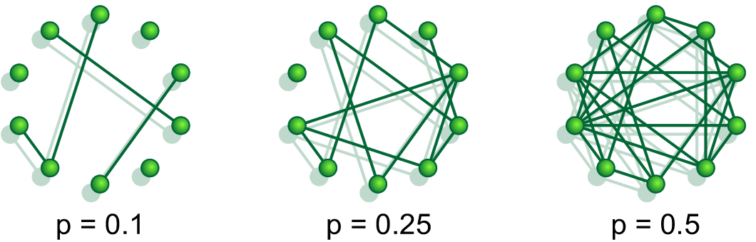
Figure 1: Evolution process of a classical random graph with $N=10$ nodes: starting from isolated nodes, we randomly add edges with increasing probability $p$, to eventually get the complete graph $K_{10}$ for $p=1$.

A classical network is mathematically represented by a graph, which is a pair of sets $G=(V,E)$ where $V$ is a set of $N$ nodes (or vertices) and $E$ is a set of $L$ edges (or links) connecting two nodes. The theory of random graphs, aiming to tackle networks with a complex topology, considers graphs in which each pair of nodes $i$ and $j$ are joined by a link with probability $p_{i,j}$. The simplest and most studied model is the one where this probability is independent of the nodes, with $p_{i,j}=p$, and the resulting graph is denoted $G_{N,p}$. The construction of these graphs can be considered as an evolution process: starting from $N$ isolated nodes, random edges are successively added and the obtained graphs correspond to larger and larger connection probability, see Fig. 1. One of the main goals of random-graph theory is to determine at which probability $p$ a specific property $P$ of a graph $G_{N,p}$ mostly arises, as $N$ tends to infinity. Many properties of interest appear suddenly, i.e. there exists a critical probability $p_{c}(N)$ such that almost every graph has the property $P$ if $p\geq p_{c}(N)$ and fails to have it otherwise; such a graph is said to by typical. For instance, the critical probability for the appearance of a given subgraph $F$ of $n$ nodes and $l$ edges in a typical random graph is Bollobás (1985):

$$p_{c}(N)=c\,N^{-n/l},$$ (1)

with $c$ independent of $N$. It is instructive to look at the appearance of subgraphs assuming that $p(N)$ scales as $N^{z}$, with $z\in(-\infty,0]$ a tunable parameter: as $z$ increases, more and more complex subgraphs emerge, see Tab. 1.

$\,z\,\vphantom{\frac{|^{|}}{|_{|}}}$	$-\infty$	$-2$	$-\frac{3}{2}$	$-\frac{4}{3}$	$-1$	$-\frac{2}{3}$

Table 1: Some critical probabilities at which a given subgraph $F$ appears in classical random graphs of $N$ nodes connected with probability $p\sim N^{z}$: cycles and trees of all orders appear at $z=-1$, while complete subgraphs (of order four or more) appear at a higher connection probability Albert and Barabási (2002).

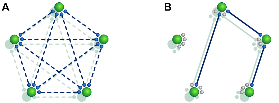
Figure 2: An example of a quantum random graph on five nodes. (A) Each node is in possession of four qubits which are entangled with qubits belonging to the other nodes. All the connections are identical and pure but non-maximally entangled pairs. (B) Imperfect pairs can be converted into maximally entangled ones with some probability of success $p$ (here $p=0.25$); this strategy mimics the behavior of classical random graphs.

We consider now the natural extension of the previous scenario to a quantum context. For each pair of nodes we replace the probability $p_{i,j}$ by a quantum state $\rho_{i,j}$ of two qubits, one at each node. Hence every node possesses $N-1$ qubits which are pairwise entangled with the qubits of the other nodes, as depicted in Fig. 2. The goal is then to establish maximally entangled states within certain subsets of nodes by using protocols that consist of local operations and classical communication (LOCC) Werner (1989), where each node can apply different measurements on its quantum system and then communicates its results to the rest. This is in fact a very natural scenario since maximally entangled states are the resource for most quantum information tasks, and thus the goal of any strategy. As in the classical random graphs we consider that pairs of qubits are identically connected, with $\rho_{i,j}=\rho$. Furthermore, we restrict ourselves to the simplest case where the states are pure, i.e. $\rho=\,|\varphi\rangle\negthinspace\langle\varphi|\,$, since it already leads to some very intriguing phenomena. We take these states to be:

$$\,|\varphi\rangle=\sqrt{1-p/2}\,|00\rangle+\sqrt{p/2}\,|11\rangle,$$ (2)

where $0\leq p\leq 1$ measures the degree of entanglement of the links. As before $p$ scales with $N$ and we write $\,|G_{N,p}\rangle$ the corresponding quantum random graph. The choice of the coefficients in Eq. (2) becomes clear if one considers the following simple strategy where links are treated independently: each pair of qubits tries to convert its connection by LOCC into the maximally entangled state $\,|\Phi^{+}\rangle\propto\,|00\rangle+\,|11\rangle$. The probability of a successful conversion is $p$, which is optimal Nielsen (1999); Vidal (1999), and therefore the task of determining the type of maximally entangled states remaining after these conversions can be exactly mapped to the classical problem. In that case we obtain the results of Tab. 1, and for example for $z\geq-2$ the probability to find a pair of nodes that share a maximally entangled state is one, whereas that of having three nodes sharing three maximally entangled states is zero unless $z\geq-1$.

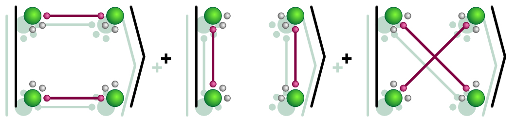
Figure 3: Graphical representation of $\,|K_{c}\rangle$. Each node has exactly $c-1$ orthogonal states in which $c-2$ qubits are $\,|0\rangle$ and one is $\,|1\rangle$; qubits that were originally entangled share the same state. A link denotes, here, the separable state $\,|11\rangle$ while $\,|00\rangle$ is not drawn, and $\,|K_{c}\rangle$ is defined as the coherent superposition of all perfect matchings of the complete graph $K_{c}$. In this example an appropriate labeling of the states leads to $\,|K_{4}\rangle\propto\,|1111\rangle+\,|2222\rangle+\,|3333\rangle$.

Allowing strategies which entangle the qubits within the nodes offers new possibilities and brings powerful results. This is indeed a general fact in quantum information theory as, for example, in the context of distillation of entanglement Bennett et al. (1996) or in the non-additivity of the classical and quantum capacity of quantum channels Hastings (2009). As a first illustration of the advantage of joint actions on qubits we show how some relevant multipartite entangled states, like the three-dimensional Greenberger-Horne-Zeilinger (GHZ) Greenberger et al. (1989) state of four particles, can be obtained when $z=-2$. At each node we apply a generalized (or incomplete) measurement Nielsen and Chuang (2000) whose elements $P_{m}$ are projectors onto the subspaces consisting of exactly $m$ qubits in the state $\,|1\rangle$, i.e. we count the number $m$ of “links” $\,|11\rangle$ attached to the nodes without revealing their precise location. Remark that such links are separable and so do not represent the sought connections $\,|\Phi^{+}\rangle$. For each measurement we get a random outcome $m$ whose value is either $0$ or $1$ since, as in the classical case, the probability to get $m\geq 2$ is zero for infinite $N$ Bollobás (1981), see App. A. Setting $p=2cN^{-2}$ one finds that there are in average $c$ nodes having exactly one qubit in the state $\,|1\rangle$, whereas all nodes where $m=0$ factor out since they are completely uncorrelated with the rest of the system. In Fig. 3 we describe the remaining state, which we write $\,|K_{c}\rangle$, and show that for $c=4$ it is a GHZ state of four qutrits.

We now turn to the main result of this paper: for $N$ tending to infinity and with $p\sim N^{-2}$ one is able to obtain with unit probability a quantum state with the structure of any finite subgraph. That is, for an arbitrary subgraph $F=(V,E)$ composed of $n$ vertices and $l$ edges, one can get the state $\,|F\rangle$ consisting of $l$ maximally entangled pairs $\,|\Phi^{+}\rangle$ shared among $n$ nodes, according to $E$:

$$\,|F\rangle=\bigotimes_{i=1}^{l}\,|\Phi^{+}\rangle_{E_{i}}.$$ (3)

This result implies that in the quantum case the structure of Tab. 1 completely changes, as all subgraphs already appear at $z=-2$. Actually, our results are more general since any state of some interest in quantum information theory, as W states, Dicke states, graph states, etc., also arise at $z=-2$. We sketch here the four steps of our proof and refer the reader to App. B for detailed calculations. First, we create the state $\,|K_{c}\rangle$ described in Fig. 3, with $c=n+D$, $D=d^{2}$ and $d=2^{l}$: $n$ nodes will be kept to build the final state while $D$ additional nodes are needed to establish the desired quantum correlations. Second, we measure all links corresponding to the subgraph $K_{n}$ and the other $D$ vertices are measured in the Fourier basis, which leads to a highly entangled state of $n$ nodes of dimension $D$. Third, in order to extract the right correlations, we split each node into two subsystems of dimension $d$, measure one of them in the Fourier basis and post-select a specific outcome pattern. Finally, we show that the resulting state, a $n$-partite GHZ state of dimension $d$, can be converted into $\,|F\rangle$ by some appropriate projections.

At this point let us briefly describe a possible setup for an implementation of our ideas, where atoms store the quantum information, and thus represent qubits, while photons are used to create remote entanglement. This scenario is currently well admitted to be the most promising one for a realization of quantum networks Kimble (2008). In particular, we consider the case where (continuous-variable) entanglement contained in a two-mode squeezed light is transformed into (discrete) entanglement between atoms trapped in distant high-quality cavities Kraus and Cirac (2004). Assuming perfect operations one can drive the system so that its steady state is exactly described by Eq. 2, with $p<1$ due to a finite squeezing of the light. In App. C we discuss a simple model of mixed-state networks where the source of squeezed states fails to emit, with some probability, any light. We show that the quantum phenomena considered so far persist despite these imperfections, and we believe that this will still be the case for more general types of errors.

In conclusion, we have introduced a model of complex quantum networks based on the theory of random graphs and have shown that allowing joint actions on the nodes dramatically changes one of their main properties, namely the appearance of subgraphs according to the connection probability. In fact, all classical exponents collapse onto the value $z=-2$ in the quantum case and we expect a large variety of new phenomena in, for instance, quantum models of small-world or scale-free networks. The model we have introduced is quite simple in the sense that connections are represented by pure states, whereas more realistic setups involve mixed states. We discussed this problem for a specific type of imperfections, and even if it may be much more difficult to tackle it in full generality we are confident of the persistence of unexpected and intriguing phenomena in real quantum networks. We hope that our results will inspire work in this direction and shed some light on the very active domain of complex networks.

Appendix A: General considerations and notation

As in the classical case we consider the exponent $z$ in $p=N^{z}$ to be larger than or equal to $-2$, since the overlap of the quantum random graph and the product state $\,|\vec{0}\rangle$ of all qubits in $\,|0\rangle$ approaches unity for $z<-2$ and in the limit of infinite lattices:

$$|\langle G_{N,p}|\vec{0}\rangle|^{2}=\left(1-\frac{p}{2}\right)^{\frac{N(N-1)}{2}}\simeq\exp\Big{(}\frac{-N^{z+2}}{4}\Big{)}\rightarrow 1,$$

and therefore no local quantum operation is able to create entanglement between nodes in this case. Furthermore, the outcome distribution of the measurements $P_{m}$ follows the classical degree distribution of a random graph $G_{N,p^{\prime}}$, with $p^{\prime}=p/2$. In fact the only information we get from $\,|G_{N,p}\rangle$ by applying $P_{m}$ is the number of links $\,|11\rangle$ attached to a given node, and each such link gets a weight $p/2$ in the outcome probabilities. This distribution has been shown to be well approximated by the one that we get if the nodes are considered to be independent, so that the expected number $x_{m}$ of outcomes $m$ reads, setting $p=2cN^{z}$ and for $z<-1$:

$$E(x_{m}) =\frac{N!}{m!\,(N-1-m)!}\left(\frac{p}{2}\right)^{m}\left(1-\frac{p}{2}\right)^{N-1-m}$$

$$\simeq\frac{c^{m}}{m!}N^{m(z+1)+1}.$$ (4)

In the text we often mention the act of measuring a node, or more generally of a system of dimension $d$: if no basis is specified we mean a measurement in the computational basis, i.e. we project the system onto the states $\,|1\rangle,\ldots,\,|d\rangle$. We also use the expression “to measure a link” to indicate that one of its qubits is measured in the $\{\,|0\rangle,\,|1\rangle\}$ basis. Finally, we introduce the notation

$$\,|\Phi_{n}^{k,d}\rangle=\frac{1}{\sqrt{d}}\sum_{j=1}^{d}e^{\frac{2\pi i}{d}jk}\,|\underbrace{jj\ldots j}_{n}\rangle,\quad k\in\{1,\ldots,d\},$$ (5)

for the Fourier transform of $\,|\Phi_{n}^{d}\rangle\equiv\,|\Phi_{n}^{d,d}\rangle$. The latter state is referred in the text as a GHZ state of dimension $d$ (on $n$ nodes), and a measurement in the Fourier basis of a system of dimension $d$ is its projection onto the states $\,|\Phi_{1}^{k,d}\rangle$.

Appendix B: Proof of the main result

We give here the details of the construction of a state $\,|F\rangle$, starting from $\,|G_{N,p}\rangle$ and using LOCC only. But let us first note that if one is able to find a construction which succeeds with a strictly positive probability, say $p_{F}$, that does not depend on $N$ but on the subgraph $F$ only, then $\,|F\rangle$ can be obtained with a probability arbitrary close to one. The reason is that we can always subdivide the $N$ nodes into $L$ sets of $N/L$ nodes, with $L\gg 1/p_{F}$, and apply the same construction on each set. These sets can be treated as independent if we initially discard all links connecting different sets, which is done by measuring the corresponding qubits. Note that in what follows we do not try to optimize the procedure since in the limit of infinite $N$ we are mainly interested in the existence of a finite probability $p_{F}$, not in its maximal possible value.

First step. We start the construction by creating the state $\,|K_{c}\rangle$, with $c=n+D$, $D=d^{2}$ and $d=2^{l}$, which can be obtained with a probability approaching unity in the limit of infinite $N$. In fact one can choose a value $c^{\prime}\gg c$, apply the projections $P_{m}$ on the nodes of the quantum network and get a system of average size $c^{\prime}$. The number of nodes of the resulting state can then be decreased in a deterministic fashion: one measures all qubits of a node, gets $0$ for all outcomes except for a random one whose neighbor automatically factors out. Hence, the system is projected onto $\,|K_{c^{\prime}-2}\rangle$ and the procedure can be iterated until we get $\,|K_{c}\rangle$.

Second step. We remove all connections shared between $n$ nodes of $\,|K_{c}\rangle$, i.e. we measure the $n(n-1)/2$ concerned links, and the operation is successful if all outcomes are 0. In that way we build a state that is the coherent superposition, as described in Fig. 3, of all perfect matchings of the join graph of $K_{D}$ and of the empty graph on $n$ nodes. We further measure these $D$ nodes, but this time in the Fourier basis $\{\,|\Phi_{1}^{k,c-1}\rangle,1\leq k\leq c-1\}$ in order not to reveal where the links $\,|11\rangle$ lie. We can correct the possibly introduced phases and the resulting state reads:

$$\,|\varphi_{n}^{D}\rangle\propto\sum_{i_{1}\neq i_{2}\ldots\neq i_{n}=1}^{D}\,|i_{1}i_{2}\ldots i_{n}\rangle.$$ (6)

Third step. It is not convenient to deal with sums whose indices are subject to constraints, so we develop Eq. 6 to let the sums freely run from $1$ to $D$. For example, the state on three nodes is expressed as:

$$\,|\varphi_{3}^{D}\rangle=\sum_{i,j,k=1}^{D}\,|ijk\rangle-\sum_{i,j=1}^{D}\big{(}\,|iij\rangle+\,|iji\rangle+\,|jii\rangle\big{)}+2\sum_{i=1}^{D}\,|iii\rangle.$$

More generally this leads to a weighted and symmetric superposition of states of the form $\bigotimes_{i=1}^{r}\,|\Phi_{\lambda_{i}}^{D}\rangle$ for all partitions $(\lambda_{1},\lambda_{2},\ldots,\lambda_{r})$ of $n$, where $\sum_{i=1}^{r}\lambda_{i}=n$ (a partition of a positive integer is a way of writing it as a sum of positive integers). We want to remove all terms of this sum but the last one, which is a GHZ state that will allow us to obtain $\,|F\rangle$. To that purpose we use the fact that $\,|\Phi_{n}^{D}\rangle=\,|\Phi_{n}^{d^{2}}\rangle=\,|\Phi_{n}^{d}\rangle^{\otimes 2}$ for all $n$ and $d$, split each node into two subsystems of dimension $d$ and measure one of them in the Fourier basis. This operation is successful if all outcomes are $k=1$, except the last one which should be $k=d-n+1$. In fact, to see what happens to a state $\,|\Phi_{m}^{d}\rangle$ we note that $\langle\Phi_{1}^{k,d}|\Phi_{m}^{j,d}\rangle\propto\,|\Phi_{m-1}^{j-k,d}\rangle$ if $m>1$ and $\delta_{j,k}$ otherwise. Therefore, by sequentially measuring $\langle\Phi_{1}^{1,d}|\,$, a state $\,|\Phi_{m}^{d}\rangle$ shared among any $m<n$ nodes transforms as:

$$\,|\Phi_{m}^{d}\rangle\equiv\,|\Phi_{m}^{d,d}\rangle\mapsto\,|\Phi_{m-1}^{d-1,d}\rangle\mapsto\ldots\mapsto\,|\Phi_{1}^{d-m+1,d}\rangle\mapsto 0,$$

as long as $d>m$. But this is always the case because, without loss of generality, the subgraph can be considered to be connected, so that $l\geq n-1$ and thus $d\geq 2^{l}\geq 2^{n-1}\geq n>m$. Hence all terms vanish except the GHZ state $\,|\Phi_{n}^{d}\rangle$.

Fourth step. The last step consists in transforming $\,|\Phi_{n}^{d}\rangle$ into $\,|F\rangle$. To that end first expand Eq. 3, i.e. write explicitly all its terms in the computational basis, and group the qubits according to the connections $E$. This leads to a sum of product states of the form $\,|\varphi_{i,1}\rangle\ldots\,|\varphi_{i,n}\rangle$ with $i=1,\ldots,2^{l}$. Since we have chosen $d=2^{l}$, we can now apply the measurement element $\sum_{i=1}^{d}\,|\varphi_{i,j}\rangle\negthinspace\langle i|\,$ on each node $j$ of $\,|\Phi_{n}^{d}\rangle$, which achieves the desired transformation and concludes the proof.

Appendix C: A mixed-state scenario

Figure 4: Scheme for entanglement generation between two nodes: two distant cavities are simultaneously driven by a common source $S$ of squeezed light, and in the steady state of the system the two atoms $A$ and $B$ become entangled.

We consider here the setup described in Kraus and Cirac (2004), where two high-quality cavities are simultaneously driven by a common source of two-mode squeezed light, see Fig. 4. The continuous-variable entanglement contained in the light is transformed into discrete entanglement between atoms, and the steady state of the system is described by the non-maximally entangled pure state we use throughout the text. Let us now introduce some errors into the networks, considering an imperfect source of light which fails to emit squeezed states with some probability $\varepsilon$. Equivalently, this imperfect source produces the vacuum state $\,|00\rangle$ with probability $\varepsilon$ so that the connections of the quantum network are:

$$\rho=(1-\varepsilon)\,|\varphi\rangle\negthinspace\langle\varphi|\,+\varepsilon\,|00\rangle\negthinspace\langle 00|\,,$$ (7)

with $\,|\varphi\rangle$ defined in Eq. 2. For this error we can show that it is still possible to construct, in the regime $z=-2$, mixed states which are close to arbitrary quantum subgraphs. To that end let us go through the four steps of the construction described in the previous paragraph. The first step consists in creating the state $\,|K_{c}\rangle$ by applying the measurements $P_{m}$ on the nodes of the network. These measurements are not affected by the imperfect source since no extra links $\,|11\rangle$ are added: only the number of outcomes $m=1$ slightly decreases from $c$ to $(1-\varepsilon)c$, but one can choose a larger constant $c^{\prime}$ in $p=2c^{\prime}N^{-2}$ in order to get with certainty $c$ outcomes $P_{1}$. For $c=4$ for instance, the remaining nodes are in a mixture of the desired state $\,|K_{4}\rangle$ and some completely separable states:

$$\rho_{K4}=x\,|K_{4}\rangle\negthinspace\langle K_{4}|\,+\frac{1-x}{3}\sum_{i=1}^{3}\,|iiii\rangle\negthinspace\langle iiii|\,,$$ (8)

with $x=(1-\varepsilon)^{2}$ for infinite $N$. Despite the presence of separable states, $\rho_{K4}$ is useful for quantum information tasks since it is distillable for all $\varepsilon<1$, i.e. the coefficient $x$ can be brought arbitrarily close to unity if one possesses a large number of copies of it. However, in the regime $z=-2$ it is impossible to get several copies of $\rho_{K4}$ on the same four nodes. But this is not a problem since, alternatively, we can repeat the construction $1/x$ times so that any use of $\,|K_{c}\rangle$ is still achieved with high probability. More generally, the state $\rho_{Kc}$ on $c$ nodes is a mixture of $\,|K_{c}\rangle$ and of some partially separable states, with $x$ equal to $(1-\varepsilon)^{c/2}$. Note that all terms appearing in $\rho_{Kc}$ are also present in $\,|K_{c}\rangle$, but they now are probabilistically weighted. This structure is maintained throughout the construction of the quantum subgraphs (steps two to four of the proof), so that with probability $x$ we create $\,|F\rangle$, and with probability $1-x$ we get a sum of useless quantum states. Therefore, for all $\varepsilon<1$, with a strictly positive probability we can achieve quantum communication or computation that is impossible within a classical framework.

In conclusion, we have discussed a possible implementation of our model of quantum networks and shown that the proposed construction of quantum subgraphs is robust against some specific imperfections, namely a noise $\,|00\rangle\negthinspace\langle 00|\,$ from the light sources. Remark that this is not the case for errors involving terms like $\,|01\rangle\negthinspace\langle 01|\,$, $\,|10\rangle\negthinspace\langle 10|\,$ or $\,|11\rangle\negthinspace\langle 11|\,$ in the connections. However, in that case, we are confident that other quantum strategies (based on purification methods for instance) will still lead to intriguing and powerful phenomena, thus stimulating further work on complex quantum networks.

References

- Albert and Barabási (2002) R. Albert and A.-L. Barabási, Rev. Mod. Phys. 74, 47 (2002).
- Erdős and Rényi (1959) P. Erdős and A. Rényi, Publ. Math. Debrecen 6, 290 (1959).
- Erdős and Rényi (1960) P. Erdős and A. Rényi, Publ. Math. Inst. Hung. Acad. Sci. 5, 17 (1960).
- Erdős and Rényi (1961) P. Erdős and A. Rényi, Bull. Inst. Int. Stat. 38, 343 (1961).
- Watts and Strogatz (1998) D. J. Watts and S. H. Strogatz, Nature 393, 440 (1998).
- Barabási and Albert (1999) A.-L. Barabási and R. Albert, Science 286, 509 (1999).
- Kimble (2008) H. J. Kimble, Nature 453, 1023 (2008).
- Gisin and Thew (2007) N. Gisin and R. Thew, Nature Photon. 1, 165 (2007).
- Acín et al. (2007) A. Acín, J. I. Cirac, and M. Lewenstein, Nature Phys. 3, 256 (2007).
- Perseguers et al. (2008) S. Perseguers, J. I. Cirac, A. Acín, M. Lewenstein, and J. Wehr, Phys. Rev. A 77, 022308 (2008).
- Bollobás (1985) B. Bollobás, Random graphs (Academic Press, London, 1985).
- Werner (1989) R. F. Werner, Phys. Rev. A 40, 4277 (1989).
- Nielsen (1999) M. A. Nielsen, Phys. Rev. Lett. 83, 436 (1999).
- Vidal (1999) G. Vidal, Phys. Rev. Lett. 83, 1046 (1999).
- Bennett et al. (1996) C. H. Bennett, G. Brassard, S. Popescu, B. Schumacher, J. A. Smolin, and W. K. Wootters, Phys. Rev. Lett. 76, 722 (1996).
- Hastings (2009) M. B. Hastings, Nature Phys. 5, 255 (2009).
- Greenberger et al. (1989) D. M. Greenberger, M. A. Horne, and A. Zeilinger, Bell’s theorem, Quantum Theory, and Conceptions of the Universe (Kluwer Academics, Dordrecht, 1989).
- Nielsen and Chuang (2000) M. A. Nielsen and I. L. Chuang, Quantum Computation and Quantum Information (Cambridge University Press, 2000).
- Bollobás (1981) B. Bollobás, Discrete Math. 33, 1 (1981).
- Kraus and Cirac (2004) B. Kraus and J. I. Cirac, Phys. Rev. Lett. 92, 013602 (2004).