Least zero of a cubic form

Abstract

An effective search bound is established for the least non-trivial integer zero of an arbitrary cubic form $C\in\mathbb{Z}[X_{1},\ldots,X_{n}]$, provided that $n\geqslant 17$.

1. Introduction

Let $n\geqslant 3$ and let $F\in\mathbb{Z}[X_{1},\ldots,X_{n}]$ be an indefinite form of degree $d\geqslant 2$, with coefficients of maximum modulus $\|F\|$ and greatest common divisor $1$. It is very natural to try and ascertain procedures for determining whether or not the equation $F=0$ is soluble in integers. One such approach involves providing an effective upper bound for the smallest positive integer $\lambda$ with the property that when there is a non-zero solution $\mathbf{x}=(x_{1},\ldots,x_{n})\in\mathbb{Z}^{n}$ to the equation $F=0$, so there is such a solution with $\max_{1\leqslant i\leqslant n}|x_{i}|\leqslant\lambda$. Let us denote this quantity by $\Lambda_{n}(F)$ when it exists.

When $d=1$ the problem is straightforward, and it follows from Siegel’s lemma that $\Lambda_{n}(F)\leqslant n^{\frac{1}{n-1}}\|F\|^{\frac{1}{n-1}}$. For polynomials of higher degree the problem has received the most attention in the case $d=2$ of quadratic forms $F=Q$. There is a well-known result due to Cassels [4], which shows that

$$\Lambda_{n}(Q)\leqslant c_{n}\|Q\|^{\frac{n-1}{2}},$$

with a completely explicit value of $c_{n}$. Although the exponent of $\|Q\|$ is known to be best possible in general, recent joint work of Browning and Dietmann [3] demonstrates that one can do much better for generic quadratic forms. It is interesting to remark that Cassels’ bound played an important rôle in the work of Birch and Davenport [2] on the solubility in integers of Diophantine inequalities $|Q(x_{1},\ldots,x_{n})|<1,$ for suitable quadratic forms $Q$ defined over $\mathbb{R}$.

The situation for forms of degree $d=3$ is far less satisfactory, and a proper analogue of Cassels’ result for quadratic forms remains a distant prospect. Aside from the intrinsic interest of this problem, such a bound would be very desirable in the context of cubic Diophantine inequalities.

Let us record some of the progress that has been made for cubic forms $F=C$. Suppose first that the form is diagonal and has $7$ variables, with coefficients $A_{1},\ldots,A_{7}$. Then Li [14] has shown that there is a non-trivial integral solution with

$$\sum_{i=1}^{7}|A_{i}x_{i}^{3}|\leqslant c|A_{1}\cdots A_{7}|^{14},$$

for some absolute constant $c>0$. In particular it easily follows from this result that $\Lambda_{n}(C)\leqslant c\|C\|^{\frac{95}{3}},$ for any diagonal cubic form in $n\geqslant 7$ variables.

For general cubic forms one of the few results in the literature is due to Pitman [16]. For any $\varepsilon>0$, Pitman establishes the existence of constants $N_{\varepsilon}$ and $c_{n,\varepsilon}>0$ such that

$$\Lambda_{n}(C)\leqslant c_{n,\varepsilon}\|C\|^{\frac{25}{6}+\varepsilon},$$

whenever $n\geqslant N_{\varepsilon}$. One notes that the exponent of $\|C\|$ is independent of $n$, unlike the situation for quadratic forms discussed above. However, the number of variables needed to make this argument work is extremely large. This loss is due to the wasteful nature of the proof, in which a diagonalisation process is applied to reduce the problem to bounding $\Lambda_{n}(C)$ for a diagonal cubic form. Still working with cubic forms in many variables, it has been shown by Schmidt [17, Theorem 2] that Pitman’s estimate is valid with the exponent $\frac{25}{6}$ replaced by a function $e_{1}(n)$ that tends to $0$ as $n\rightarrow\infty$.

At the expense of a much weaker exponent of $\|C\|$, it is nonetheless possible to produce estimates for $\Lambda_{n}(C)$ when $n$ is as small as $17$, by avoiding the use of diagonalisation arguments. This is the point of view adopted by Elliott [8] in his Ph.D. thesis, where it is shown that there exists a constant $c_{n}>0$ such that

$$\Lambda_{n}(C)\leqslant c_{n}\|C\|^{e_{2}(n)},$$

for $n\geqslant 17$, where

$$e_{2}(n)=\begin{cases}\{1+\frac{3}{4}(\frac{n+24}{n-16})(\frac{11n(n-1)}{n-9}+10n-13)\}\{\frac{(2n+3)^{2}}{8}-n-1\},&\mbox{if $n\leqslant 30$,}\\ n\{1+\frac{3}{4}(\frac{3n+120}{3n-80})(\frac{11n(n-1)}{n-9}+10n-13)\},&\mbox{if $n\geqslant 30$.}\end{cases}$$

Taking $n=17$ one finds that $e_{2}(17)=2500417$. In later work, seemingly unaware of Elliott’s thesis, Lloyd [15] succeeded in showing that

$$\Lambda_{17}(C)\leqslant c\|C\|^{8\times 10^{8}},$$

for some absolute constant $c>0$ and any non-singular cubic form in $17$ variables. Thus Lloyd’s exponent is worse than that obtained by Elliott and has the defect of only applying to non-singular cubic forms.

The primary aim of this paper is to stimulate further interest in this and allied problems. Our main achievement will be a sharper upper bound for $\Lambda_{n}(C)$ when $n\geqslant 17$. The following result deals with cubic forms $C$ for which the corresponding hypersurface $C=0$ has a suitably restricted singular locus.

Theorem 1.

Let $C\in\mathbb{Z}[X_{1},\ldots,X_{n}]$ be a cubic form, with $n\geqslant 17$, defining a hypersurface with at most isolated ordinary singularities. Then for any $\varepsilon>0$ there exists a constant $c_{n,\varepsilon}>0$ such that

$$\Lambda_{n}(C)\leqslant c_{n,\varepsilon}\|C\|^{e_{3}(n)+\varepsilon},$$

where

$$e_{3}(n)=\begin{cases}\frac{22n^{3}+107n^{2}-597n-432}{(n-2)(n-16)(n-9)},&\mbox{if $n\leqslant 20$,}\\ \frac{n^{4}+125n^{3}+1518n^{2}-7236n-4320}{32(n-2)(n-9)},&\mbox{if $n>20$.}\end{cases}$$ (1.1)

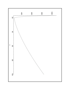
Figure 1. The function $e_{3}(n)$ for $17\leqslant n\leqslant 100$

The constant $c_{n,\varepsilon}$ in Theorem 1 is effectively computable, a feature shared by all the implied constants in this work. In Figure 1 we have graphed the function $e_{3}(n)$ for small values of $n$. Taking $n=17$ and $\varepsilon$ sufficiently small, one concludes from Theorem 1 that

$$\Lambda_{17}(C)\leqslant c\|C\|^{1071}$$

for an absolute constant $c>0$, provided that the hypersurface $C=0$ is non-singular or contains isolated ordinary singularities. When $n=20$ this exponent can be improved to $261$. Theorem 1 provides a palpable improvement over the earlier works of Elliott or Lloyd discussed above. In fact $e_{3}(n)\sim\frac{1}{32}n^{2}$, as $n\rightarrow\infty$, whereas $e_{2}(n)\sim\frac{63}{4}n^{2}$.

It is natural to ask what can be said about arbitrary cubic forms. At the expense of a weaker exponent, we answer this in the following result.

Theorem 2.

Let $C\in\mathbb{Z}[X_{1},\ldots,X_{n}]$ be a cubic form, with $n\geqslant 17$. Then there exists an absolute constant $c>0$ such that

$$\Lambda_{n}(C)\leqslant c\|C\|^{360000}.$$

All of the bounds for $\Lambda_{n}(C)$ that we have discussed so far are based on applications of the Hardy–Littlewood circle method, and our approach is no exception. The informed reader will notice that the restriction to cubic forms in at least $17$ variables is at odds with current understanding of rational points on cubic hypersurfaces. Indeed, by employing the machinery of Hooley [11] one ought to be able to handle cubic forms that define hypersurfaces with at most isolated ordinary singularities in only $10$ variables. Similarly, for general cubic forms, the work of Heath-Brown [10] should allow a reduction from $n\geqslant 17$ to $n\geqslant 14$ in Theorem 2. Both of these improvements would be at the expense of considerable extra labour, however. In the present investigation we have decided to place the emphasis on brevity of exposition, and it is hoped that the deficiency alluded to above will be taken in the light of this fact.

The relative strength of our results arises from a more sophisticated treatment of the major arcs and of the positivity of the singular series. The latter phase of the argument hinges upon good lower bounds for the quantity

$$\varrho(p^{k})=\#\{\mathbf{x}\in(\mathbb{Z}/p^{k}\mathbb{Z})^{n}:C(\mathbf{x})\equiv 0\,(\operatorname{mod}{p^{k}})\},$$ (1.2)

for prime powers $p^{k}$. Taking $k=1$, the problem reduces to estimating the number of points on the cubic hypersurface $C=0$ over $\mathbb{F}_{p}$. We will seek estimates of the form $\varrho(p)=p^{n-1}+O(p^{n-\theta})$, where the implied constant depends at most on $n$. When $C$ is non-singular modulo $p$ the work of Deligne shows that $\theta=\frac{n}{2}$ is permissible. For general $C$ we can take $\theta=\frac{1}{2}$ by the Lang–Weil estimate, provided that $C$ is absolutely irreducible modulo $p$. This is not good enough for our purposes however. We circumvent this difficulty with the following result.

Theorem 3.

Let $C\in\mathbb{F}_{p}[X_{1},\ldots,X_{n}]$ for $n\geqslant 10$. Suppose further that $C$ is non-degenerate. Then

$$\varrho(p)\geqslant p^{n-1}+O(p^{n-2}),$$ (1.3)

where the implied constant depends at most on $n$.

The investigation of least non-trivial zeros of cubic forms is currently enjoying a resurgence of interest. The problem is most intriguing in the case $n=4$ of surfaces. As highlighted by Swinnerton-Dyer [19, Question 15], a real milestone in this domain would be to discover whether one could estimate $\Lambda_{4}(C)$ effectively when $C$ is diagonal. Elsenhans and Jahnel [9] have gone further, based on numerical calculations, asking whether one can expect inequalities of the sort

$$\Lambda_{4}(C)\leqslant\frac{c_{\varepsilon}}{\tau(C)^{1+\varepsilon}},$$

where $\tau(C)$ is a Tamagawa number associated to the corresponding cubic surface.

It would be interesting to explore whether the ideas in this paper could be adapted to handle non-singular forms of degree exceeding $3$. This would be in complete analogy to the extension by Birch [1] to higher degree of Davenport’s [5] treatment of cubic forms. It is easily checked that the treatment of minor and major arcs goes through with little alteration. The main obstacle appears to be achieving effective lower bounds for the singular integral and singular series, respectively.

Notation.

All of the implied constants in our work will be allowed to depend on $n$ and $\varepsilon$, with any further dependence being made completely explicit. We will adhere to common practice and allow $\varepsilon$ to take different values at different parts of the argument, but we shall always assume it to be very small. Throughout the remainder of the paper we write

$$M=\|C\|,$$

for the height of the cubic form $C$ that is under scrutiny, and $|\mathbf{x}|$ for the norm $\max_{1\leqslant i\leqslant n}|x_{i}|$ of any vector $\mathbf{x}\in\mathbb{R}^{n}$.

Acknowledgement.

While working on this paper the first author was supported by EPSRC grant number EP/E053262/1.

2. Skeletal proof of the theorems

We write our cubic form in the shape

$$C(x_{1},\ldots,x_{n})=\sum_{i,j,k}c_{ijk}x_{i}x_{j}x_{k},$$ (2.1)

in which the coefficients $c_{ijk}\in\mathbb{Z}$ are symmetric in the indices $i,j,k$. According to our hypothesis concerning notation the modulus of any coefficient $c_{ijk}$ is bounded by $M$. We claim that it will suffice to proceed under the assumption that $c_{111}$ is positive, with

$$c_{111}\gg M,$$ (2.2)

for an absolute implied constant.

Now it is already plain that there is no loss of generality in assuming that one of $|c_{111}|,|c_{112}|,|c_{123}|$ is at least $M$. Suppose that $|c_{123}|\geqslant M$ and for $\sigma\in\{-1,1\}$ consider the unimodular transformation

$$x_{i}\mapsto\begin{cases}y_{i},&\mbox{if $1\leqslant i\leqslant n$ and $i\neq 3$,}\\ \sigma y_{1}+y_{3},&\mbox{if $i=3$.}\end{cases}$$

This produces a new cubic form $C^{\prime}(y_{1},\ldots,y_{n})$ such that $\|C^{\prime}\|\ll M$, with integer coefficients $c_{ijk}^{\prime}(\sigma)$. In particular we have

$$|c_{112}^{\prime}(\sigma)|=|c_{112}+2\sigma c_{123}+c_{233}|=|2c_{123}|+|c_{112}+c_{233}|\geqslant 2M,$$

on choosing $\sigma$ to be the sign of $c_{123}^{-1}(c_{112}+c_{233})$.

Hence it suffices to assume that $|c_{112}|\geqslant M$ above. We now carry out the unimodular transformations

$$x_{i}\mapsto\begin{cases}y_{i},&\mbox{if $1\leqslant i\leqslant n$ and $i\neq 2$,}\\ \sigma y_{1}+y_{2},&\mbox{if $i=2$,}\end{cases}$$

for $\sigma\in\{-1,1\}$. If $|c_{111}^{\prime}(\sigma)|\geqslant\frac{M}{2}$ for either choice of $\sigma$ then we will be done. Alternatively, we have $\frac{M}{2}>|c_{111}^{\prime}(\sigma)|=|c_{111}+\sigma c_{112}+c_{122}+\sigma c_{222}|,$ for $\sigma=\in\{-1,1\}$. Choosing $\sigma$ to be the sign of $c_{111}+c_{122}$, we deduce that $|c_{112}+c_{222}|<\frac{M}{2}$, whence

$$|c_{222}|\geqslant|-c_{112}|-|c_{112}+c_{222}|\geqslant\frac{M}{2}.$$

On permuting the variables we can therefore assume that (2.2) holds in this case too. Note that the reduction from negative $c_{111}$ to positive $c_{111}$ is trivially achieved by multiplying the equation through by $-1$.

The basic idea behind the proof of Theorems 1 and 2 is very simple. Given a suitable bounded region $\mathscr{B}\subset\mathbb{R}^{n}$ we wish to establish an asymptotic formula for the counting function

$$N(P)=N_{\mathscr{B}}(P;C)=\sum_{\begin{subarray}{c}\mathbf{x}\in\mathbb{Z}^{n}\cap P\mathscr{B}\\ C(\mathbf{x})=0\end{subarray}}1,$$

as $P\rightarrow\infty$, uniformly in the coefficients of $C$. Here, $P\mathscr{B}=\{P\mathbf{x}:\mathbf{x}\in\mathscr{B}\}$. One then obtains explicit bounds on the size of $P$ needed to ensure that the main term dominates the error term in this estimate. For such $P$ we will thus have $N(P)>0,$ which then yields an upper bound for $\Lambda_{n}(C)$.

As indicated in the introduction we plan to use the Hardy–Littlewood circle method to estimate $N(P)$, based on the argument developed by Davenport [5]. For given $\mathbf{z}\in\mathbb{R}^{n}$ and $\varrho\in(0,1)$, let

$$\mathscr{B}=\mathscr{B}(\mathbf{z};\varrho)=\prod_{i=1}^{n}[z_{i}-\varrho,z_{i}+\varrho].$$

This is the box that we will work with. Note that $\operatorname{meas}(\mathscr{B})=2^{n}\varrho^{n}$. The choice of $\mathbf{z}$ and $\varrho$ will be made in due course, but we record now that

$$M^{-2-\frac{5}{n-2}}\ll\varrho\ll M^{-2-\frac{5}{n-2}},\quad|\mathbf{z}|\ll M^{\frac{1}{n-2}}.$$ (2.3)

Recall the definition (2.1) of the cubic form $C$. We define an $n\times n$ matrix $M(\mathbf{x})$ by taking its entries to be

$$M(\mathbf{x})_{jk}=\sum_{1\leqslant i\leqslant n}c_{ijk}x_{i}.$$ (2.4)

Let $\psi\in\mathbb{R}_{\geqslant 1}\cup\{\infty\}$. If one writes $r(\mathbf{x})=\operatorname{rank}(M(\mathbf{x}))$, then we shall say that $C$ is “$\psi$-good” if for any $\varepsilon>0$ the estimate

$$\#\{\mathbf{x}\in\mathbb{Z}^{n}:|\mathbf{x}|\leqslant H,\,r(\mathbf{x})=r\}\ll H^{r+\varepsilon}$$ (2.5)

holds for each $0\leqslant r\leqslant n$ and any $H$ in the range $1\leqslant H\leqslant M^{\psi}.$ Although we will not make this restriction yet, it turns out that our work is optimised by taking $\psi=\infty$ for the proof of Theorem 1 and $\psi=2646$ for the proof of Theorem 2.

An $\infty$-good form is one for which (2.5) holds for each $0\leqslant r\leqslant n$ and $H\geqslant 1$. It follows from work of Hooley [11, Lemma 28] that cubic forms defining a hypersurface with at most isolated ordinary singularities are all $\infty$-good. The following result, which will be proved in §3, handles the possibility that $C$ fails to be $\psi$-good, for a given choice of $\psi$.

Proposition 1.

Let $n\geqslant 3$ and let $\psi\geqslant 1$. Then either $C$ is $\psi$-good or

$$\Lambda_{n}(C)\ll M^{\frac{n^{2}}{2}-1+\frac{\psi n(n-1)}{2}}.$$ (2.6)

By our remarks above we may assume that the cubic forms considered in Theorem 1 are $\infty$-good. For a $\psi$-good cubic form $C$ we now desire an estimate for $N(P)$ in which the implied constant is completely uniform in $\varrho,\mathbf{z}$ and in the coefficients of $C$. Our starting point is the identity $N(P)=\int_{0}^{1}S(\alpha)\mathrm{d}\alpha,$ where

$$S(\alpha)=\sum_{\mathbf{x}\in\mathbb{Z}^{n}\cap P\mathscr{B}}e(\alpha C(\mathbf{x})).$$

We will always assume that $\varrho P\geqslant 1$, so that this sum is non-trivial. Let $P_{0}\geqslant 1$. We will take as major arcs

$$\mathfrak{M}(a,q)=\Big{[}\frac{a}{q}-\frac{P_{0}}{M\varrho^{3}P^{3}},\frac{a}{q}+\frac{P_{0}}{M\varrho^{3}P^{3}}\Big{]},$$

for given coprime integers $a,q$ such that $0\leqslant a<q\leqslant P_{0}$. The full set of major arcs is

$$\mathfrak{M}=\bigcup_{q\leqslant P_{0}}\bigcup_{\begin{subarray}{c}a=0\\ \mathrm{gcd}(a,q)=1\end{subarray}}^{q-1}\mathfrak{M}(a,q),$$

and the corresponding set of minor arcs is $\mathfrak{m}=[0,1]\setminus\mathfrak{M}$, defined modulo $1$. Our work will be optimised by taking

$$P_{0}=\big{(}M^{\frac{n}{8}}\varrho P\big{)}^{\frac{8}{n+16}}.$$ (2.7)

It is clear that $P_{0}\geqslant 1$. Note, furthermore, that the union of major arcs will be disjoint provided that $P_{0}\ll M^{\frac{1}{3}}\varrho P.$ Substituting in our choice of $P_{0}$, we see that this holds if and only if $\varrho P\gg M^{\frac{2(n-8)}{3(n+8)}}$, which follows from the assumption that

$$P\gg M^{15},$$ (2.8)

for $\varrho$ satisfying (2.3) and $n\geqslant 17$. Moreover, under this assumption it follows that

$$P_{0}\ll M^{\frac{n}{n+16}}P^{\frac{8}{n+16}}\ll M^{-4}P^{2}.$$ (2.9)

This will prove useful shortly.

The truncated singular series for our counting problem is given by

$$\SS(R)=\sum_{q\leqslant R}\sum_{\begin{subarray}{c}0\leqslant a<q\\ \mathrm{gcd}(a,q)=1\end{subarray}}q^{-n}\sum_{\mathbf{r}\,(\operatorname{mod}{q})}e_{q}(aC(\mathbf{r})),$$ (2.10)

for any $R\geqslant 1$. The assumption that our cubic forms are $\psi$-good is rather weak when $\psi<\infty$ and we cannot hope to establish the usual Hardy–Littlewood asymptotic formula for the full class of $\psi$-good cubic forms. In particular, the singular series $\SS=\lim_{R\rightarrow\infty}\SS(R)$ may fail to converge in general and we will be forced to work with the truncated series instead. The following two results handle the contribution from the minor arcs and major arcs, and will be established in §4 and §5, respectively.

Proposition 2.

Let $\varepsilon>0$ and assume that $n\geqslant 17$. Assume that $C$ is $\psi$-good and that $\varrho P\geqslant 1$. Then we have

$$\int_{\mathfrak{m}}|S(\alpha)|\mathrm{d}\alpha\ll M^{-\frac{\psi n}{4}}\varrho^{n}P^{n+\varepsilon}+M^{\frac{n}{8}-1}\varrho^{n-3}P^{n-3+\varepsilon}P_{0}^{2-\frac{n}{8}}.$$

Proposition 3.

Let $\varepsilon>0$ and assume that $n\geqslant 17$. Assume that $C$ is $\psi$-good and (2.8) holds. Then there exists a positive constant $\mathfrak{I}$ satisfying $\mathfrak{I}\gg\varrho^{n-1}M^{-1-\frac{2}{n-2}}$ such that

$$\int_{\mathfrak{M}}S(\alpha)\mathrm{d}\alpha=\SS(P_{0})\mathfrak{I}P^{n-3} +O\big{(}M^{-1}\varrho^{n-4}P^{n-4}P_{0}^{4}\big{)}$$

$$+O\big{(}M^{\frac{n}{8}+\frac{7}{2}+\frac{11}{n-2}}\varrho^{n-\frac{1}{2}}P^{n-3}P_{0}^{-\frac{1}{2}}\big{)}$$

$$+O\big{(}M^{6-\frac{\psi n}{4}}\varrho^{n}P^{n-3}P_{0}^{\frac{3}{2}+\varepsilon}\big{)}.$$

In our application we will take any $\varrho$ in the range (2.3), under which assumption we have

$$\mathfrak{I}\gg M^{-\frac{2n^{2}-1}{n-2}}$$ (2.11)

in Proposition 3. Furthermore, under (2.9), it follows that the third error term in this result is $O(M^{-\frac{\psi n}{4}}\varrho^{n}P^{n+\varepsilon}).$ Making the choice (2.7) for $P_{0}$, Propositions 2 and 3 combine to give the following result.

Proposition 4.

Let $\varepsilon>0$ and assume that $n\geqslant 17$. Assume that $C$ is $\psi$-good and (2.8) holds. Then we have

$$N(P)=\SS(P_{0})\mathfrak{I}P^{n-3} +O\big{(}M^{\frac{4n}{n+16}-1}(\varrho P)^{\frac{32}{n+16}+n-4+\varepsilon}\big{)}+O\big{(}M^{-\frac{\psi n}{4}}\varrho^{n}P^{n+\varepsilon}\big{)}$$

$$+O\big{(}M^{\frac{n(n+12)}{8(n+16)}+\frac{7}{2}+\frac{11}{n-2}}\varrho^{n-\frac{1}{2}-\frac{4}{n+16}}P^{n-3-\frac{4}{n+16}}\big{)}$$

$$+O\big{(}M^{\frac{n}{8}-1-\frac{n(n-16)}{8(n+16)}}\varrho^{n-3-\frac{n-16}{n+16}}P^{n-3-\frac{n-16}{n+16}+\varepsilon}\big{)}.$$

We have one major task remaining: we must establish an effective lower bound for the truncated singular series (2.10). This is probably the most challenging part of our argument. The following result will be proved in §7.

Proposition 5.

Let $\varepsilon>0$ and assume that $n\geqslant 17$. Suppose that (2.6) does not hold and that $C$ is $\psi$-good. If $\psi=\infty$ then

$$\SS(P_{0})\gg M^{-\frac{12n}{n-9}-\varepsilon}P_{0}^{-\varepsilon}-M^{\frac{n}{8}}P_{0}^{2-\frac{n}{8}+\varepsilon}.$$

If $\psi<\infty$ and $\delta$ satisfies

$$2<\delta<\frac{n}{8},\quad\frac{2n}{n-8\delta}<1+2\psi,$$ (2.12)

with $P_{0}\ll M^{1+2\psi}$, then we have

$$\SS(P_{0})\gg M^{-\frac{12n}{n-9}-\varepsilon}P_{0}^{-\varepsilon}-M^{\frac{n}{n-8\delta}+\varepsilon}P_{0}^{2-\delta+\varepsilon}.$$

We now have everything in place to deduce Theorems 1 and 2. Beginning with the former we suppose that $C$ defines a hypersurface with $n\geqslant 17$ variables and at most isolated ordinary singularities. Then we have already seen that $C$ is $\infty$-good by the work of Hooley [11, Lemma 28]. We will take

$$P=M^{e_{3}(n)+\varepsilon}$$

in Proposition 4, where $e_{3}(n)$ is given by (1.1). In particular it is clear that (2.8) holds for $n\geqslant 17$. With this choice of $P$, and for $\varrho$ in the range (2.3), we may combine the lower bound in (2.11) with the first part of Proposition 5 to conclude that

$$\SS(P_{0})\mathfrak{I}P^{n-3}\gg M^{(n-3)e_{3}(n)-\frac{2n^{2}-1}{n-2}-\frac{12n}{n-9}-\varepsilon}$$

in Proposition 4. We must now check that each error term in Proposition 4 is smaller than this bound with the above choice of $P$. This is clearly trivial for the second term, and for the the remaining terms it follows from a tedious calculation. Thus we may conclude that $N(P)>0$ for our choice of $P$, which therefore gives the statement of Theorem 1.

Turning to the deduction of Theorem 2, in which no restrictions are made upon the singular locus of $C=0$, we observe that for a given cubic form in $n>17$ variables we can always set $n-17$ of the variables equal to zero in order to obtain a cubic form in exactly $17$ variables. Thus it follows that we may proceed under the assumption that $n=17$. Following the argument above we will take

$$P=M^{E}$$

in Propositions 4 and 5 and we will optimise for $E$. In particular, taking $\varrho$ in the range (2.3), we see that (2.7) becomes

$$P_{0}=cM^{\frac{8E}{33}-\frac{5}{99}}.$$

for a suitable absolute constant $c>0$. We will assume that $E\geqslant 15$, so that (2.8) holds. Taking $n=17$ we note that if $C$ fails to be $\psi$-good, then Proposition 1 gives

$$\Lambda_{n}(C)\ll M^{143+\frac{1}{2}+136\psi},$$ (2.13)

with an absolute implied constant. We may suppose therefore that $C$ is $\psi$-good.

Under this assumption for $n=17$ we deduce that either (2.13) holds or else we can combine Propositions 4 and 5 with (2.11) to obtain

$$N(P)=\SS(P_{0})\mathfrak{I}P^{14} +O\big{(}M^{\frac{461E}{33}-\frac{3122}{99}+\varepsilon}+M^{17E-\frac{119}{3}-\frac{17\psi}{4}}\big{)},$$

for $E\geqslant 15$, with

$$\SS(P_{0})\mathfrak{I}P^{14}\gg M^{14E-\frac{577}{15}-\varepsilon}\big{(}M^{-\frac{51}{2}}-M^{\frac{17}{17-8\delta}+(2-\delta)({\frac{8E}{33}-\frac{5}{99}})}\big{)}.$$

The latter lower bound is for any $\delta$ such that (2.12) holds and is valid provided that $P_{0}\ll M^{1+2\psi}$, which forces upon us the additional constraint

$$\frac{8E}{33}-\frac{5}{99}\leqslant 1+2\psi.$$ (2.14)

Let us write $\delta=2+\delta_{0}$, say. Then the constraints in (2.12) become

$$0<\delta_{0}<\frac{1}{8},\quad\frac{34}{1-8\delta_{0}}<1+2\psi.$$ (2.15)

We observe that the first term dominates the second term in our lower bound for $\SS(P_{0})\mathfrak{I}P^{14}$ provided that

$$\frac{8E}{33}-\frac{5}{99}>\frac{1}{\delta_{0}}\Big{(}\frac{51}{2}+\frac{17}{1-8\delta_{0}}\Big{)}.$$

We will choose $\delta_{0}$ to minimise the right hand side, subject to the left hand condition in (2.15). Taking $\delta_{0}=0.076$ and selecting $E$ to be the least integer satisfying this inequality, we therefore deduce that $N(P)>0$ if

$$3739=E<\frac{17\psi}{12}-\frac{81}{10}.$$ (2.16)

Collecting together (2.14), (2.15) and (2.16), we conclude that $\Lambda_{n}(C)\ll M^{E}$ provided that $C$ is $\psi$-good for $\psi\geqslant 2646$. Note that the implied constant in this estimate is independent of $n$ since we are applying the circle method machinery at $n=17$. Taking $\psi=2646$ and combining this with (2.13), we therefore arrive at the statement of Theorem 2.

3. Elementary considerations

In this section we establish Proposition 1, thereby clearing the way for an application of the circle method. The following well-known result will prove useful, its proof being readily supplied by consulting [18, Lemma I.1], for example.

Lemma 1.

Let $m>k\geqslant 1$, and suppose that $\mathbf{a}_{1},\ldots,\mathbf{a}_{k}\in\mathbb{Z}^{m}$ are non-zero with modulus at most $A$. Then there exists $\mathbf{x}\in\mathbb{Z}^{m}$ such that

$$\mathbf{a}_{1}.\mathbf{x}=\cdots=\mathbf{a}_{k}.\mathbf{x}=0$$

and $0<|\mathbf{x}|\ll_{m}A^{\frac{k}{m-k}}$.

Our proof of Proposition 1 closely follows the argument of Davenport [5, §2], and so we will attempt to be brief. Let us write

$$B_{j}(\mathbf{x};\mathbf{y})=\sum_{i,k}c_{ijk}x_{i}y_{k},$$ (3.1)

for the $j$th bilinear form in the system $M(\mathbf{x})\mathbf{y}$. For given $\psi\geqslant 1$ we must deal with the possibility that $C$ fails to be $\psi$-good. Thus there exists $r\in\mathbb{Z}\cap[0,n]$ and $H\in\mathbb{Z}\cap[1,M^{\psi}]$ such that there are $\gg H^{n-r+\varepsilon}$ points $\mathbf{x}$, with $|\mathbf{x}|\leqslant H$, such that the bilinear equations $M(\mathbf{x})\mathbf{y}=\mathbf{0}$ have exactly $r$ linearly independent solutions in $\mathbf{y}$; that is, for which the matrix $M(\mathbf{x})$ has rank exactly $n-r$. In particular we may assume that $r\geqslant 1$, since there are $O(H^{n})$ integer vectors $\mathbf{x}$ with $|\mathbf{x}|\leqslant H$.

Our goal is to derive the existence of a solution $\mathbf{x}\in\mathbb{Z}^{n}$ to the equation $C(\mathbf{x})=0$, with

$$0<|\mathbf{x}|\ll M^{\frac{n^{2}}{2}-1}H^{\frac{n(n-1)}{2}}.$$ (3.2)

Given that $H\leqslant M^{\psi}$ this will therefore ensure that (2.6) holds, as required to conclude the proof of the proposition.

Let $\mathscr{X}$ denote the set of integer points $|\mathbf{x}|\leqslant H$ for which some particular minor of order $n-r$ is non-zero and all minors of order $n-r+1$ are zero. Then $\#\mathscr{X}\gg H^{n-r+\varepsilon}$, by assumption. For any $\mathbf{x}\in\mathscr{X}$, we suppose without loss of generality that the non-zero minor of order $n-r$, $\Delta$ say, lies in the top left-hand corner. It follows that solutions to the entire system of equations $M(\mathbf{x})\mathbf{y}=\mathbf{0}$ can be deduced from solutions to the first $n-r$ bilinear equations

$$B_{1}(\mathbf{x};\mathbf{y})=\cdots=B_{n-r}(\mathbf{x};\mathbf{y})=0.$$

For $1\leqslant i\leqslant r$, let $\Delta_{j}^{(i)}$ denote the determinant obtained from $\Delta$ by replacing the $j$th column by the $(n-r+i)$th column. Then an application of Cramer’s rule reveals that $r$ linearly independent solutions of the system $M(\mathbf{x})\mathbf{y}=\mathbf{0}$ are given by

$$\mathbf{y}^{(1)}= (\Delta_{1}^{(1)},\ldots,\Delta_{n-r}^{(1)},-\Delta,0,\ldots,0),$$

$$\vdots$$

$$\mathbf{y}^{(r)}= (\Delta_{1}^{(r)},\ldots,\Delta_{n-r}^{(r)},0,\ldots,0,-\Delta).$$

Note that each such vector is non-zero since $\Delta\neq 0$, and furthermore, has modulus $O((MH)^{n-r})$. Indeed, each $\Delta_{j}^{(i)},\Delta$ is a form in $\mathbf{x}$ of degree $n-r$ with integer coefficients of modulus $O(M^{n-r})$.

Now consider any point $\mathbf{Y}=\sum_{p=1}^{r}\lambda_{p}\mathbf{y}^{(p)}$ in the $r$-dimensional linear space spanned by $\mathbf{y}^{(1)},\ldots,\mathbf{y}^{(r)}$. Arguing as in the proof of [5, Lemma 3] we are led to the conclusion that

$$\sum_{j}\sum_{k}c_{\nu jk}Y_{j}Y_{k}+\sum_{k}\sum_{p=1}^{r}\lambda_{p}\Delta_{k}^{(p)}\frac{\partial Y_{k}}{\partial x_{\nu}}=\sum_{j}\sum_{p=1}^{r}\lambda_{p}Y_{j}\frac{\partial\Delta_{j}^{(p)}}{\partial x_{\nu}},$$ (3.3)

for each $1\leqslant\nu\leqslant n$. We now appeal to [5, Lemma 2], with $f_{1},\ldots,f_{N}$ being all the minors $\Delta_{j}^{(p)}$ of order $n-r+1$, for $1\leqslant j\leqslant n$ and $1\leqslant p\leqslant r$. Thus there is an element $\mathbf{x}\in\mathscr{X}$ for which all $\Delta_{j}^{(p)}$ are zero and for which the matrix

$$\Big{\{}\frac{\partial\Delta_{j}^{(p)}}{\partial x_{\nu}}\Big{\}}_{\begin{subarray}{c}1\leqslant j,\nu\leqslant n\\ 1\leqslant p\leqslant r\end{subarray}}$$

has rank at most $r-1$. But then, for $1\leqslant j\leqslant n$ and $1\leqslant p\leqslant r$, the rows $\frac{\partial\Delta_{j}^{(p)}}{\partial x_{1}},\ldots,\frac{\partial\Delta_{j}^{(p)}}{\partial x_{n}},$ are all linearly dependent on $r-1$ particular rows, which we denote by $U_{1}^{(\varrho)},\ldots,U_{n}^{(\varrho)},$ for $1\leqslant\varrho\leqslant r-1$. These are all integers and are the values of bihomogeneous forms of degree $n-r+1$ in the coefficients of $C$ and degree $n-r$ in $\mathbf{x}$. It therefore follows that $U_{\nu}^{(\varrho)}\ll M^{n-r+1}H^{n-r}$ for $1\leqslant\nu\leqslant n$ and $1\leqslant\varrho\leqslant r-1$.

We may now deduce the existence of numbers $T_{jp\varrho}\in\mathbb{Q}$ such that

$$\frac{\partial\Delta_{j}^{(p)}}{\partial x_{\nu}}=\sum_{\varrho=1}^{r-1}T_{jp\varrho}U_{\nu}^{(\varrho)},$$

for $1\leqslant j\leqslant n$ and $1\leqslant p\leqslant r$. At the particular point $\mathbf{x}$ under consideration we make this substitution into (3.3), multiply by $Y_{\nu}$ and finally sum over $\nu$. This yields

$$C(\mathbf{Y})=\sum_{\varrho=1}^{r-1}V_{\varrho}\sum_{q=1}^{r}\sum_{\nu}\lambda_{q}y_{\nu}^{(q)}U_{\nu}^{(\varrho)},$$

where $V_{\varrho}=\sum_{p=1}^{r}\sum_{j}\lambda_{p}Y_{j}T_{jp\varrho}$. We will choose the numbers $\lambda_{1},\ldots,\lambda_{r}$ to satisfy

$$\sum_{q=1}^{r}\lambda_{q}\sum_{\nu}y_{\nu}^{(q)}U_{\nu}^{(\varrho)}=0,$$

for $1\leqslant\varrho\leqslant r-1$. Observe that $\Big{|}\sum_{\nu}y_{\nu}^{(q)}U_{\nu}^{(\varrho)}\Big{|}\ll M^{2(n-r)+1}H^{2(n-r)}.$ Hence an application of Lemma 1 with $(k,m)=(r-1,r)$ implies that there exists a non-zero solution $(\lambda_{1},\ldots,\lambda_{r})\in\mathbb{Z}^{r}$ to this system of equations, in which

$$\lambda_{i}\ll(M^{2(n-r)+1}H^{2(n-r)})^{\frac{r-1}{r-(r-1)}}=M^{(2(n-r)+1)(r-1)}H^{2(n-r)(r-1)},$$

for $1\leqslant i\leqslant r$. But then

$$|\mathbf{Y}|\ll\max_{i,p}|\lambda_{i}||\mathbf{y}^{(p)}| \ll M^{(2(n-r)+1)(r-1)}H^{2(n-r)(r-1)}(MH)^{n-r}$$

$$=M^{(2r-1)(n-r)+r-1}H^{(2r-1)(n-r)}.$$

Since the maximum over $1\leqslant r\leqslant n$ is attained at $r=\frac{n}{2}$, this therefore confirms the existence of a solution $\mathbf{x}\in\mathbb{Z}^{n}$ to the equation $C(\mathbf{x})=0$ with (3.2) holding.

4. The minor arcs

Our main task in this section is to investigate the cubic exponential sum $S(\alpha)$, for typical $\alpha\in[0,1]$, under the assumption that the underlying cubic form is $\psi$-good. Let $Q\geqslant 1$. By Dirichlet’s approximation theorem there exist coprime integers $0\leqslant a<q\leqslant Q$ such that $\alpha=\frac{a}{q}+z$ for some $z\in\mathbb{R}$ such that $|z|\leqslant(qQ)^{-1}$. Our work will be optimised by taking

$$Q=M^{\frac{1}{2}}(\varrho P)^{\frac{3}{2}},$$ (4.1)

in which we recall the notation $M=\|C\|$ and the standing assumption that $\varrho P\geqslant 1$ in the definition of $S(\alpha).$

With this choice of $\alpha$ we must produce an upper bound for $S(\alpha)$ that is uniform in the various parameters $\varrho,\mathbf{z}$ and $M$. The basic underlying approach is that of Davenport, which is based on an application of Weyl differencing.

Lemma 2.

Let $\varepsilon>0$ and assume that $\varrho P\geqslant 1$. Assume that $\alpha=\frac{a}{q}+z$ for coprime integers $0\leqslant a<q$ and that $C$ is $\psi$-good. Then we have

$$S(\alpha)\ll(\varrho P)^{n+\varepsilon}\Big{(}\frac{1}{\varrho^{2}P^{2}}+Mq|z|+\frac{q}{\varrho^{3}P^{3}}+\frac{1}{q}\min\big{\{}M,\frac{1}{|z|\varrho^{3}P^{3}}\big{\}}+\frac{1}{M^{2\psi}}\Big{)}^{\frac{n}{8}}.$$

Proof.

Beginning with the first step in the Weyl differencing process, we obtain the inequality

$$|S(\alpha)|^{2}\leqslant\sum_{\mathbf{w}\in\mathbb{Z}^{n}\cap P\mathscr{B}}\Big{|}\sum_{\mathbf{x}\in\mathbb{Z}^{n}\cap\mathscr{R}(\mathbf{w})}e\big{(}\alpha(C(\mathbf{x}+\mathbf{w})-C(\mathbf{x}))\big{)}\Big{|},$$

where $\mathscr{R}(\mathbf{w})$ is a certain box inside $P\mathscr{B}$, depending on $\mathbf{w}$. An application of Cauchy’s inequality now yields

$$|S(\alpha)|^{4}\ll\varrho^{n}P^{n}\sum_{\mathbf{w},\mathbf{x}\in\mathbb{Z}^{n}\cap P\mathscr{B}}\Big{|}\sum_{\mathbf{y}\in\mathbb{Z}^{n}\cap\mathscr{S}(\mathbf{w},\mathbf{x})}e\big{(}\alpha C(\mathbf{w},\mathbf{x};\mathbf{y})\big{)}\Big{|},$$

where $\mathscr{S}(\mathbf{w},\mathbf{x})\subseteq P\mathscr{B}$ is a further region depending on $\mathbf{w}$ and $\mathbf{x}$, and

$$C(\mathbf{w},\mathbf{x};\mathbf{y})=C(\mathbf{w}+\mathbf{x}+\mathbf{y})-C(\mathbf{w}+\mathbf{y})-C(\mathbf{x}+\mathbf{y})+C(\mathbf{y}).$$

Here we have used the fact that $\#(\mathbb{Z}^{n}\cap P\mathscr{B})\ll(\varrho P+1)^{n}\ll\varrho^{n}P^{n},$ which follows from the fact that $\varrho P\geqslant 1$.

Recall the notation introduced in (2.1) for the coefficients of $C$, and the definition (3.1) of the bilinear forms $B_{i}(\mathbf{w};\mathbf{x})$, for $1\leqslant i\leqslant n$. It is now straightforward to arrive at the conclusion that

$$|S(\alpha)|^{4} \ll\varrho^{n}P^{n}\sum_{\mathbf{w},\mathbf{x}\in\mathbb{Z}^{n}\cap P\mathscr{B}}\prod_{i=1}^{n}\min\{\varrho P,\|6\alpha B_{i}(\mathbf{w};\mathbf{x})\|^{-1}\}.$$

We proceed to estimate the sum over $\mathbf{w}$ and $\mathbf{x}$, which we call $M(\alpha,P)$.

For fixed $\mathbf{w}$, let $N(\mathbf{w})$ denote the number of points $\mathbf{x}\in\mathbb{Z}^{n}$ such that $|\mathbf{x}|\leqslant 2\varrho P$ and $\|6\alpha B_{i}(\mathbf{w};\mathbf{x})\|<\varrho^{-1}P^{-1}$, for $1\leqslant i\leqslant n$. Then for any integers $r_{1},\ldots,r_{n}$ with $0\leqslant r_{i}<\varrho P$, and fixed $\mathbf{w}$, we claim that there are at most $N(\mathbf{w})$ points $\mathbf{x}\in\mathbb{Z}^{n}\cap P\mathscr{B}$ which satisfy

$$\frac{r_{i}}{\varrho P}\leqslant\{6\alpha B_{i}(\mathbf{w};\mathbf{x})\}<\frac{r_{i}+1}{\varrho P},$$

for $1\leqslant i\leqslant n$. To see this, suppose that $\mathbf{x}_{0}$ is any one such point and write $\mathbf{y}=\mathbf{x}_{0}-\mathbf{x}$. If $\mathbf{x}\in\mathbb{Z}^{n}\cap P\mathscr{B}$ also satisfies the inequalities involving the $r_{i}$, then clearly

$$\|6\alpha B_{i}(\mathbf{w};\mathbf{y})\|=\|6\alpha B_{i}(\mathbf{w};\mathbf{x}_{0}-\mathbf{x})\|<\varrho^{-1}P^{-1},$$

and $|\mathbf{y}|\leqslant 2\varrho P$. Hence there are at most $N(\mathbf{w})$ possibilities for $\mathbf{y}$.

It therefore follows that

$$M(\alpha,P) \ll\sum_{\mathbf{w}\in\mathbb{Z}^{n}\cap P\mathscr{B}}N(\mathbf{w})\sum_{r_{1}=0}^{\varrho P}\cdots\sum_{r_{n}=0}^{\varrho P}\prod_{i=1}^{n}\min\Big{\{}\varrho P,\frac{\varrho P}{r_{i}}\Big{\}}$$

$$\ll\sum_{\mathbf{w}\in\mathbb{Z}^{n}\cap P\mathscr{B}}N(\mathbf{w})(\varrho P\log P)^{n},$$

whence

$$|S(\alpha)|^{4} \ll(\varrho P)^{2n}(\log P)^{n}\#\Big{\{}(\mathbf{w},\mathbf{x})\in\mathbb{Z}^{2n}:\begin{array}[]{l}\mathbf{w}\in P\mathscr{B},~{}|\mathbf{x}|\leqslant 2\varrho P,\\ \|6\alpha B_{i}(\mathbf{w};\mathbf{x})\|<(\varrho P)^{-1}\end{array}\Big{\}}.$$

Assuming that the set whose size needs to be estimated has at least one point $(\mathbf{w}_{0},\mathbf{x}_{0})$, say, we make the substitution $\mathbf{t}=\mathbf{w}_{0}-\mathbf{w}$. Then, since $\|\alpha+\beta\|\leqslant\|\alpha\|+\|\beta\|$ for any real numbers $\alpha,\beta$, we easily deduce that

$$|S(\alpha)|^{4} \ll(\varrho P)^{2n}(\log P)^{n}\#\Big{\{}(\mathbf{t},\mathbf{x})\in\mathbb{Z}^{2n}:\begin{array}[]{l}|\mathbf{t}|,|\mathbf{x}|\leqslant 2\varrho P,\\ \|6\alpha B_{i}(\mathbf{t};\mathbf{x})\|<2(\varrho P)^{-1}\end{array}\Big{\}}.$$

One now follows more or less verbatim the argument described in detail by Heath-Brown [10, §2]. Thus we obtain

$$|S(\alpha)|^{4} \ll\frac{(\varrho P)^{2n}(\log P)^{n}}{Z^{2n}}\#\big{\{}(\mathbf{w},\mathbf{x})\in\mathbb{Z}^{2n}:|\mathbf{w}|,|\mathbf{x}|\ll Z\varrho P,~{}M(\mathbf{w})\mathbf{x}=\mathbf{0}\big{\}},$$

in the notation of (2.4), for any $Z\in\mathbb{R}$ such that

$$0<Z<1,\quad Z^{2}\ll(Mq|z|\varrho^{2}P^{2})^{-1},\quad Z^{2}\ll\varrho q^{-1}P,$$

and

$$Z^{2}\ll\max\Big{\{}\frac{q}{M\varrho^{2}P^{2}}\,,\,q\varrho P|z|\Big{\}}.$$

For such $Z$, we wish to apply (2.5) to estimate the above cardinality.

Now if $Z\varrho P<1$ it trivially follows that

$$|S(\alpha)|^{4}\ll(\varrho P)^{4n}\ll Z^{-n}(\varrho P)^{3n+\varepsilon}.$$

Assuming that $Z\varrho P\geqslant 1$ we write $H=Z\varrho P$. Under the hypothesis that $C$ is $\psi$-good, we deduce that

$$|S(\alpha)|^{4} \ll\frac{(\varrho P)^{2n}(\log P)^{n}}{Z^{2n}}\sum_{1\leqslant r\leqslant n}\sum_{\begin{subarray}{c}|\mathbf{w}|\ll H\\ r(\mathbf{w})=r\end{subarray}}(Z\varrho P)^{n-r}\ll Z^{-n}(\varrho P)^{3n+\varepsilon},$$

by (2.5), provided that $H=Z\varrho P\leqslant M^{\psi}.$ Choosing $Z$ as big as possible, given all of these constraints, we easily conclude the proof of Lemma 2. ∎

A useful feature of Lemma 2 is that the upper bound is completely independent of the choice of $\mathbf{z}$ made in the definition of the box $\mathscr{B}$. We are now in a position to deduce a number of useful estimates from this result. A key ingredient in our treatment of the truncated singular series is an estimate for the complete sum

$$S(a,q)=\sum_{\mathbf{r}\,(\operatorname{mod}{q})}e_{q}(aC(\mathbf{r})),$$ (4.2)

for given coprime integers $a,q$ such that $q\geqslant 1$. It is easily checked that the proof of Lemma 2 goes through with $\mathscr{B}$ replaced by the box $[0,\varrho)^{n}$. Taking $(\varrho,P,z)=(1,q,0)$, we deduce the subsequent estimate for $S(a,q)$.

Lemma 3.

Let $\varepsilon>0$ and assume that $C$ is $\psi$-good. Then we have

$$S(a,q)\ll M^{\frac{n}{8}+\varepsilon}q^{\frac{7n}{8}+\varepsilon}+M^{-\frac{\psi n}{4}}q^{n+\varepsilon}.$$

Assuming for the moment that $C$ is $\infty$-good, one can adapt the van der Corput argument developed by Heath-Brown [10, §3] to derive a bound of the shape

$$S(a,q)\ll M^{\frac{n}{6}}q^{\frac{5n}{6}+\varepsilon}$$

for $q\geqslant M$. While this is considerably sharper than Lemma 3, it is not enough to give a worthwhile saving without an extensive overhaul of our minor arc treatment.

Recall the definition (4.1) of $Q$. The following result is a further easy consequence of Lemma 2.

Lemma 4.

Let $\varepsilon>0$ and assume that $C$ is $\psi$-good. Assume that $\alpha=\frac{a}{q}+z$ for coprime integers $0\leqslant a<q\leqslant Q$ such that $|z|\leqslant(qQ)^{-1}$. Then we have

$$S(\alpha)\ll(\varrho P)^{n+\varepsilon}\Big{\{}q^{-\frac{n}{8}}\min\Big{\{}M,\frac{1}{|z|\varrho^{3}P^{3}}\Big{\}}^{\frac{n}{8}}+M^{-\frac{\psi n}{4}}\Big{\}}.$$

We are now equipped to tackle the proof of Proposition 2. Let $\alpha\in\mathfrak{m}$, and write $\alpha=\frac{a}{q}+z$ for coprime integers $a,q$ such that $0\leqslant a<q\leqslant Q$, and $z\in\mathbb{R}$ such that $|z|\leqslant(qQ)^{-1}$. Here, as usual, $Q$ is given by (4.1). In particular, we may assume that $q>P_{0}$ whenever $|z|\leqslant M^{-1}\varrho^{-3}P^{-3}P_{0}=\frac{P_{0}}{Q^{2}}$, else $\alpha\in\mathfrak{M}(a,q)$. It now follows from Lemma 4 that

$$\int_{\mathfrak{m}}|S(\alpha)|\mathrm{d}\alpha \ll(\varrho P)^{n+\varepsilon}\Big{(}M^{-\frac{\psi n}{4}}+\sum_{q\leqslant Q}q^{1-\frac{n}{8}}\int_{-\frac{1}{qQ}}^{\frac{1}{qQ}}\min\Big{\{}M,\frac{1}{|z|\varrho^{3}P^{3}}\Big{\}}^{\frac{n}{8}}\mathrm{d}z\Big{)}$$

$$\ll(\varrho P)^{n+\varepsilon}\Big{(}M^{-\frac{\psi n}{4}}+M^{\frac{n}{8}-1}\varrho^{-3}P^{-3}P_{0}^{2-\frac{n}{8}}\Big{)}$$

$$=M^{-\frac{\psi n}{4}}\varrho^{n}P^{n+\varepsilon}+M^{\frac{n}{8}-1}\varrho^{n-3}P^{n-3+\varepsilon}P_{0}^{2-\frac{n}{8}},$$

since $n\geqslant 17$. This therefore concludes the proof of Proposition 2.

5. The major arcs

The purpose of this section is to establish Proposition 3, for which we assume that $n\geqslant 17$. It will be convenient to define $B$ to be the smallest real number exceeding $1$ such that $\mathscr{B}\subseteq[-B,B]^{n}$. In particular we have

$$1\leqslant B\ll 1+|\mathbf{z}|.$$ (5.1)

Let $a,q$ be coprime integers such that $0\leqslant a<q\leqslant P_{0}$, and let $\alpha=\frac{a}{q}+z\in\mathfrak{M}(a,q)$. Then we have

$$S(\alpha)=\sum_{\mathbf{r}\,(\operatorname{mod}{q})}e_{q}(aC(\mathbf{r}))\sum_{\begin{subarray}{c}\mathbf{y}\in\mathbb{Z}^{n}\\ \mathbf{r}+q\mathbf{y}\in P\mathscr{B}\end{subarray}}e(zC(\mathbf{r}+q\mathbf{y})).$$ (5.2)

We wish to show that the sum over $\mathbf{x}$ can be replaced by an integral. It turns out that a sharper error term is available through the Poisson summation formula, rather than using the approach adopted by Davenport [5, §8]. This is achieved in the following result.

Lemma 5.

Let $\alpha=\frac{a}{q}+z\in\mathfrak{M}(a,q)$, for coprime integers $a,q$ such that $0\leqslant a<q\leqslant P_{0}$, where $P_{0}$ is given by (2.7). Assume that (2.8) holds. Then either $\Lambda_{n}(C)=O(1)$, or else we have

$$S(\alpha)=q^{-n}S(a,q)I_{P}(z)+O\big{(}q(\varrho P)^{n-1}\big{)},$$

where $S(a,q)$ is given by (4.2) and

$$I_{P}(z)=\int_{P\mathscr{B}}e(zC(\mathbf{x}))\mathrm{d}\mathbf{x}.$$

Proof.

Let $f\in\mathbb{Z}[X_{1},\ldots,X_{n}]$ be a homogeneous polynomial of degree $d\geqslant 3$ for which one of the partial derivatives $\frac{\partial^{2}f}{\partial X_{i}^{2}}$ vanishes identically. It is then a trivial matter to see that the coefficient of $X_{i}^{d}$ vanishes in $f$, whence the equation $f=0$ has the non-trivial integer solution $(0,\ldots,0,1,0\ldots,0)$, with only the $i$th component of the vector being non-zero.

Let us define a box $\mathscr{C}=\prod_{i=1}^{n}[a_{i},b_{i}]$, for $a_{i},b_{i}\in\mathbb{R}$. We let $R_{\mathscr{C}}=\max_{1\leqslant i\leqslant n}|b_{i}-a_{i}|.$ Still in the setting of arbitrary forms $f$ as above, and with $\lambda$ being an arbitrary non-zero real number, we will show that

$$\sum_{\mathbf{x}\in\mathbb{Z}^{n}\cap P\mathscr{C}}e(\lambda f(\mathbf{x}))=\int_{P\mathscr{C}}e(\lambda f(\mathbf{t}))\mathrm{d}\mathbf{t}+O_{d}(\psi^{-1}(R_{\mathscr{C}}P)^{n-1}),$$ (5.3)

under the hypothesis that none of the partial derivatives $\frac{\partial^{2}f}{\partial X_{i}^{2}}$ vanish identically, and furthermore, there exists $\psi\in(0,1]$ such that

$$|\lambda\nabla f(\mathbf{x})|\leqslant 1-\psi$$

for all $\mathbf{x}\in P\mathscr{C}$. We may clearly proceed under the assumption that $R_{\mathscr{C}}P\geqslant 1$, since otherwise (5.3) is trivial.

We argue by induction on $n$. For the case $n=1$, with $I=[Pa_{1},Pb_{1}]$, we deduce from [12, Proposition 8.7] that

$$\sum_{x\in\mathbb{Z}\cap I}e(\lambda f(x))=\int_{I}e(\lambda f(t))\mathrm{d}t+O(\psi^{-1}),$$ (5.4)

provided that $f^{\prime\prime}(t)\neq 0$ and $|\lambda f^{\prime}(t)|\leqslant 1-\psi$ on $I$. When $f\in\mathbb{Z}[X]$ is a polynomial, then provided it does not vanish identically, we see that $f^{\prime\prime}$ is a polynomial that has at most $d-2$ roots in $\mathbb{R}$. Breaking up the interval $I$ into the finite number of pieces on which $f^{\prime\prime}$ has constant sign, we easily conclude that (5.3) holds in the case $n=1$.

When $n>1$ we have

$$\sum_{\mathbf{x}\in\mathbb{Z}^{n}\cap P\mathscr{C}}e(\lambda f(\mathbf{x}))=\sum_{\mathbf{y}\in\mathbb{Z}^{n-1}\cap P\mathscr{C}_{1}}\sum_{x_{n}\in\mathbb{Z}\cap I}e(\lambda f_{1}(x_{n})),$$

where $\mathbf{y}=(x_{1},\ldots,x_{n-1})$, $\mathscr{C}_{1}=\prod_{i=1}^{n-1}[a_{i},b_{i}]$, $I=[Pa_{n},Pb_{n}]$, and $f_{1}(X)=f(\mathbf{y},X)$. We may now apply (5.4) to estimate the inner sum, finding that

$$\sum_{\mathbf{x}\in\mathbb{Z}^{n}\cap P\mathscr{C}}e(\lambda f(\mathbf{x}))=\sum_{\mathbf{y}\in\mathbb{Z}^{n-1}\cap P\mathscr{C}_{1}}\Big{(}\int_{I}e(\lambda f_{1}(t))\mathrm{d}t+O(\delta_{f_{1}}\psi^{-1})\Big{)},$$

where

$$\delta_{f_{1}}=\min\big{\{}R_{\mathscr{C}}P,\#\{t\in I:f_{1}^{\prime\prime}(t)=0\}\big{\}}.$$

Let us divide the $\mathbf{y}$ in the outer summation into two sets: those for which $f^{\prime\prime}(\mathbf{y},X)$ vanishes identically as a polynomial in $X$, and those for which it does not. It follows from elimination theory that the cardinality of the first set is $O((R_{\mathscr{C}}P)^{n-2})$, since $\frac{\partial^{2}f}{\partial X_{n}^{2}}$ doesn’t vanish identically. The cardinality of the second set is clearly $O((R_{\mathscr{C}}P)^{n-1})$. Moreover, for $\mathbf{y}$ belonging to the second set we have $\delta_{f_{1}}=O_{d}(1)$. Putting this together we deduce that

$$\sum_{\mathbf{x}\in\mathbb{Z}^{n}\cap P\mathscr{C}}e(\lambda f(\mathbf{x}))=\int_{I}\sum_{\mathbf{y}\in\mathbb{Z}^{n-1}\cap P\mathscr{C}_{1}}e(\lambda f(\mathbf{y},t))\mathrm{d}t+O_{d}\big{(}\psi^{-1}(R_{\mathscr{C}}P)^{n-1})\big{)}.$$

Finally, we apply the induction hypothesis to estimate the integrand, which thereby completes the proof of (5.3).

We are now ready to establish Lemma 5. Let $f(\mathbf{y})=C(\mathbf{r}+q\mathbf{y})$. We may assume that none of the diagonal second order derivatives of $f$ vanish identically, since the alternative hypothesis implies that $\Lambda_{n}(C)=O(1)$. Given any $\mathbf{y}$ in the box $P\mathscr{C}$ determined by the inequalities $\mathbf{r}+q\mathbf{y}\in P\mathscr{B}$, we clearly have $z\nabla f(\mathbf{y})\ll q|z|M(BP)^{2},$ where $B$ satisfies the inequality in (5.1) and $\varrho,|\mathbf{z}|$ are assumed to satisfy (2.3). On recalling the definition of the major arcs, together with the expression (2.7) for $P_{0}$, so it follows that

$$q|z|M(BP)^{2}\ll\frac{(1+|\mathbf{z}|)^{2}P_{0}^{2}}{\varrho^{3}P} \ll\frac{M^{\frac{2n}{n+16}+\frac{2}{n-2}}(\varrho P)^{\frac{16}{n+16}}}{\varrho^{3}P}$$

$$\ll M^{\frac{2n}{n+16}+\frac{2}{n-2}+\frac{(3n+32)(2n+1)}{(n+16)(n-2)}}P^{\frac{16}{n+16}-1}$$

$$=\Big{(}\frac{M^{\frac{8n^{2}+65n+64}{n-2}}}{P^{n}}\Big{)}^{\frac{1}{n+16}}.$$

Taking the inequality in (2.8) for $P$ one easily deduces that this is $O(M^{-\delta})$ for a certain value of $\delta>0$ when $n\geqslant 17$. Taking $\psi=1-q|z|M(BP)^{2}$, we therefore deduce that $\psi\gg 1$. In the present setting we have $R_{\mathscr{C}}=\frac{2\varrho}{q}$. It therefore follows from applying (5.3) in (5.2) that

$$S(\alpha)-q^{-n}S(a,q)I_{P}(z) \ll q^{n}\Big{(}\frac{\varrho P}{q}\Big{)}^{n-1}=q(\varrho P)^{n-1}.$$

This completes the proof of the lemma. ∎

It is perhaps interesting to compare Lemma 5 with Davenport’s approach. If we were to apply his argument directly we would instead be led to an overall error term $O\big{(}qB^{2}\varrho^{n-3}P^{n-1}P_{0}\big{)}$ in the lemma, which is visibly worse.

Integrating over $|z|\leqslant(M\varrho^{3}P^{3})^{-1}P_{0}=ZP^{-3}$, say, we may now deduce from Lemma 5 that

$$\int_{\mathfrak{M}(a,q)}S(\alpha)\mathrm{d}\alpha =q^{-n}S(a,q)\int_{|z|\leqslant ZP^{-3}}I_{P}(z)\mathrm{d}z+O\Big{(}\frac{q\varrho^{n-4}P^{n-4}P_{0}}{M}\Big{)}$$

$$=q^{-n}S(a,q)\mathfrak{I}(Z)P^{n-3}+O\Big{(}\frac{\varrho^{n-4}P^{n-4}P_{0}^{2}}{M}\Big{)},$$

where

$$\mathfrak{I}(Z)=\int_{|z|\leqslant Z}I_{1}(z)\mathrm{d}z.$$

On recalling the definition (2.10) of $\SS(P_{0})$, and summing over the relevant $a,q$, we deduce that

$$\int_{\mathfrak{M}}S(\alpha)\mathrm{d}\alpha=\SS(P_{0})\mathfrak{I}(Z)P^{n-3}+O\Big{(}\frac{\varrho^{n-4}P^{n-4}P_{0}^{4}}{M}\Big{)},$$ (5.5)

where $Z=M^{-1}\varrho^{-3}P_{0}$.

We would now like to show that $\mathfrak{I}(Z)$ can be approximated by a positive constant as $Z\rightarrow\infty$. Thus it is time to choose the real point $\mathbf{z}$ that features in our definition of $\mathscr{B}=\mathscr{B}(\mathbf{z};\varrho)$. The following argument is a refinement of an analogous result due to Lloyd [15, Lemma 4.1].

Lemma 6.

Either

$$\Lambda_{n}(C)\ll M^{\frac{1}{n-2}},$$ (5.6)

or else there exist constants $c,c^{\prime}>0$ and a vector $\mathbf{z}=(\xi,\mathbf{y})\in\mathbb{R}^{n}$ such that $C(\mathbf{z})=0$ and

$$M^{-1-\frac{2}{n-2}}\ll|\xi|\ll M^{\frac{1}{n-2}},\quad|\mathbf{y}|\ll M^{\frac{1}{n-2}},$$ (5.7)

with

$$\partial_{1}=\frac{\partial C}{\partial x_{1}}(\xi,\mathbf{y})>\frac{c}{M^{1+\frac{4}{n-2}}}$$ (5.8)

and

$$|\partial_{2}|=\Big{|}\frac{\partial C}{\partial x_{2}}(\xi,\mathbf{y})\Big{|}>\frac{c^{\prime}}{M^{2+\frac{7}{n-2}}}.$$ (5.9)

Proof.

Let us write

$$C(\mathbf{x})=ax_{1}^{3}+F_{1}x_{1}^{2}+F_{2}x_{1}+F_{3},$$

where $a=c_{111}\in\mathbb{Z}$ and $F_{i}\in\mathbb{Z}[X_{2},\ldots,X_{n}]$ are forms of degree $i$, with $F_{1}=3\sum_{i=2}^{n}c_{11i}X_{i}$. It follows from (2.2) that $a\gg M$. Furthermore, Lemma 1 implies that there exists $\mathbf{y}=(y_{2},\ldots,y_{n})\in\mathbb{Z}^{n-1}$ such that $F_{1}(\mathbf{y})=0$ and $0<|\mathbf{y}|\ll M^{\frac{1}{n-2}}.$ In particular we may assume that $F_{3}(\mathbf{y})\neq 0$, else consideration of the point $(0,\mathbf{y})$ shows that (5.6) holds.

Writing $F_{2}=F_{2}(\mathbf{y})$ and $F_{3}=F_{3}(\mathbf{y})$ we have $C(X_{1},\mathbf{y})=aX_{1}^{3}+F_{2}X_{1}+F_{3}$, with

$$\frac{\partial C}{\partial X_{1}}(X_{1},\mathbf{y})=3aX_{1}^{2}+F_{2}.$$

Since $a>0$ we have $C(x_{1},\mathbf{y})\rightarrow\pm\infty$ as $x_{1}\rightarrow\pm\infty$, and so there exists $\xi\in\mathbb{R}$ such that $C(\xi,\mathbf{y})=0$ and $\xi F_{3}<0.$ We have $\xi(a\xi^{2}+F_{2})=-F_{3}$, whence

$$a\xi^{2}+F_{2}=-\frac{F_{3}}{\xi}=\left|\frac{F_{3}}{\xi}\right|>0.$$ (5.10)

It will be convenient to note that $|F_{3}|\geqslant 1$. Our argument now breaks into two cases, according to whether $F_{2}$ is non-negative or negative.

Suppose that $F_{2}\geqslant 0$. Then (5.10) yields $a|\xi^{3}|\leqslant|F_{3}|\ll M^{1+\frac{3}{n-2}}$ and $|\xi|\leqslant|\frac{F_{3}}{a}|^{\frac{1}{3}}$. But then it follows that $\xi\ll M^{\frac{1}{n-2}}$ and

$$|\xi|\geqslant(a\xi^{2}+F_{2})^{-1} \gg M^{-(1+\frac{2}{n-2})}.$$

In particular $\mathbf{z}=(\xi,\mathbf{y})$ satisfies (5.7). When $F_{2}<0$ we deduce from (5.10) that $|\xi|\geqslant|\frac{F_{3}}{a}|^{\frac{1}{3}}\gg M^{-\frac{1}{3}}$. Furthermore it follows that

$$a\xi^{2}+F_{2}\leqslant|F_{3}||a^{-1}F_{3}|^{-\frac{1}{3}}=|a|^{\frac{1}{3}}|F_{3}|^{\frac{2}{3}},$$

whence $\xi^{2}\leqslant|\frac{F_{2}}{a}|+|\frac{F_{3}}{a}|^{\frac{2}{3}}\ll M^{\frac{2}{n-2}}.$ This establishes that $\xi\ll M^{\frac{1}{n-2}}$, which is enough to show that $\mathbf{z}=(\xi,\mathbf{y})$ satisfies (5.7) in this case too.

Let $\partial_{i}=\frac{\partial C}{\partial x_{i}}(\mathbf{z})$, for $1\leqslant i\leqslant n$. We therefore deduce from (5.10) that

$$\partial_{1}=3a\xi^{2}+F_{2}\geqslant 2a\xi^{2}\gg M^{-1-\frac{4}{n-2}},$$

as required for (5.8). In order to establish (5.9) we employ the triangle inequality in Euler’s identity $\mathbf{x}.\nabla C(\mathbf{x})=3C(\mathbf{x})$. Thus it follows that

$$|y_{2}\partial_{2}+\cdots+y_{n}\partial_{n}|\geqslant|\xi\partial_{1}|-3|C(\xi,\mathbf{y})|=|\xi\partial_{1}|\gg M^{-2-\frac{6}{n-2}},$$

whence there exists $i\in\{2,\ldots,n\}$ such that

$$M^{\frac{1}{n-2}}|\partial_{i}|\gg|y_{i}\partial_{i}|\gg M^{-2-\frac{6}{n-2}}.$$

This therefore completes the proof of Lemma 6, possibly after relabelling the variables of $C$. ∎

We may clearly proceed under the assumption that (5.6) does not hold in Lemma 6. Now for any $Z\geqslant 1$ we have

$$\mathfrak{I}(Z)=\int_{-Z}^{Z}\int_{\mathscr{B}}e(\theta C(\mathbf{x}))\mathrm{d}\mathbf{x}\mathrm{d}\theta=\int_{\mathscr{B}_{\varrho}}\frac{\sin 2\pi ZC(\mathbf{z}+\mathbf{w})}{\pi C(\mathbf{z}+\mathbf{w})}\mathrm{d}\mathbf{w},$$

where $\mathscr{B}_{\varrho}=\{\mathbf{w}\in\mathbb{R}^{n}:|\mathbf{w}|<\varrho\}$. The idea now is to make the change of variables $t=C(\mathbf{z}+\mathbf{w})$, using this relation to express $w_{1}$ in terms of $t$ and $\tilde{\mathbf{w}}=(w_{2},\ldots,w_{n})$. We begin by noting that

$$\frac{\partial C}{\partial x_{1}}(\mathbf{z}+\mathbf{w})=\frac{\partial C}{\partial x_{1}}(\mathbf{z})+O(\varrho M|\mathbf{z}|)$$

for any $\mathbf{w}\in\mathscr{B}_{\varrho}$. Hence it follows from the choice of $\mathbf{z}$ made in Lemma 6, and in particular (5.7) and (5.8), that

$$\frac{1}{M^{1+\frac{4}{n-2}}}\ll\frac{\partial C}{\partial x_{1}}(\mathbf{z}+\mathbf{w})\ll M|\mathbf{z}|^{2}+\varrho M|\mathbf{z}|\ll M^{1+\frac{2}{n-2}},$$ (5.11)

provided that $\varrho$ satisfies (2.3).

Let $f:\mathbb{R}^{n}\rightarrow\mathbb{R}^{n}$ be the transformation taking $\mathbf{w}$ to $(t,\tilde{\mathbf{w}})$, with $t=C(\mathbf{z}+\mathbf{w})$. Write $\mathscr{R}=f(\mathscr{B}_{\varrho})$. Since $f$ has polynomials for components, so $f$ is differentiable on $\mathscr{B}_{\varrho}$. Furthermore it is a bijection between $\mathscr{B}_{\varrho}$ and $\mathscr{R}$, since $\frac{\partial C}{\partial x_{1}}(\mathbf{z}+\mathbf{w})>0$ for any $\mathbf{w}\in\mathscr{B}_{\varrho}$ by (5.11). Define the function $g:\mathscr{R}\rightarrow\mathscr{B}_{\varrho}$ by

$$f^{-1}(t,\tilde{\mathbf{w}})=(w_{1},\tilde{\mathbf{w}})=\big{(}g(t,\tilde{\mathbf{w}}),\tilde{\mathbf{w}}\big{)}.$$

By definition $w_{1}=g(t,\tilde{\mathbf{w}})$ is the inverse of $t=C(\mathbf{z}+\mathbf{w})$, regarded as functions of $t$ and $w_{1}$ only. Thus

$$g_{1}(t,\tilde{\mathbf{w}})=\frac{\partial g}{\partial t}(t,\tilde{\mathbf{w}})=\left(\frac{\partial C}{\partial x_{1}}(\mathbf{z}+\mathbf{w}_{g})\right)^{-1}$$

is the Jacobian of $f^{-1}$, where $\mathbf{w}_{g}=(g(t,\tilde{\mathbf{w}}),\tilde{\mathbf{w}})$. We deduce from (5.11) that

$$\frac{1}{M^{1+\frac{2}{n-2}}}\ll g_{1}(t,\tilde{\mathbf{w}})\ll M^{1+\frac{4}{n-2}},$$ (5.12)

for any $(t,\tilde{\mathbf{w}})\in\mathscr{R}$.

Making the change of variables from $w_{1}$ to $t$ in our expression for $\mathfrak{I}(Z)$, we find that

$$\mathfrak{I}(Z)=\int_{\mathscr{R}}\frac{\sin 2\pi Zt}{\pi t}g_{1}(t,\tilde{\mathbf{w}})\mathrm{d}t\mathrm{d}\tilde{\mathbf{w}}=\int_{-\sigma}^{\sigma}\frac{\sin 2\pi Zt}{\pi t}V(t)\mathrm{d}t,$$

where

$$\sigma=\sup\{|C(\mathbf{z}+\mathbf{w})|:\mathbf{w}\in\mathscr{B}_{\varrho}\}$$ (5.13)

and

$$V(t)=\int_{\begin{subarray}{c}\tilde{\mathbf{w}}\in\mathbb{R}^{n-1}\\ (t,\tilde{\mathbf{w}})\in\mathscr{R}\end{subarray}}g_{1}(t,\tilde{\mathbf{w}})\mathrm{d}\tilde{\mathbf{w}}.$$ (5.14)

Assuming that $V$ is well-behaved, the Fourier inversion theorem leads to the equality $\lim_{Z\rightarrow\infty}\mathfrak{I}(Z)=V(0)$. We will need a more explicit version of this, for which a careful analysis of the function $V(t)$ is required. This analysis is routine but lengthy, it being necessary to establish the continuity of $V(t)$, together with the existence of left and right derivatives at all points in the interval $(-\sigma,\sigma)$. One also requires an upper bound for the size of these derivatives. This calculation is carried out in full detail by Lloyd [15, Lemma 4.7 and Lemma 4.8] and we content ourselves with recording the outcome of his investigation in the following result.

Lemma 7.

Let $Z\geqslant 1$. Then we have

$$\mathfrak{I}(Z)=V(0)+O\big{(}V(0)\sigma^{-1}Z^{-1}+A(1+\sigma)Z^{-\frac{1}{2}}\big{)},$$

where $\sigma$ is given by (5.13), $V(0)$ is given by (5.14) and

$$A=\varrho^{n-2}\partial_{1}^{-1}(|\partial_{2}|^{-1}+\varrho M|\mathbf{z}|\partial_{1}^{-2}).$$

The integral $V(0)$ is over a box in $\mathbb{R}^{n-1}$ with side length $2\varrho$ and it follows from (5.12) that

$$\frac{\varrho^{n-1}}{M^{1+\frac{2}{n-2}}}\ll V(0)\ll\varrho^{n-1}M^{1+\frac{4}{n-2}}.$$ (5.15)

Next, we note that in view of (2.3), (5.8) and (5.9), we clearly have

$$A \ll\varrho^{n-2}\partial_{1}^{-1}(|\partial_{2}|^{-1}+M^{-1-\frac{4}{n-2}}\partial_{1}^{-2})\ll M^{3+\frac{11}{n-2}}\varrho^{n-2}.$$

Turning to $\sigma$, as given by (5.13), we observe that for any $\mathbf{w}\in\mathscr{B}_{\varrho}$ we have $C(\mathbf{z}+\mathbf{w})=\mathbf{w}.\nabla C(\mathbf{z})+O(\varrho^{2}M|\mathbf{z}|).$ In particular, for $\mathbf{z},\varrho$ satisfying (2.3), we deduce that $\sigma\ll 1$ and $\sigma^{-1}\ll\varrho^{-1}\partial_{1}^{-1}\ll\varrho^{-1}M^{1+\frac{4}{n-2}}$.

Putting this all together we deduce from Lemma 7 that

$$\mathfrak{I}(Z)=V(0)+O\big{(}\varrho^{n-2}M^{3+\frac{11}{n-2}}Z^{-\frac{1}{2}}\big{)},$$

for $Z\geqslant 1$, where $V(0)$ satisfies (5.15). Inserting this into (5.5), with $Z=M^{-1}\varrho^{-3}P_{0}$, we therefore conclude that

$$\int_{\mathfrak{M}}S(\alpha)\mathrm{d}\alpha=\SS(P_{0})V(0)P^{n-3} +O\Big{(}\frac{\varrho^{n-4}P^{n-4}P_{0}^{4}}{M}\Big{)}$$

$$+O\big{(}|\SS(P_{0})|M^{\frac{7}{2}+\frac{11}{n-2}}\varrho^{n-\frac{1}{2}}P^{n-3}P_{0}^{-\frac{1}{2}}\big{)}.$$

Since $n\geqslant 17$ we may deduce from Lemma 3 that

$$\SS(P_{0}) \ll\sum_{q\leqslant P_{0}}\Big{(}M^{\frac{n}{8}}q^{1-\frac{n}{8}+\varepsilon}+M^{-\frac{\psi n}{4}}q^{1+\varepsilon}\Big{)}\ll M^{\frac{n}{8}}+M^{-\frac{\psi n}{4}}P_{0}^{2+\varepsilon}.$$

Taking $\mathfrak{I}=V(0)$ and noting that $M^{\frac{7}{2}+\frac{11}{n-2}}\varrho^{-\frac{1}{2}}\ll M^{6}$ for $n\geqslant 17$, we therefore arrive at the statement of Proposition 3.

6. Cubic forms over finite fields

We are now ready to prove Theorem 3. To this end we make use of the $h$-invariant $h=h(C)$ of $C$ over $\mathbb{F}_{p}$ as introduced by Davenport and Lewis [7]. If $h\geqslant 8$, then an easy application of their work gives the result. In fact it produces an asymptotic formula for $\varrho(p)$, rather than merely a lower bound. Thus we may assume that $h\leqslant 7$. Without loss of generality we suppose that $C$ is of the form

$$C(X_{1},\ldots,X_{n})=\sum_{i=1}^{h}X_{i}Q_{i}(X_{1},\ldots,X_{n})$$

for suitable quadratic forms $Q_{i}$, where $h\leqslant 7$. We will achieve our aim by fixing choices of $X_{1},\ldots,X_{h}$ which leave the resulting polynomial with a quadratic part of sufficiently large rank. This will allow us to apply the following elementary result.

Lemma 8.

Let $Q\in\mathbb{F}_{p}[X_{1},\ldots,X_{n}]$ be a quadratic form of rank at least three, let $L\in\mathbb{F}_{p}[X_{1},\ldots,X_{n}]$ be a linear form and let $c\in\mathbb{F}_{p}$. Then we have

$$\#\{\mathbf{x}\in\mathbb{F}_{p}^{n}:Q(\mathbf{x})+L(\mathbf{x})+c\equiv 0\,(\operatorname{mod}{p})\}=p^{n-1}+O(p^{n-2}).$$

Proof.

When $L$ and $c$ vanish the estimate is well-known and can be proved using the explicit evaluation of the quadratic Gaussian sum. The general case follows on considering the form $Q(\mathbf{X})+ZL(\mathbf{X})+cZ^{2}$ in $n+1$ variables and counting the solutions to the polynomial congruence projectively. ∎

In the above decomposition of $C$, let

$$\hat{Q}_{i}(X_{h+1},\ldots,X_{n})=Q_{i}(0,\ldots,0,X_{h+1},\ldots,X_{n}),\quad(1\leqslant i\leqslant h).$$

If $X_{h+1}^{2}$ does not occur in any of the $Q_{i}$, then we may conclude that $C$ is of the form

$$X_{h+1}Q(X_{1},\ldots,X_{h},X_{h+2},\ldots,X_{n})+\tilde{C}(X_{1},\ldots,X_{h},X_{h+2},\ldots,X_{n})$$ (6.1)

for a suitable quadratic form $Q$ and cubic form $\tilde{C}$. By the non-degeneracy of $C$, the form $Q$ is not identically zero. Hence there are $p^{n-1}+O(p^{n-2})$ choices for $x_{1},\ldots,x_{h},x_{h+2},\ldots,x_{n}\in\mathbb{F}_{p}$ such that $Q(x_{1},\ldots,x_{h},x_{h+2},\ldots,x_{n})\neq 0$. In each case we can solve (6.1) for $x_{h+1}$ to find a zero $\mathbf{x}\in\mathbb{F}_{p}^{n}$ of $C$. We conclude that (1.3) is true in this case.

We now assume without loss of generality that $X_{h+1}^{2}$ occurs in $Q_{1}$, say. Then by completing the square and using a suitable non-singular linear transformation on the variables $X_{h+1},\ldots,X_{n}$ we can assume that $\hat{Q}_{1}$ is of the form

$$a_{1}X_{h+1}^{2}+\tilde{Q}_{1}(X_{h+2},\ldots,X_{n}),$$

for $a_{1}\neq 0$ and a suitable quadratic form $\tilde{Q}_{1}$. We continue by considering $X_{h+2}^{2}$. If $X_{h+2}^{2}$ does not occur in any $Q_{i}$, then we can use the same argument as above to deduce the lower bound (1.3). Alternatively, there are two further cases to consider according to whether or not $X_{h+2}^{2}$ occurs in $\hat{Q}_{1}$. If it does then we can again complete the square to obtain

$$\hat{Q}_{1}(X_{h+1},\ldots,X_{n})=a_{1}X_{h+1}^{2}+a_{2}X_{h+2}^{2}+\tilde{\tilde{Q}}_{1}(X_{h+3},\ldots,X_{n})$$

where $a_{1}a_{2}\neq 0$ and $\tilde{\tilde{Q}}_{1}$ is a suitable quadratic form. In the remaining case, we may suppose without loss of generality $X_{h+2}^{2}$ occurs in $\hat{Q}_{2}$, say, giving

$$\hat{Q}_{2}(0,X_{h+2},\ldots,X_{n})=b_{2}X_{h+2}^{2}+\tilde{Q}_{2}(X_{h+3},\ldots,X_{n}),$$

for $b_{2}\neq 0$ and a suitable quadratic form $\tilde{Q}_{2}$. In a similar fashion we repeat the analysis on $X_{h+3}$. This leads to another diagonal term for $\hat{Q}_{1}$ or $\hat{Q}_{2}$, or one for $\hat{Q}_{3}$.

Let

$$D(x_{1},\ldots,x_{h})=\det\left(\sum_{i=1}^{h}x_{i}Q_{i}(0,\ldots,0,X_{h+1},X_{h+2},X_{h+3},0,\ldots,0)\right),$$

the determinant being that of a quadratic form in $X_{h+1},X_{h+2},X_{h+3}$. We claim that $D$ is not identically zero. To see this, suppose first that $\hat{Q}_{1}$ splits off three diagonal terms $a_{1}X_{h+1}^{2}+a_{2}X_{h+2}^{2}+a_{3}X_{h+3}^{2}$, where $a_{1}a_{2}a_{3}\neq 0$, then we can choose $x_{1}=1$ and $x_{2}=\cdots=x_{h}=0$ to get a non-singular quadratic form in $X_{h+1},X_{h+2},X_{h+3}$. Suppose next that $\hat{Q}_{1}$ splits off a pair of diagonal terms $a_{1}X_{h+1}^{2}+a_{2}X_{h+2}^{2}$, where $a_{1}a_{2}\neq 0$, and $\hat{Q}_{2}$ splits off $a_{3}X_{h+3}^{2}$, where $a_{3}\neq 0$. Our construction implies that $\hat{Q}_{1}(X_{h+1},X_{h+2},X_{h+3},0,\ldots,0)$ has no term in $X_{h+3}$, so that $D(x_{1},x_{2},0,\ldots,0)$ is the determinant of

$$x_{1}(a_{1}X_{h+1}^{2}+a_{2}X_{h+2}^{2})+x_{2}(a_{3}X_{h+3}^{2}+\tilde{\tilde{Q_{2}}}(X_{h+1},X_{h+2})),$$

for a suitable binary quadratic form $\tilde{\tilde{Q_{2}}}$. It is now clear that we can choose $x_{1},x_{2}$ to arrive at a non-singular quadratic form in $X_{h+1},X_{h+2},X_{h+3}$. The remaining cases are handled in a similar way.

For fixed $x_{1},\ldots,x_{h}$ such that $D(x_{1},\ldots,x_{h})\neq 0$, an application of Lemma 8 reveals that there are $p^{n-h-1}+O(p^{n-h-2})$ solutions of

$$\sum_{i=1}^{h}x_{i}Q_{i}(x_{1},\ldots,x_{n})=0$$

in $x_{h+1},\ldots,x_{n}$. Moreover, since $D$ is not identically zero, there are $p^{h}+O(p^{h-1})$ possible choices for $x_{1},\ldots,x_{h}$. This completes the proof of (1.3).

7. The truncated singular series

In this section we establish Proposition 5, for which we may freely assume that $n\geqslant 17$. In particular the equation $C=0$ has a non-singular solution in $\mathbb{Q}_{p}^{n}$. This fact has been established by a number of authors, but a comprehensive treatment can be found in Davenport [6, Chapter 18], where the quantity $\Delta(C)\in\mathbb{Z}$ is introduced. This is defined to be the greatest common divisor of all the $n\times n$ subdeterminants of the $n\times\frac{1}{2}n(n+1)$ matrix formed from the coefficients of $C$. It is left invariant under any unimodular change of variables and it is easy to see that $\Delta(C)=0$ if and only if $C$ is degenerate. In our work we may assume that $\Delta(C)\neq 0$, for otherwise Lloyd’s work [15, Lemma 5.9] shows that $\Lambda_{n}(C)\ll M^{n-1}$, which is certainly sharper than the bound in (2.6). It follows that

$$0<\Delta(C)\ll M^{n}.$$

Recall the definitions (1.2), (2.10) of $\varrho(p^{k})$ and $\SS(R)$, respectively. We will write $\varrho^{*}(p^{k})$ for the set of non-singular solutions modulo $p^{k}$. As is well-known, we have

$$\sum_{i=0}^{k}A(p^{i})=p^{-k(n-1)}\varrho(p^{k}),$$

where

$$A(q)=\sum_{\begin{subarray}{c}0\leqslant a<q\\ \mathrm{gcd}(a,q)=1\end{subarray}}q^{-n}S(a,q)$$ (7.1)

and $S(a,q)$ is given by (4.2). With this notation we have $\SS(P_{0})=\sum_{q\leqslant P_{0}}A(q)$.

Our first task is to produce some good lower bounds for $\varrho(p^{k})$ that are uniform in the coefficients of $M$. The following result is pivotal in our work and is based on Theorem 3.

Lemma 9.

Assume that $p\nmid\Delta(C)$ and $p\gg 1$, with $n\geqslant 10$. Then for any $k\geqslant 1$ we have

$$\varrho^{*}(p^{k})\geqslant p^{k(n-1)}\big{(}1+O(p^{-1})\big{)}.$$

Proof.

Since $p\nmid\Delta(C)$, the cubic form $C$ is non-degenerate modulo $p$. It will suffice to assume that $k=1$ in the statement of the lemma, the general case following from Hensel’s lemma. Now if there are no singular zeros counted by $\varrho(p)$, then Theorem 3 implies that there is nothing to do. Alternatively, we may assume without loss of generality that $(1,0,\ldots,0)$ is a singular zero of $C$. Thus

$$C(X_{1},\ldots,X_{n})=X_{1}Q(X_{2},\ldots,X_{n})+\tilde{C}(X_{2},\ldots,X_{n}),$$ (7.2)

for a quadratic form $Q$ and a cubic form $\tilde{C}$. Since $C$ is non-degenerate, $Q$ does not vanish identically. Hence there are $p^{n-1}+O(p^{n-2})$ choices for $x_{2},\ldots,x_{n}\in\mathbb{F}_{p}$ such that $Q(x_{2},\ldots,x_{n})\neq 0$. Each choice gives a non-singular zero $\mathbf{x}\in\mathbb{F}_{p}^{n}$ of $C$ by solving (7.2) for $x_{1}$ and noting that

$$\frac{\partial C}{\partial X_{1}}(\mathbf{x})=Q(x_{2},\ldots,x_{n})\neq 0.$$

This therefore shows that $\varrho^{*}(p)\geqslant p^{n-1}+O(p^{n-2})$, as required to complete the proof of the lemma. ∎

The order of $C$ modulo a prime $p$ is defined to be the positive integer $h$ such that the reduction of $C$ modulo $p$ is a form in precisely $h$ variables, with no non-singular linear transformation modulo $p$ taking the cubic form into a form in fewer than $h$ variables. When $p\nmid\Delta(C)$ one has $h=n$, for example. The following result is weaker than Lemma 9, but has the advantage of applying to forms of small order.

Lemma 10.

Assume that $C$ has order $h$ modulo $p$, with $h\geqslant 4$. Then for any $k\geqslant 1$ we have

$$\varrho^{*}(p^{k})\geqslant p^{k(n-1)}\big{(}1+O(p^{-\frac{1}{2}})\big{)}.$$

Proof.

In view of Hensel’s lemma it will suffice to establish the inequality for $k=1$. Since $h\geqslant 4$ an application of the Chevalley–Warning theorem implies that the congruence

$$C(X_{1},\ldots,X_{n})\equiv 0\pmod{p}$$ (7.3)

has a non-trivial solution. We now apply the work of Leep and Yeomans [13, Lemma 3.3]: if a form of prime degree has a non-trivial zero modulo $p$ and is non-degenerate, then either the form is absolutely irreducible modulo $p$ or it is reducible modulo $p$. In the first case, we can apply the Lang–Weil estimate in order to deduce that

$$\varrho^{*}(p)=p^{n-1}+O(p^{n-\frac{3}{2}}),$$

which is satisfactory.

In the second case, we may suppose that

$$C(X_{1},\ldots,X_{n})\equiv L(X_{1},\ldots,X_{h})Q(X_{1},\ldots,X_{h})\pmod{p}$$

for a suitable linear form $L$ and quadratic form $Q$. Assuming without loss of generality that the coefficient of $X_{1}$ in $L$ is non-zero, we may make the non-singular linear transformation $Y_{1}=L(X_{1},\ldots,X_{h})$ and $Y_{i}=X_{i}$ for $2\leqslant i\leqslant h$. Thus $C$ can be taken to be $Y_{1}Q(Y_{1},\ldots,Y_{h})$ modulo $p$, for a suitable quadratic form $Q$. Moreover, we may assume that $Q(0,Y_{2},\ldots,Y_{h})$ is not identically zero, since otherwise we could carry out a non-singular linear change of variables bringing $C$ into a form with fewer than $h$ variables present. Each $\mathbf{x}\in(\mathbb{Z}/p\mathbb{Z})^{h}$ with $p\mid x_{1}$ and $p\nmid Q(0,x_{2},\ldots,x_{h})$ leads to a non-singular zero of (7.3). Hence

$$\varrho^{*}(p)\geqslant p^{n-1}-2p^{n-2},$$

since there $\leqslant 2p^{n-2}$ choices of $x_{2},\ldots,x_{n}$ modulo $p$ such that $p\mid Q(0,x_{2},\ldots,x_{h})$. This completes the proof of the lemma. ∎

For any prime $p$ it follows from [6, Lemma 18.7] that $C$ satisfies property $\mathscr{A}(p^{\ell(p)})$ for some positive integer $\ell(p)\leqslant 3m(p)+3$, where $m(p)$ satisfies $p^{m(p)(n-9)}\mid\Delta(C)$. Here property $\mathscr{A}(p^{\ell(p)})$ means that the congruence $C\equiv 0\,(\operatorname{mod}{p^{2\ell(p)-1}})$ has a solution $\mathbf{x}$ modulo $p^{2\ell(p)-1}$ for which $p^{\ell(p)-1}\|\nabla C(\mathbf{x})$. We will associate to each prime $p$ the number

$$k(p)=\begin{cases}\max_{t\in\mathbb{N}:p^{t}\leqslant P_{0}}\{t\},&\mbox{if $p\nmid\Delta$,}\\ \max_{t\in\mathbb{N}:p^{t}\leqslant P_{0}}\{t,2\ell(p)-1\},&\mbox{if $p\mid\Delta$.}\end{cases}$$ (7.4)

We may now define the truncated Euler product

$$S(P_{0})=\prod_{p\leqslant P_{0}}\sum_{i=0}^{k(p)}A(p^{i})=\prod_{p\leqslant P_{0}}p^{-k(p)(n-1)}\varrho(p^{k(p)}).$$

The following result is concerned with a uniform lower bound for this quantity.

Lemma 11.

Let $\varepsilon>0$. Then we have

$$S(P_{0})\gg M^{-\frac{12n}{n-9}-\varepsilon}P_{0}^{-\varepsilon}.$$

Proof.

We break the product $S(P_{0})$ into those primes which divide $\Delta(C)$ and those which do not. Beginning with the latter, it follows from Lemma 9 and Merten’s formula that

$$\prod_{\begin{subarray}{c}1\ll p\leqslant P_{0}\\ p\nmid\Delta(C)\end{subarray}}p^{-k(p)(n-1)}\varrho(p^{k(p)}) \geqslant\prod_{\begin{subarray}{c}1\ll p\leqslant P_{0}\\ p\nmid\Delta(C)\end{subarray}}\big{(}1+O(p^{-1})\big{)}\gg M^{-\varepsilon}P_{0}^{-\varepsilon},$$

for any $\varepsilon>0$. To deal with the primes $p\ll 1$ such that $p\nmid\Delta(C)$ we note that $\varrho^{*}(p)\geqslant 1$ for such primes, whence

$$\prod_{\begin{subarray}{c}p\ll 1\\ p\nmid\Delta(C)\end{subarray}}p^{-k(p)(n-1)}\varrho(p^{k(p)}) \gg 1,$$

by a lifting argument.

Turning to the contribution from primes $p\mid\Delta(C)$, we note that the lower bound is trivial when $\Delta(C)=1$, for then the product is empty. Thus we assume that $\Delta(C)>1$. We have two basic possibilities: either $h\geqslant 4$, where $h$ is the order of $C$ modulo $p$, or $h<4$. In the former case it follows from Lemma 10 that

$$\varrho(p^{k(p)})\gg p^{k(p)(n-1)},$$ (7.5)

for $p\gg 1.$ But the same estimate holds for $p\ll 1$ since $\varrho^{*}(p)\geqslant 1$ in this setting by [6, Lemma 18.3]. In the second case we write

$$C(X_{1},\ldots,X_{n})\equiv C_{1}(X_{1},\ldots,X_{h})\pmod{p},$$

for a further cubic form $C_{1}$ that cannot be expressed in fewer than $h$ variables after any non-singular linear transformation modulo $p$. We now have two further cases according to whether or not $C_{1}$ has a non-trivial zero modulo $p$.

Suppose first that $C_{1}$ has a non-trivial zero modulo $p$, which we may assume to be $(1,0,\ldots,0)$. If this zero is non-singular, then any zero

$$(1,0,\ldots,0,x_{h+1},\ldots,x_{n})$$

of $C$ will be non-singular modulo $p$. In this way we obtain $\varrho^{*}(p)\geqslant p^{n-h}\geqslant p^{n-3}$, giving

$$\varrho(p^{k(p)})\geqslant p^{k(p)(n-1)-2}.$$ (7.6)

Alternatively, if $(1,0,\ldots,0)$ is a singular zero of $C_{1}$ modulo $p$, then we have

$$C_{1}(X_{1},\ldots,X_{h})\equiv X_{1}Q(X_{2},\ldots,X_{h})+C_{2}(X_{2},\ldots,X_{h})\pmod{p},$$

where $Q$ is a quadratic form and $C_{2}$ is a cubic form. Choose $x_{2},\ldots,x_{h}$ modulo $p$ such that $Q(x_{2},\ldots,x_{h})\not\equiv 0\,(\operatorname{mod}{p})$. Note that $Q$ cannot be identically zero modulo $p$, since otherwise $C_{1}$ would have order less than $h$. Defining

$$x_{1}\equiv Q(x_{2},\ldots,x_{h})^{-1}C_{2}(x_{2},\ldots,x_{h})\pmod{p},$$

and allowing $x_{h+1},\ldots,x_{n}$ to be arbitrary modulo $p$, we therefore conclude that $\varrho^{*}(p)\geqslant p^{n-h}\geqslant p^{n-3}$. Hence (7.6) holds in this case too.

Finally we must deal with the possibility that $h<4$ and $C_{1}$ has no non-trivial zero modulo $p$. But then each solution of $C(X_{1},\ldots,X_{n})\equiv 0\,(\operatorname{mod}{p})$ forces $p\mid x_{i}$ for $1\leqslant i\leqslant h$, whereas $x_{h+1},\ldots,x_{n}$ are free. We conclude that

$$\varrho(p^{k})=p^{n-h}\varrho_{1}(p^{k-1}),$$

for each $k\in\mathbb{N}$, where $\varrho_{1}$ is defined as for $\varrho$ but with $C$ replaced by the cubic form

$$\tilde{C}(X_{1},\ldots,X_{n})=p^{-1}C(pX_{1},\ldots,pX_{h},X_{h+1},\ldots,X_{n}).$$

It is clear that one can now repeat the above argument with $C$ replaced by $\tilde{C}$. Since $C$ has property $\mathscr{A}(p^{\ell(p)})$, there exists a $p$-adic zero of $C$ with gradient divisible by at most $\ell(p)-1$ powers of $p$. Thus after at most $\ell(p)-1$ steps we are in a situation where a non-singular zero modulo $p$ exists.

Combining (7.5) and (7.6), a modest pause for thought therefore leads to the final outcome that

$$\varrho(p^{k(p)})\gg p^{k(p)(n-1)-2\ell(p)}\geqslant p^{k(p)(n-1)-6(m(p)+1)}.$$

Here the final inequality follows from the fact that $\ell(p)\leqslant 3m(p)+3$, as recorded above. Recalling that $m(p)$ satisfies $p^{m(p)(n-9)}\mid\Delta(C)$, we therefore deduce that there exists a constant $c^{\prime}\geqslant 1$ such that

$$\prod_{\begin{subarray}{c}p\leqslant T\\ p\mid\Delta(C)\end{subarray}}p^{-k(p)(n-1)}\varrho(p^{k(p)})\geqslant\prod_{p\mid\Delta(C)}\frac{1}{c^{\prime}p^{6(m(p)+1)}} \geqslant{c^{\prime}}^{-\omega(\Delta(C))}\Delta(C)^{-\frac{6(m(p)+1)}{m(p)(n-9)}}$$

$$\gg M^{-\frac{12n}{n-9}-\varepsilon},$$

for all $\varepsilon>0$. This completes the proof of the lemma. ∎

Our final task is to show how to approximate our truncated singular series $\SS(P_{0})$ by the truncated product $S(P_{0})$. For a given prime $p$ recall the definition (7.4) of $k(p)$. Define

$$\mathscr{Q}(P_{0})=\{q\in\mathbb{N}:q>P_{0},~{}p^{i}\mid q\Rightarrow\mbox{$p\leqslant P_{0}$ and $i\leqslant k(p)$}\}.$$

We now have everything in place to analyse the difference

$$R(P_{0})=|\SS(P_{0})-S(P_{0})|\leqslant\sum_{q\in\mathscr{Q}(P_{0})}|A(q)|,$$

where $A(q)$ is given by (7.1). The following result will allow us to conclude the first part of Proposition 5.

Lemma 12.

Assume that $C$ is $\infty$-good. Then we have

$$R(P_{0})\ll M^{\frac{n}{8}}P_{0}^{2-\frac{n}{8}+\varepsilon}.$$

Proof.

It follows from Lemma 3 that $A(q)\ll M^{\frac{n}{8}}q^{1-\frac{n}{8}+\varepsilon},$ for any $\varepsilon>0$. This readily establishes the lemma for $n\geqslant 17$. ∎

Combining Lemma 12 with the lower bound for $S(P_{0})$ in Lemma 11 we are easily led to the first part of Proposition 5.

It remains to consider the case of $\psi$-good forms, with $\psi<\infty$. Assume that $\delta$ is chosen so that (2.12) holds. Then we have the following result, which once combined with Lemma 11 thereby establishes the second part of Proposition 5.

Lemma 13.

Assume that $C$ is $\psi$-good, for $\psi<\infty$. Assume furthermore that $P_{0}\ll M^{1+2\psi}$. Then we have

$$R(P_{0})\ll M^{\frac{n}{n-8\delta}+\varepsilon}P_{0}^{2-\delta+\varepsilon}.$$

Proof.

Let $q$ be an integer in the interval

$$M^{\frac{n}{n-8\delta}+\varepsilon}\leqslant q\leqslant M^{1+2\psi}.$$ (7.7)

Then the upper bound here implies that $A(q)\ll M^{\frac{n}{8}}q^{1-\frac{n}{8}+\varepsilon},$ in Lemma 3. Assuming that $\delta$ satisfies (2.12), we therefore conclude from (7.7) that

$$A(q)=O(q^{1-\delta}),$$ (7.8)

uniformly in $M$.

In order to produce an upper bound $R(P_{0})$ we will need to sort the $q$ according to how it factorises. For ease of notation let us henceforth set

$$A=\frac{n}{n-8\delta}+\varepsilon,\quad B=1+2\psi.$$

Note that the inequalities in (2.12) imply that $2A<B$. We claim that for each $q\in\mathscr{Q}(P_{0})$ there is a factorisation

$$q=q_{1}\cdots q_{t}q_{t+1},$$ (7.9)

with $\mathrm{gcd}(q_{i},q_{j})=1$ for each $1\leqslant i<j\leqslant t+1$, such that $q_{i}$ satisfies the upper and lower bounds in (7.7) for $1\leqslant i\leqslant t$ and $q_{t+1}<M^{A}$.

Taking the claim on faith for the moment we note that for $\delta$ selected as in (2.12), we may apply Lemma (7.8) to deduce that

$$|A(q)|=|A(q_{1})|\cdots|A(q_{t})||A(q_{t+1})|\ll(q_{1}\cdots q_{t})^{1-\delta}q_{t+1}\ll M^{A}(q_{1}\cdots q_{t})^{1-\delta}.$$

Here we have employed the trivial bound $|A(q_{t+1})|\leqslant q_{t+1}$. Writing $q=q_{0}q_{t+1}$, with $q_{0}=q_{1}\cdots q_{t}$, we conclude that

$$R(P_{0})\ll M^{A}\sum_{q_{t+1}<M^{A}}\sum_{q_{0}>\frac{P_{0}}{q_{t+1}}}q_{0}^{1-\delta+\varepsilon} \ll M^{A}P_{0}^{2-\delta+\varepsilon},$$

which is satisfactory for the lemma. Here we have used the fact that $\delta>2$ in (2.12).

It remains to establish the claimed factorisation (7.9) of $q$. Suppose that

$$q=p_{1}^{k_{1}}\cdots p_{r}^{k_{r}}$$

is the factorisation of $q$ into primes. We make the partition $\{1,\ldots,r\}=I\sqcup J$, where $j\in J$ if and only if $p_{j}^{k_{j}}$ satisfies the upper and lower bounds in (7.7). For $j\in J$ we may then take $p_{j}^{k_{j}}$ to form the set $\{q_{1},\ldots,q_{\#J}\}$ in (7.9). Turning to the remaining factor $q^{\prime}=\prod_{i\in I}p_{i}^{k_{i}}$ of $q$, we rewrite this as

$$q^{\prime}=p_{1}^{\prime\ell_{1}}\cdots p_{s}^{\prime\ell_{s}},\quad p_{1}^{\prime\ell_{1}}\leqslant\cdots\leqslant p_{s}^{\prime\ell_{s}}<M^{A}.$$

Here the final inequality is by construction. Suppose that $p_{1}^{\prime\ell_{1}}p_{2}^{\prime\ell_{2}}\geqslant M^{A}$. Then we may take $q_{\#J+1}=p_{1}^{\prime\ell_{1}}p_{2}^{\prime\ell_{2}}$ in (7.9) since the final inequality in (2.12) implies that

$$M^{A}\leqslant q_{\#J+1}<M^{2A}\leqslant M^{B}.$$

We may then repeat the analysis on $q_{\#J+1}^{-1}q^{\prime}$. Alternatively, if $p_{1}^{\prime\ell_{1}}p_{2}^{\prime\ell_{2}}<M^{A}$ we ask instead whether or not $p_{1}^{\prime\ell_{1}}p_{2}^{\prime\ell_{2}}p_{3}^{\prime\ell_{3}}$ exceeds $M^{A}$. If the answer is in the affirmative then we can take $q_{\#J+1}=p_{1}^{\prime\ell_{1}}p_{2}^{\prime\ell_{2}}p_{3}^{\prime\ell_{3}}$, and if negative, then we proceed to consider the size of $p_{1}^{\prime\ell_{1}}\cdots p_{4}^{\prime\ell_{4}}$. It is clear that this process terminates and leads to the factorisation described in (7.9). ∎

References

[1]
B.J. Birch,
Forms in many variables.
Proc. Roy. Soc. Ser. A265 (1961/62), 245–263.
[2]
B.J. Birch and H. Davenport,
Indefinite quadratic forms in many variables. Mathematika5 (1958), 8–12.
[3] T.D. Browning and R. Dietmann, Representation of
integers by quadratic forms.
Proc. London Math. Soc.96 (2008), 389–416.
[4]
J.W.S. Cassels,
Bounds for the least solutions of homogeneous quadratic equations.
Proc. Cambridge Philos. Soc.51 (1955), 262–264.
[5]
H. Davenport,
Cubic forms in sixteen variables.
Proc. Roy. Soc. Ser. A272 (1963), 285–303.
[6]
H. Davenport,
Analytic methods for Diophantine equations and Diophantine
inequalities. 2nd ed., edited by T.D. Browning,
Cambridge University Press, 2005.
[7]
H. Davenport and D.J. Lewis, Exponential sums in many variables.
Amer. J. Math.84 (1962), 649–665.
[8]
P.D.T.A. Elliott, Some problems in analytic number theory.
University of Cambridge Ph.D. thesis, 1966.
[9]
A.-S. Elsenhans and J. Jahnel,
On the smallest point on a diagonal cubic surface. Experiment. Math.,
to appear.
[10]
D.R. Heath-Brown, Cubic forms in variables.
Invent. Math.170 (2007), 199–230.
[11]
C. Hooley,
On nonary cubic forms, II. J. Reine Angew. Math.415 (1991), 95–165.
[12]
H. Iwaniec and E. Kowalski,
Analytic number theory.
American Mathematical Society Colloquium Publications 53,
AMS, 2004.
[13] D.B. Leep and C.C. Yeomans, Quintic forms over
-adic fields. J. Number Theory57 (1996), 231–241.
[14]
H. Li, Diagonal cubic equations.
Acta Arith.81 (1997), 199–227.
[15]
D.P. Lloyd, Bounds for solutions of Diophantine equations.
University of Adelaide Ph.D. thesis, 1975.
[16]
J. Pitman,
Cubic inequalities. J. London Math. Soc.43 1968, 119–126.
[17]
W.M. Schmidt,
Diophantine inequalities for forms of odd degree. Adv. in Math.38 (1980), 128–151.
[18]
W.M. Schmidt,
Diophantine approximations and Diophantine equations.
Lecture Notes in Mathematics 1467, Springer-Verlag, 1991.
[19]
P. Swinnerton-Dyer,
Diophantine equations: progress and problems.
Arithmetic of higher-dimensional algebraic varieties (Palo Alto,
CA, 2002), 3–35,
Progr. Math. 226, Birkhäuser, 2004.