Coherent magnetotransport and time-dependent transport
through split-gated quantum constrictions

Abstract

The authors report on modeling of transport spectroscopy in split-gate controlled quantum constrictions. A mixed momentum-coordinate representation is employed to solve a set of time-dependent Lippmann-Schwinger equations with intricate coupling between the subbands and the sidebands. Our numerical results show that the transport properties are tunable by adjusting the ac-biased split-gates and the applied perpendicular magnetic field. We illustrate time-modulated quasibound-state features involving inter-sideband transitions and the Aharonov-Bohm oscillation characteristics in the split-gated systems.

I Introduction

Coherent transport phenomena in mesoscale conductors with various geometries have attracted much attention over recent years due to their potential in the investigation of various resonance or bound-state features,van Wees et al. (1988); Liu et al. (1996); Li and Reichl (2000); Clerk et al. (2001); L. P. Rokhinson (2006) imaging coherent electron wave flow, Topinka et al. (2000); Kim et al. (2003); Mendoza and Schulz (2005); Hackens et al. (2006) and electrical switching effects. Son et al. (2005); Hartmann et al. (2007); Valsson et al. (2008); Morfonios et al. (2009) The conductance $G$ is a fundamental property of quasi-one-dimensional systems close to twice the quantum unit of conductance $G_{0}=2e^{2}/h$, where $-e$ denotes the charge of an electron, the factor of 2 accounts for spin degeneracy, and $h$ is Planck’s constant. Moreover, the conductance depends sensitively on the particular arrangement of scatterers as well as the applied external fields in the mesoscopic system.

Conducting structures subject to magnetic fields or periodically varying voltages are essential fundamental entities in mesoscopic physics. The momenta of electrons are allowed to undergo a robust change if a magnetic field is applied, which in turn dynamically modifies the transport properties of a quantum system. It was indicated that the conductance involving Aharonov-Bohm (AB) interferenceAharonov and Bohm (1959) as a function of magnetic field exhibits step-like structures.Taylor et al. (1992); Camino et al. (2005) Recently, differential conductance of an AB interferometer was measured as a function of the bias voltage.Sigrist et al. (2007) Varying either the magnetic field or the electrostatic confining potentials allows the interference to be tuned.

A mesoscale system driven by an external time-dependent potential allows charge carriers to make coherent inelastic scatteringTang and Chu (1996); Chung et al. (2004) involving inter-subband and inter-sideband transitions.Chu and Tang (1996); Tang et al. (2003) A number of interesting time-dependent transport related issues have been investigated such as time-modulated quasibound-state (QBS) features, Tang and Chu (1999); Wu and Cao (2006) quantum pumping effects, Thouless (1983); Switkes et al. (1999); Tang and Chu (2001); Moskalets and Büttiker (2002); Agarwal and Sen (2007); Stefanucci et al. (2008) and nanomechanical rectifiers. Mal’shukov et al. (2005); Kaun and Seideman (2005); Pistolesi and Fazio (2006) If the driving frequency is comparable to the subband level spacing, the pumping becomes nonadiabatic and manifests reversely shifted partial gap in the transmission as a function of energy.Tang and Chu (2001) The driving force behind nonadiabatic pumping is the coherent inelastic multiple backscattering involving either absorption or emission of a quantized photon energy. It is noteworthy that these effects are applicable to design a tunable current source or reversely to create a quantum motor driven by the generated electric current,Qi and Zhang (2009) or fast manipulations for quantum information processing.Braun and Burkard (2008)

Of particular interest are investigations of the interplay between the various effects of electron transport in mesoscopic systems. In this study the main stress falls on the investigation of tunable quantum magnetoconductance that could be manipulated by the ac-biased quantum point contacts (QPCs) in the presence of a magnetic field perpendicular to the two-dimensional electron gas (2DEG) plane. This can be achievable by designing a specific size and geometry of the quantum constriction by controlling split-gate voltages for manipulating the coupling strength between the leads and the open cavity region confined by the QPCs.

In Sec. II, we specify the setup and the geometry of the two-dimensional quantum channel structure, and present the theoretical framework as well as computational approach. In Sec. III, the main transport spectroscopy features are demonstrated and discussed along with the underlying dynamical mechanisms. Concluding remarks are presented in Sec. IV.

II Model and time-dependent Lippmann-Schwinger approach

The system under investigation is composed of split-gates confined QPCs embedded in a quantum channel with parabolic confining potential $V_{\rm c}(y)=\frac{1}{2}m^{*}\Omega_{0}^{2}y^{2}$, and hence the electrons are transported through the broad channel with characteristic energy scale $\hbar\Omega_{0}$ in the transverse direction. The electrons incident from the reservoirs propagating in the $\mathbf{x}$-direction impinge on the QPC system scattered by a local time-periodic potential $V_{\rm sc}(x,y,t)$ under the influence of a perpendicular magnetic field. The system is supposed to be fabricated from a modulation doped GaAs/AlGaAs heterostructure hosting a 2DEG system. The Hamiltonian thus consists of

$${\cal H}(t) = -\frac{\hbar^{2}}{2m^{*}}\left(\nabla^{2}-\frac{2i}{l^{2}}y\partial_{x}-\frac{y^{2}}{l^{4}}\right)$$ (1)

$$+V_{\rm c}(y)+V_{\rm sc}(x,y,t)\,,$$

where we choose a value of effective mass $m^{*}$=$0.067m_{e}$ of the charge carriers to corresponding to a GaAs-based 2DEG and $l$=$\hbar/(eB)$ denotes the magnetic length of an electron. The local time-dependent scattering potential

$$V_{\rm sc}(x,y,t)=V_{s}(x,y)+\sum_{i}V_{t;i}(x,y)\cos(\omega t+\phi_{i})$$ (2)

contains a static part with spatial dependent strength $V_{s}$ and a time-dependent part with spatial dependent strength $V_{t}$, driving frequency $\omega$ and phase $\phi$.

In the presence of a magnetic field ${\bf B}$=$B{\hat{\bf z}}$, the time-dependent Schrödinger equation ${\cal H}(t)\Psi=i\hbar\partial_{t}\Psi$ is inseparable in the ($x,y$)-coordinates, but is separable in the mixed momentum-coordinate representation, Gurvitz (1995); Gudmundsson et al. (2005) namely transforming the total wave function $\Psi(x,y,t)$ into the wave function $\Psi(p,y,t)$ and expanded in terms of the eigenfunctions $\phi_{n}(y,p)$ of an ideal quantum channel

$$\Psi(p,y,t)=\sum_{n}\phi_{n}(y,p)\psi_{n}(p,t)\,.$$ (3)

Due to the effects of the Lorentz force, the eigenfunctions of the parabolic confinement $\phi_{n}(y,p)$ are shifted by $y_{0}=p\omega_{c}/(\beta^{2}\Omega_{\omega})$ with $\beta=\sqrt{m^{*}\Omega_{\omega}/\hbar}$ being the reciprocal of the effective magnetic length of the system. Here the effective confining strength $\hbar\Omega_{\omega}=\hbar\sqrt{\omega_{c}^{2}+\Omega_{0}^{2}}$ under a magnetic field is related to the bulk cyclotron frequency $\omega_{\rm c}=eB/(m^{*}c)$ and the characteristic frequency $\Omega_{0}$ for the parabolic confinement. The resulting equation after the expansion is a coupled nonlocal integral equation in the momentum space describing the electron propagation of an asymptotic state occupying subband $n$ along the $\mathbf{x}$-direction that can be expressed as

$$i\hbar\partial_{t}\psi_{n}(p,t) = E_{n}(p)\psi_{n}(p,t)$$ (4)

$$+\sum_{n^{\prime}}\int\frac{\mathrm{d}q}{2\pi}V_{n,n^{\prime}}(p,q,t)\psi_{n^{\prime}}(q,t)\,.$$

Here the electron energy $E_{n}(p)=E_{n}(0)+K(p)$ of the subband $n$ contains the subband threshold $E_{n}(0)=\left(n+\frac{1}{2}\right)\hbar\Omega_{\omega}$ for conduction ($n$ = $0$, $1$, $\ldots$) that is determined by the lateral confinement and the effective kinetic energy

$$K(p)=\frac{(\hbar\Omega_{0})^{2}}{(\hbar\Omega_{\omega})^{2}}\frac{\hbar^{2}p^{2}}{2m^{*}}\,.$$ (5)

In the integrand of Eq. (4), the overlap integral

$$V_{n,n^{\prime}}(p,q,t)=\int\mathrm{d}y\mathrm{d}xe^{-i(p-q)x}\phi_{n}^{*}(y,p)V(x,y,t)\phi_{n^{\prime}}(y,q)$$ (6)

constructing the matrix elements of the scattering potential indicates the electrons in the subband $n$ making inter-subband transitions to the intermediate states $n^{\prime}$.

Due to the periodicity in time of the driving field, the time-dependent wave function with incident energy $E_{0}$ and the driving potential can be transformed into the frequency domain, namely

$$\psi_{n}(p,t)=\sum_{m=-\infty}^{\infty}e^{-iE_{m}t/\hbar}\psi_{n}^{m}(p)$$ (7)

and

$$V_{n,n^{\prime}}(p,q,t)=\sum_{m^{\prime}=-\infty}^{\infty}e^{-im^{\prime}\omega t}V_{nn^{\prime}}^{m^{\prime}}(p,q)\,,$$ (8)

where the quasi-energy $E_{m}=E_{0}+m\hbar\omega$ with $m$ and $m^{\prime}$ indicating the indices of sidebands induced by the external driving field. The magnitude of the wave vector $k_{n}^{m}$ along the $\mathbf{x}$-direction in the $(n,m)$ intermediate state can be expressed as

$$\frac{1}{2}\left(\frac{k_{n}^{m}}{\beta}\right)^{2}\frac{(\hbar\Omega_{0})^{2}}{\hbar\Omega_{\omega}}=E_{m}-E_{n}(0)\,.$$ (9)

This is convenient for us to obtain the multiple scattering identity containing intricate inter-subband and inter-sideband transitions

$$\left\{\left(\frac{k_{n}^{m}}{\beta}\right)^{2}-\left(\frac{q}{\beta}\right)^{2}\right\}\psi_{n}^{m}(q)$$ (10)

$$= \sum_{m^{\prime}n^{\prime}}\int\frac{\mathrm{d}p}{2\pi}\,\widehat{V}_{n,n^{\prime}}^{m-m^{\prime}}(q,p)\psi_{n^{\prime}}^{m^{\prime}}(p)\,,$$

where we have defined

$$\widehat{V}_{n,n^{\prime}}^{m-m^{\prime}}(q,p)=2\frac{(\hbar\Omega_{\omega})^{2}}{(\hbar\Omega_{0})^{2}}\frac{\beta}{\hbar\Omega_{\omega}}V_{n,n^{\prime}}^{m-m^{\prime}}(q,p)$$ (11)

for simplicity. From Eq. (10), we can define the Green function of the $(n,m)$ state as

$$\left\{\left(\frac{k_{n}^{m}}{\beta}\right)^{2}-\left(\frac{q}{\beta}\right)^{2}\right\}G_{n}^{m}(q)=1$$ (12)

and the corresponding incident wave obeys

$$\left\{\left(\frac{k_{n}^{m}}{\beta}\right)^{2}-\left(\frac{q}{\beta}\right)^{2}\right\}\psi_{n}^{m,0}(q)=0\,.$$ (13)

After some algebra, we can obtain the Lippmann-Schwinger equation for the Fourier components of the wave function scattered into the $(n,m)$ state

$$\psi_{n}^{m}(q) = \psi_{n}^{m,0}(q)+G_{n}^{m}(q)$$ (14)

$$\times\sum_{r,m^{\prime}}\int\frac{\mathrm{d}(p/\beta)}{2\pi}\,\widehat{V}_{n,r}^{m-m^{\prime}}(q,p)\psi_{r}^{m^{\prime}}(p)$$

by taking all the intermediate $(r,m^{\prime})$ states into account. We note that the above equation is not suitable for numerical calculations because the incident wave $\psi_{n}^{m,0}(q)$ is a delta function in the Fourier space. To achieve exact numerical calculation, one has to define the $T$ matrix

$$T_{n^{\prime},n}^{m^{\prime},m}(q,p) = V_{n^{\prime},n}^{m^{\prime}-m}$$

$$+ \sum_{r,s}\int\frac{\mathrm{d}k}{2\pi}V_{n^{\prime},r}^{m^{\prime}-s}(q,k)G_{r}^{s}(k)T_{r,n}^{s,m}(k,p)$$

that couples all the intermediate $(n,m)$ and $(n^{\prime},m^{\prime})$ states. The scattering potential is expanded in the Fourier series in Eq. (8) and the matrix elements calculated according to Eq. (6). This yields a connection between the sidebands in the system which can be seen clearly when the matrix elements for the potential are inserted into Eq. (II) for the $T$ matrix,

$$T_{n^{\prime},n}^{m^{\prime},m}(q,p)=V_{s,n^{\prime}n}(q,p)\delta_{m^{\prime}-m,0}$$

$$+\frac{1}{2}V_{t,n^{\prime}n}(q,p)(\delta_{m^{\prime}-m,-1}+\delta_{m^{\prime}-m,1})$$

$$+\sum_{r}\int\frac{\mathrm{d}k}{2\pi}V_{s,n^{\prime}r}(q,k)G_{r}^{m^{\prime}}(k)T_{r,n}^{m^{\prime},m}(k,p)$$

$$+\frac{1}{2}\sum_{r}\int\frac{\mathrm{d}k}{2\pi}V_{t,n^{\prime}r}^{+}(q,k)G_{r}^{m^{\prime}+1}(k)T_{r,n}^{(m^{\prime}+1),m}(k,p)$$

$$+\frac{1}{2}\sum_{r}\int\frac{\mathrm{d}k}{2\pi}V_{t,n^{\prime}r}^{-}(q,k)G_{r}^{m^{\prime}-1}(k)T_{r,n}^{(m^{\prime}-1),m}(k,p)$$

where

$$V_{t;n^{\prime}r}^{\pm}(q,k)=\sum_{i}V_{t\,i;\,n^{\prime}r}(q,k)e^{\pm i\phi_{i}}\,$$ (17)

from which we can see that adjacent sidebands are coupled. This allows us to write the momentum space wave function in terms of the $T$ matrix

$$\psi_{n^{\prime}}^{m^{\prime}}(q) = \psi_{n^{\prime}}^{m^{\prime},0}(q)+G_{n^{\prime}}^{m^{\prime}}(q)$$ (18)

$$\times\sum_{rs}\int\frac{\mathrm{d}k}{2\pi}T_{n^{\prime},r}^{m^{\prime},s}(q,k)\psi_{r}^{s,0}(k)\,.$$

The transmission coefficients or amplitudes can be found by constructing the full wave function by inserting Eq. (18) back into the expansions done previously, i.e. Eqs. (3) and (7). After performing the inverse Fourier transform into the coordinate representation and the application of residue integration to examine only the contribution of the wave traveling in the +$\mathbf{x}$-direction, we have the transmission amplitudes

$$t_{n^{\prime},n}^{m^{\prime},0}=\delta_{n^{\prime},n}\delta_{m^{\prime},0}-\frac{i}{2k_{n^{\prime}}^{m^{\prime}}}T_{n^{\prime},n}^{m^{\prime},0}(k_{n^{\prime}}^{m^{\prime}},k_{n}^{0})\,.$$ (19)

The two-terminal conductance is simply obtained by the Landauer-Büttiker transmission functionLandauer (1957); Büttiker and Landauer (1982)

$$G(\mu)=\frac{2e^{2}}{h}\sum_{m^{\prime}}\mathrm{\mathbf{Tr}}\left[(\mathbf{t}^{m^{\prime}})^{\dagger}\mathbf{t}^{m^{\prime}}\right]\,,$$ (20)

where $\mathbf{t}^{m^{\prime}}$ is constructed from the transmission amplitudes (19) and our notation indicates transmission matrix contributed from the sideband $m^{\prime}$ connecting the incident electron flux in the various subbands in the source region to the outgoing electron flux in the subbands in the drain.

III Results and discussion

In this section we investigate magnetotransport properties of split-gated systems depicted in Fig. 1.

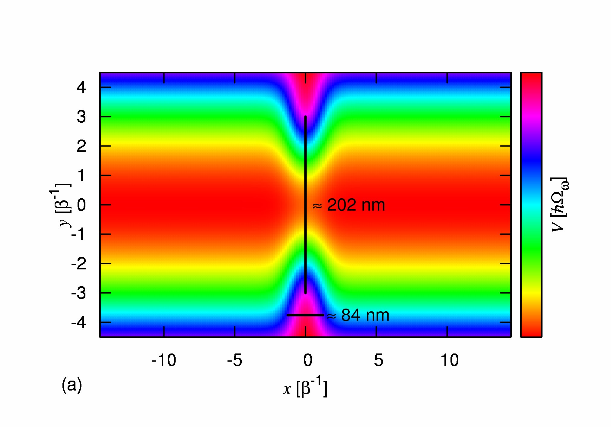
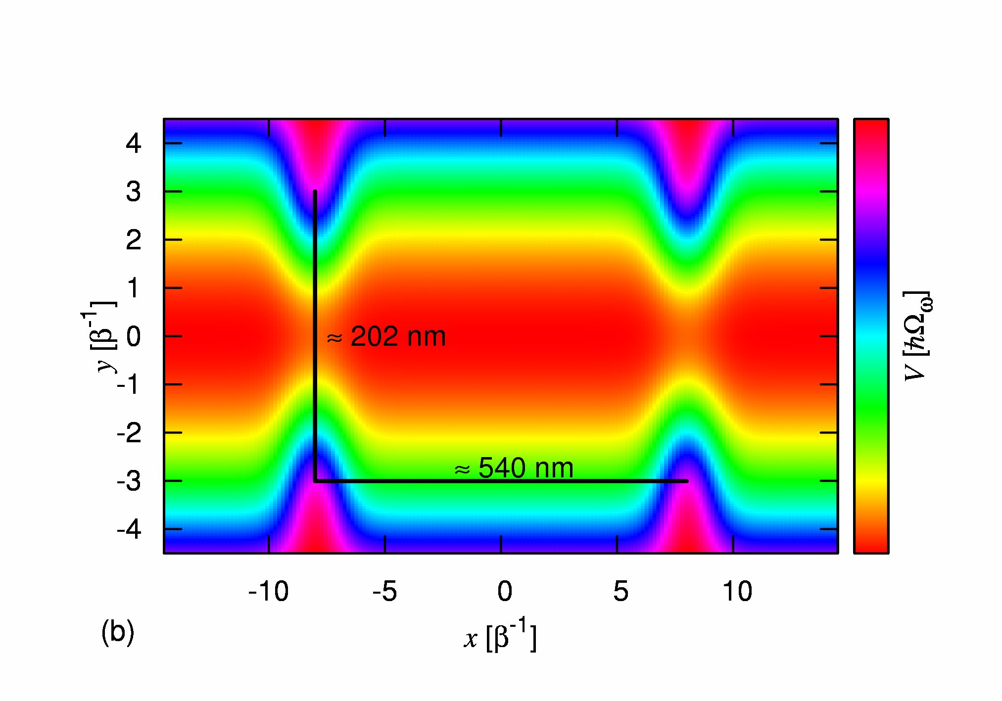
Figure 1: (Color online) Schematic diagram of gate-voltage controlled split-gate constriction with no magnetic field: (a) Sketch of a single split-gated quantum constriction; (b) Sketch of a double split-gated quantum constriction.

The considered single QPC (SQPC) system shown in Fig. 1(a) can be modeled by the Gaussian-shaped potential

$$V_{sc}(x,y) = V_{s}e^{-\alpha_{x}x^{2}-\alpha_{y}(y-y_{0})^{2}}$$ (21)

$$+ V_{s}e^{-\alpha_{x}x^{2}-\alpha_{y}(y+y_{0})^{2}}\,,$$

where $y_{0}$ is the distances of the Gaussian potential peak away from the center of the wire in the $\mathbf{y}$-direction. The parameters for the potential in Eq. (21) are $V_{s}=6.5$ meV, $\alpha_{x}=0.5\beta_{0}^{2}$, $\alpha_{y}=0.3\beta_{0}^{2}$, and $y_{0}=3\beta_{0}$ such that the width of the QPC is $84$ nm and the distance of the split-gates is approximately $202$ nm. The double QPC (DQPC) system shown in Fig. 1(b) is described using four Gaussian-shaped potentials

$$V_{sc}(x,y) = V_{s}e^{-\alpha_{x}(x-x_{0})^{2}-\alpha_{y}(y-y_{0})^{2}}$$ (22)

$$+ V_{s}e^{-\alpha_{x}(x+x_{0})^{2}-\alpha_{y}(y+y_{0})^{2}}$$

$$+ V_{s}e^{-\alpha_{x}(x-x_{0})^{2}-\alpha_{y}(y+y_{0})^{2}}$$

$$+ V_{s}e^{-\alpha_{x}(x+x_{0})^{2}-\alpha_{y}(y-y_{0})^{2}}\,,$$

where $(x_{0},y_{0})$ are the center coordinates of the Gaussian potentials. The parameters are the same as the Eq. (21) except for $x_{0}=8\beta_{0}$.

To investigate the electronic transport properties under a perpendicular magnetic field, we select the confinement parameter $\hbar\Omega_{0}=1$ meV. We assume that the quantum constriction is fabricated in a high-mobility GaAs-Al_xGa_1-xAs heterostructure such that the effective Rydberg energy $E_{\mathrm{Ryd}}=5.92$ meV and the Bohr radius $a_{\rm B}=9.79$ nm. Length parameters are scaled using the the effective magnetic length at zero magnetic field, referred to as $\beta_{0}^{-1}$ $(\approx 33.72\,\mathrm{nm})$ while energy is either fixed in $\mathrm{meV}$ or given in units of the effective confinement strength $\hbar\Omega_{\omega}$.

We start by considering a SQPC placed at $x=0$ between two electron reservoirs, as shown in Fig. 1(a). We assume that the QPC could be induced by metallic split-gates situated on the top of the heterostructure and can be treated as an open structure with distance $d_{\rm SG}\approx 202$ nm.

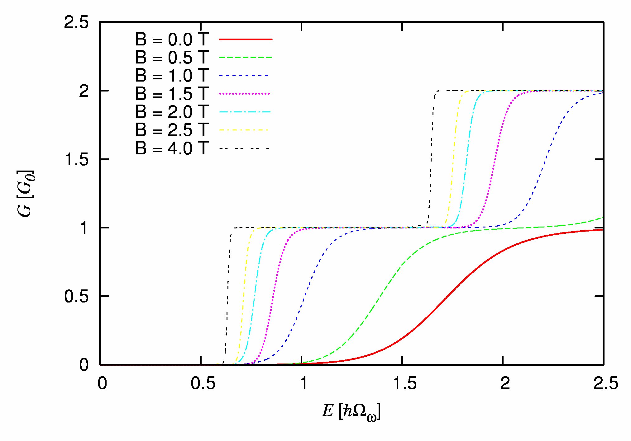
Figure 2: (Color online) Conductance through a single QPC as a function of energy under magnetic field with strength from 0.0 to 4.0 Tesla. The parameters of the constriction potentials are the same with Fig. 1(a).

In Fig. 2, we show the conductance as a function of incident energy under magnetic field. By increasing the magnetic field strength from $0.0$ to $4.0$ T, the subband threshold is red-shifted around $1.1\hbar\Omega_{\omega}$, and the pinch-off regime is also reduced. Moreover, for a given incident electron energy, increasing the magnetic field may enhance the conductance which tends to approach the ideal quantization. This is because of the formation of one-dimensional edge states in the channel suppressing the backscattering. Since there is no significant interference, we see that the conductance plateaus are monotonically increased as a function of energy for arbitrary magnetic fields implying that no AB oscillations could be induced in such a simple geometry and small source-drain bias regime.

To enhance the interference effects, we consider a DQPC made by two pairs of split-gates located at $x=\pm x_{0}$ with $x_{0}=8\beta_{0}$ [see Fig. 1(b)] forming a cavity with characteristic length $L\approx 540$ nm.

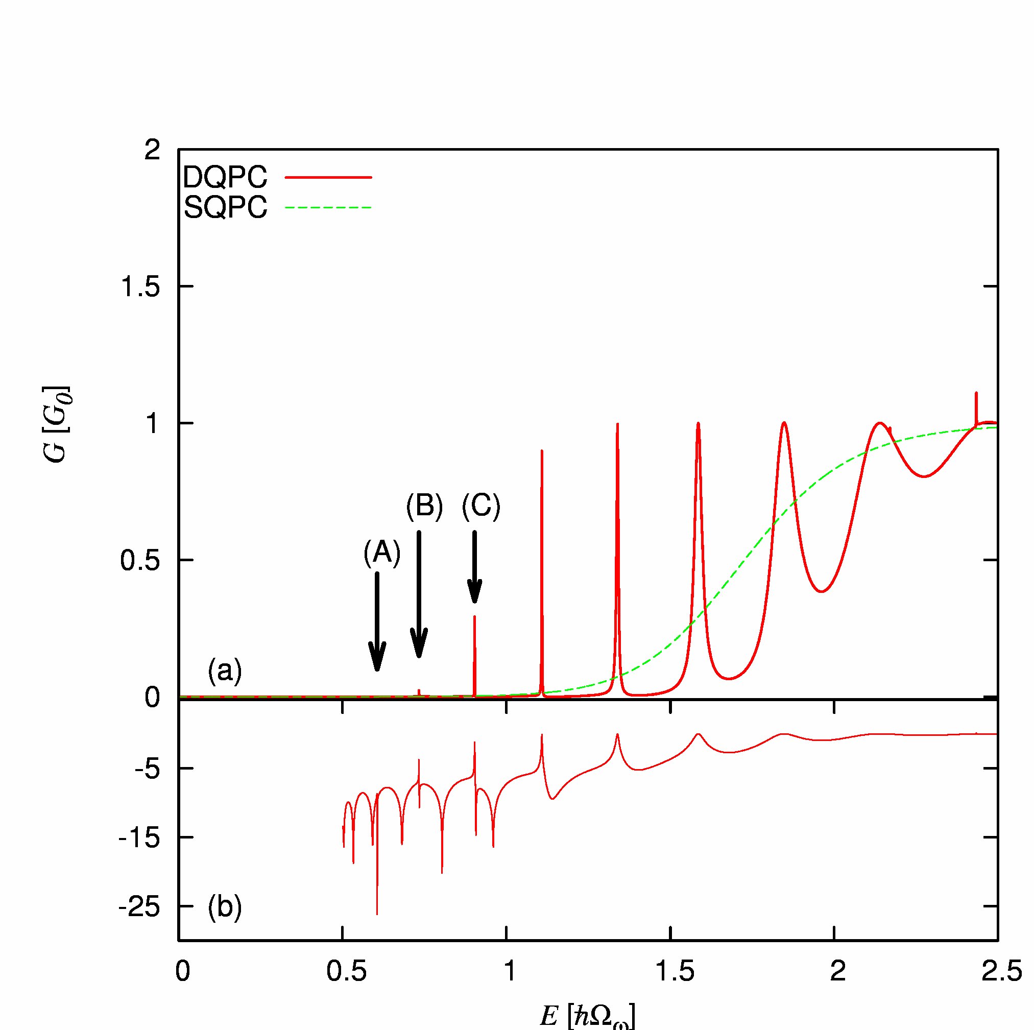
Figure 3: (Color online) Conductance as a function of energy with no magnetic field: (a) The conductance for the case of DQPC (red solid curve) in comparison with the case of SQPC (green dashed curve); (b) The logarithm conductance for the case of DQPC. The parameters for the potentials of the DQPC are the same as Fig. 1(b). The resonances (A)-(C) shown by the black arrows are at $E/\hbar\Omega_{\omega}=0.606$, $0.733$, and $0.903$.

In Fig. 3(a), we show the conductance as a function of incident energy in the DQPC system with no magnetic field (red solid curve) in comparison with the case of a SQPC (green dashed curve). By adding the second QPC, the conductance is strongly suppressed in the non-resonant energies. In addition, it is interesting to see that the conductance brings forth resonance peaks instead of dips.Tang et al. (2003) This implies that the QPC increases the subband threshold, so that electrons with energy in the pinch-off regime manifest resonant transmission feature induced by the cavity formed by the DQPC.

To obtain a deeper understanding for the resonance features shown by the black arrows in Fig. 3(a), we plot the logarithm conductance shown in Fig. 3(b). It is clearly seen that the resonance (A) manifests dip structure, while the resonances (B) and (C) exhibit the Fano line-shapes Fano (1961) indicating the interference between the localized and the extended states. Their corresponding probability densities are shown in Fig. 4(a)-(c).

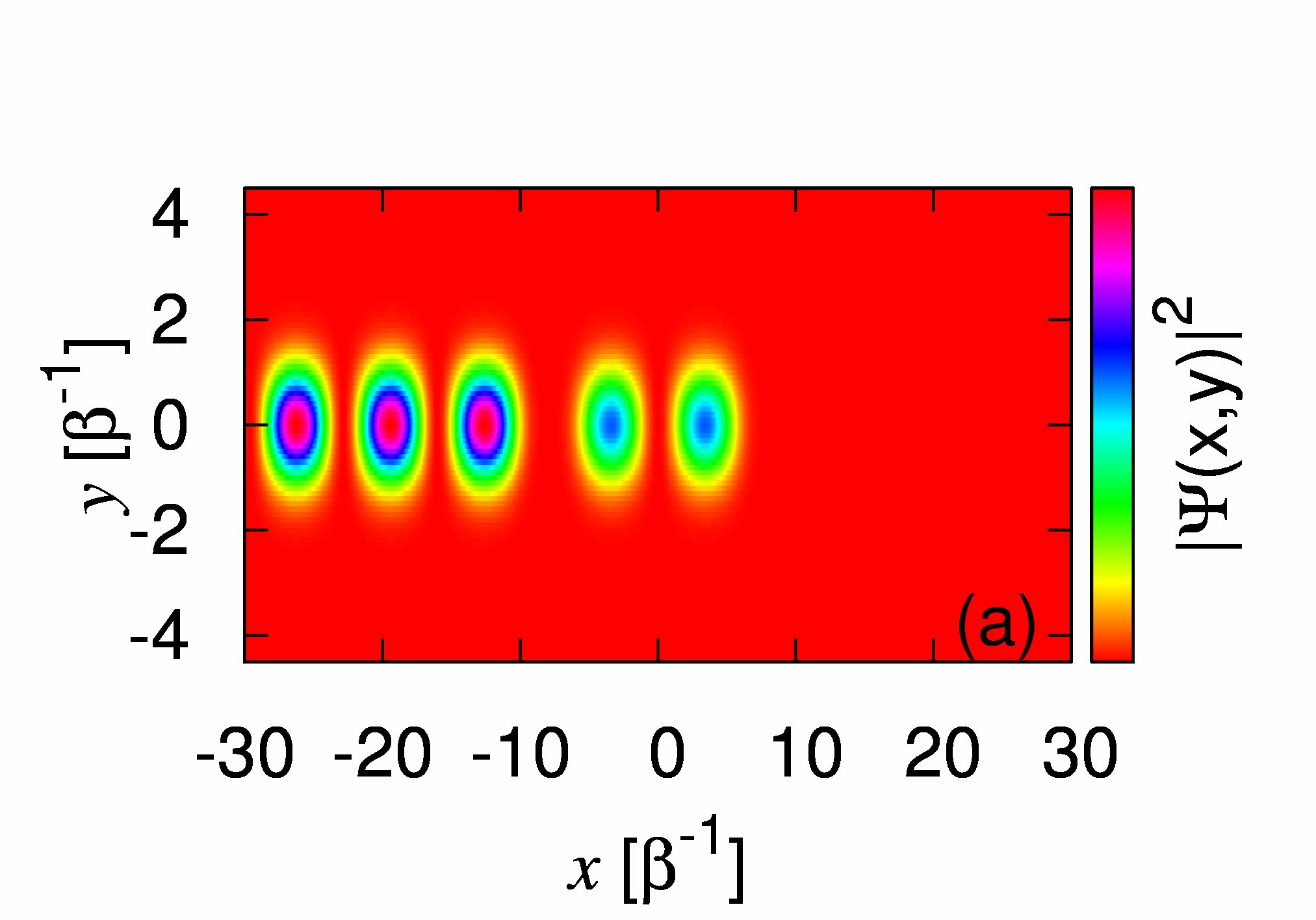
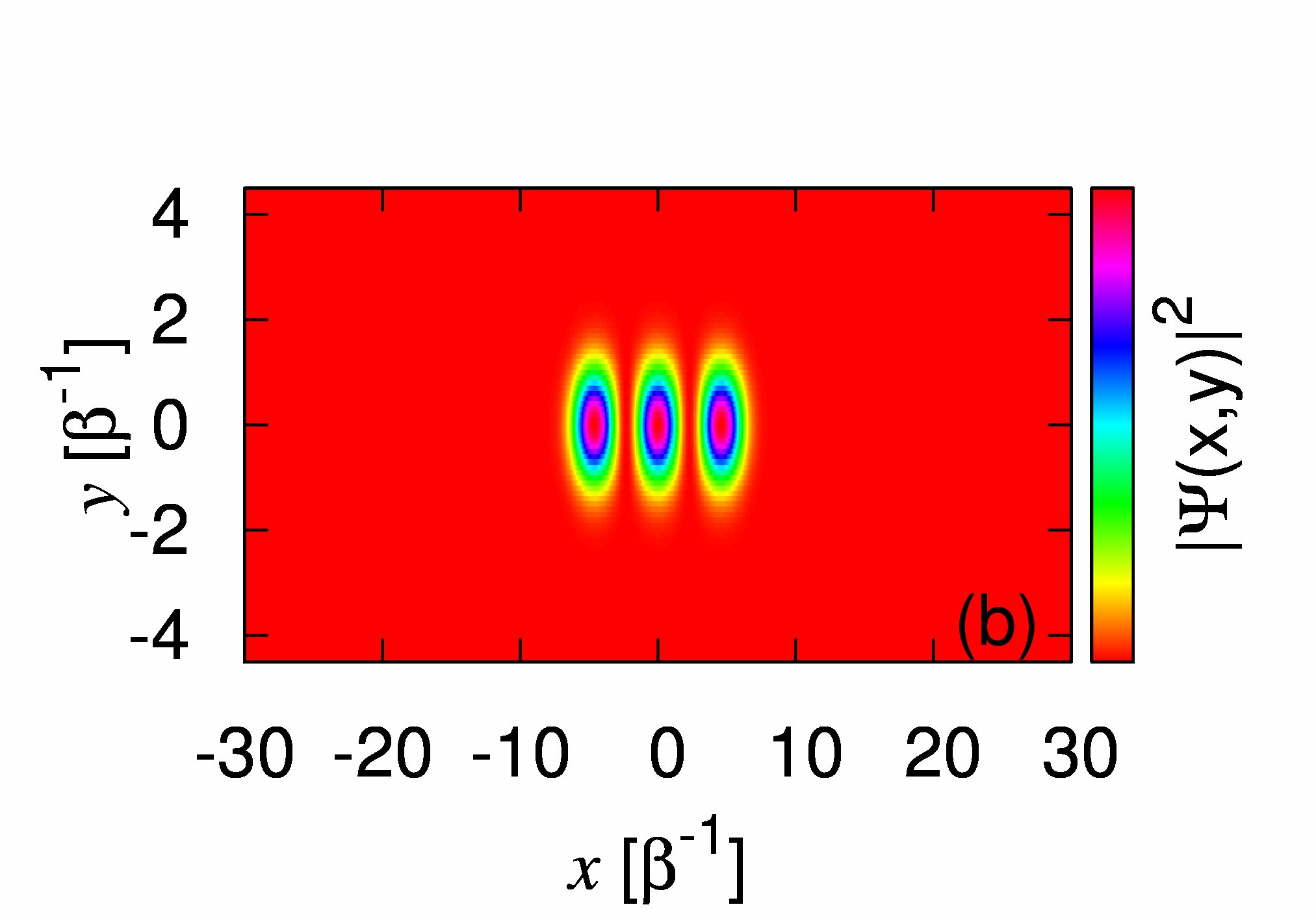
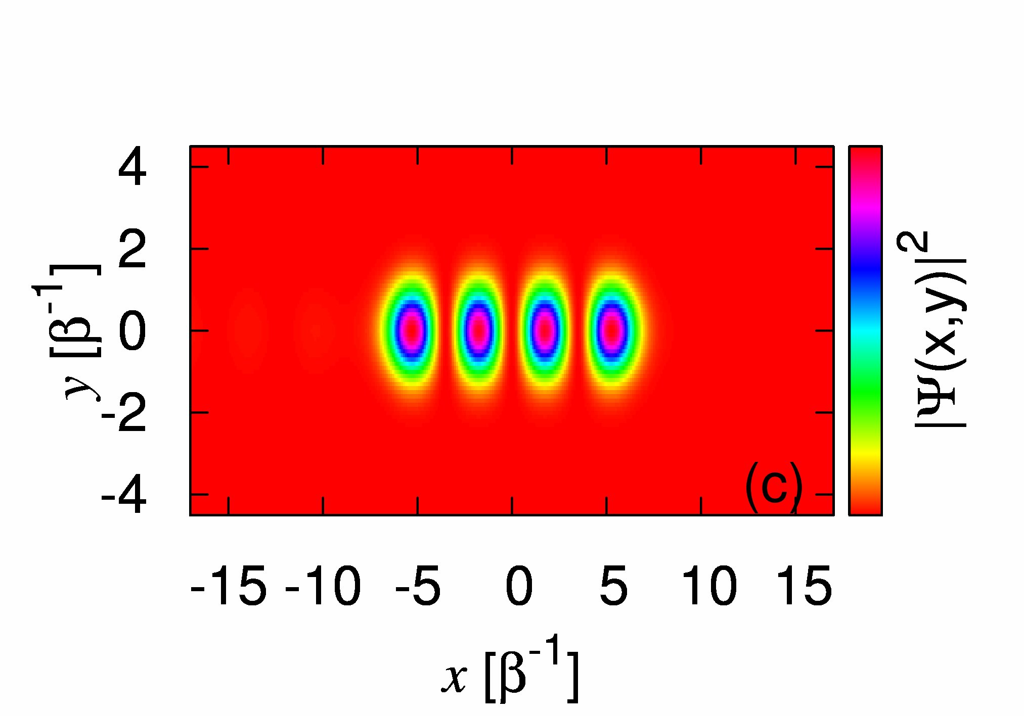
Figure 4: (Color online) Probability density for resonances in the conductance marked by (a)-(c) in Fig. 3(a) with corresponding energies $E/\hbar\Omega_{\omega}=$ (a) $0.606$; (b) $0.733$; (c) $0.903$.

The number of probability density peaks within the cavity region implies the order of the resonances formed in the cavity implying that the resonances (A)-(C) are the second to the fourth resonances in the cavity. The ratio of the distance between the nearby peaks to the incident wave length is around $2.0$, this indicates long-lived resonance modes fitting the cavity in the DQPC.

We now turn to study the magnetotransport properties in the split-gated systems.

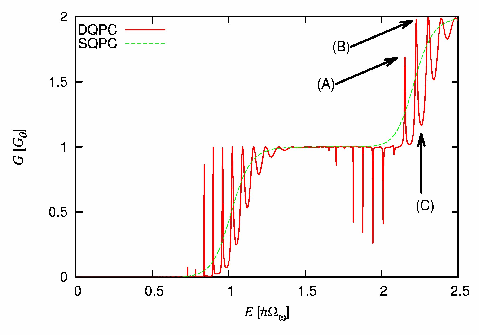
Figure 5: (Color online) Conductance as a function of energy with $B=1.0\,\mathrm{T}$. The other parameters are the same as previous figures.

In Fig. 5, we present abundant resonance features in conductance of SQPC (green dashed curve) and DQPC (red solid curve) under magnetic field $B=1.0$ Tesla. For the case of SQPC, the conductance is monotonically increased in the pinch-off regime ($E/\hbar\Omega_{\omega}<1.3$). The conductance quantization at $1.3<E/\hbar\Omega_{\omega}<2.0$ demonstrates that electrons can be transported coherently within the edge channel without significant backscattering. For the case of a DQPC, the conductance manifests resonant transmission peaks in the low kinetic energy regimes of the first and the second subbands, while the conductance exhibits resonant reflection features in the high kinetic energy regime. The resonance structures in the conductance are more dense due to the magnetic field.

To get a better understanding for the on- resonance peaks (A) and (B) as well as the off- resonance valley structure (C) marked by the black arrows in Fig. 5, we plot their corresponding probability densities in Fig. 6(a)-(c).

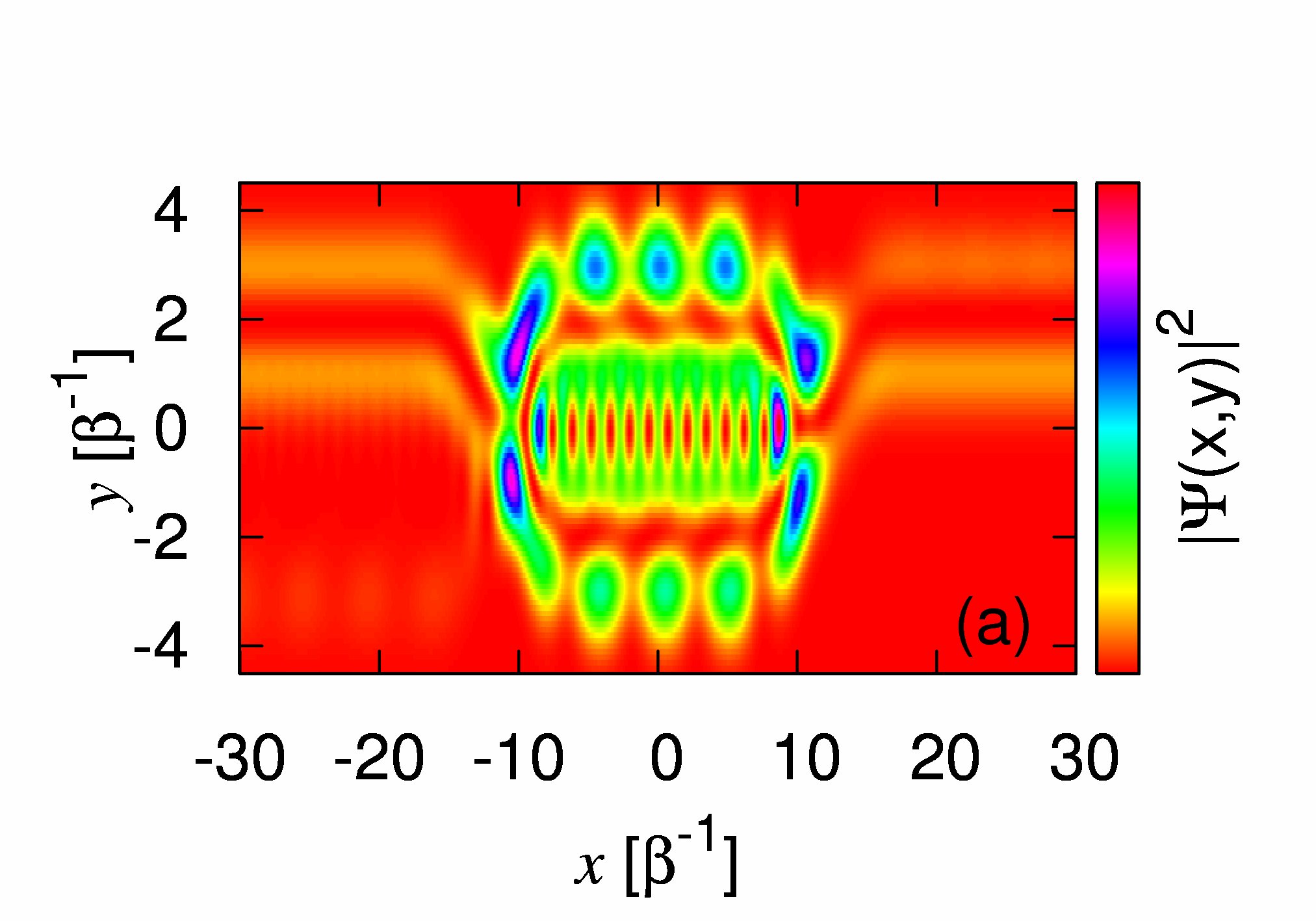
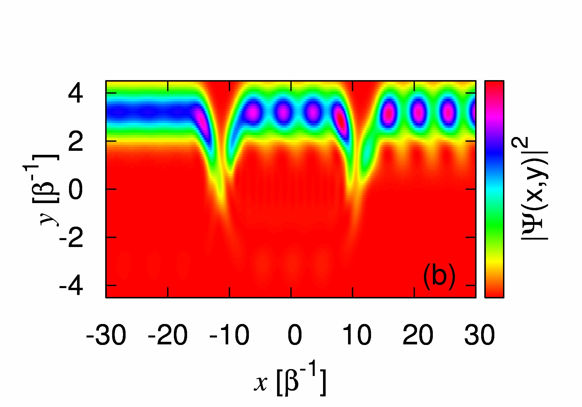
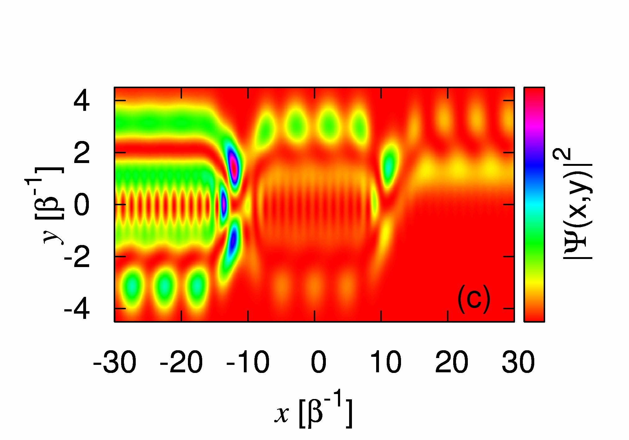
Figure 6: (Color online) Probability density for the peaks marked in Fig. 5. (a) A ring structure inside the cavity due to the magnetic field. $E/\hbar\Omega_{\omega}=2.152$, $n=1$. (b) An edge state. $E/\hbar\Omega_{\omega}=2.226$, $n=0$. (c) A scattering state. $E/\hbar\Omega_{\omega}=2.259$, $n=1$.

First, when the electron is transported with very low kinetic energy such as the case of Fig. 6(a) in which the electron is occupying the second subband $n=1$. We see that the localized states in the cavity can be well established forming double AB-oscillation paths, where the inner path manifests an entangled feature. In addition, the QBSs can be formed at both ends of the open cavity. Secondly, if the electron carries sufficient high kinetic energy such as the case of Fig. 6(b) in which the electron is occupying the first subband $n=0$. The Lorentz force plays a dominant role on the transport such that the electron wave is pushed to the upper confinement and forms an edge state facilitating the flow of electrons through the system by suppressing backscattering in the system. For comparison with the case (A), we show the non-resonance probability feature shown in Fig. 6(c) in which the electron is also occupying the second subband $n=1$. It is important that, in the non-resonant condition, the Lorentz force is able to push the electron a little bit to the upper confinement and QBS can be formed only at the left QPC thus manifesting reflection feature with minimal conductance.

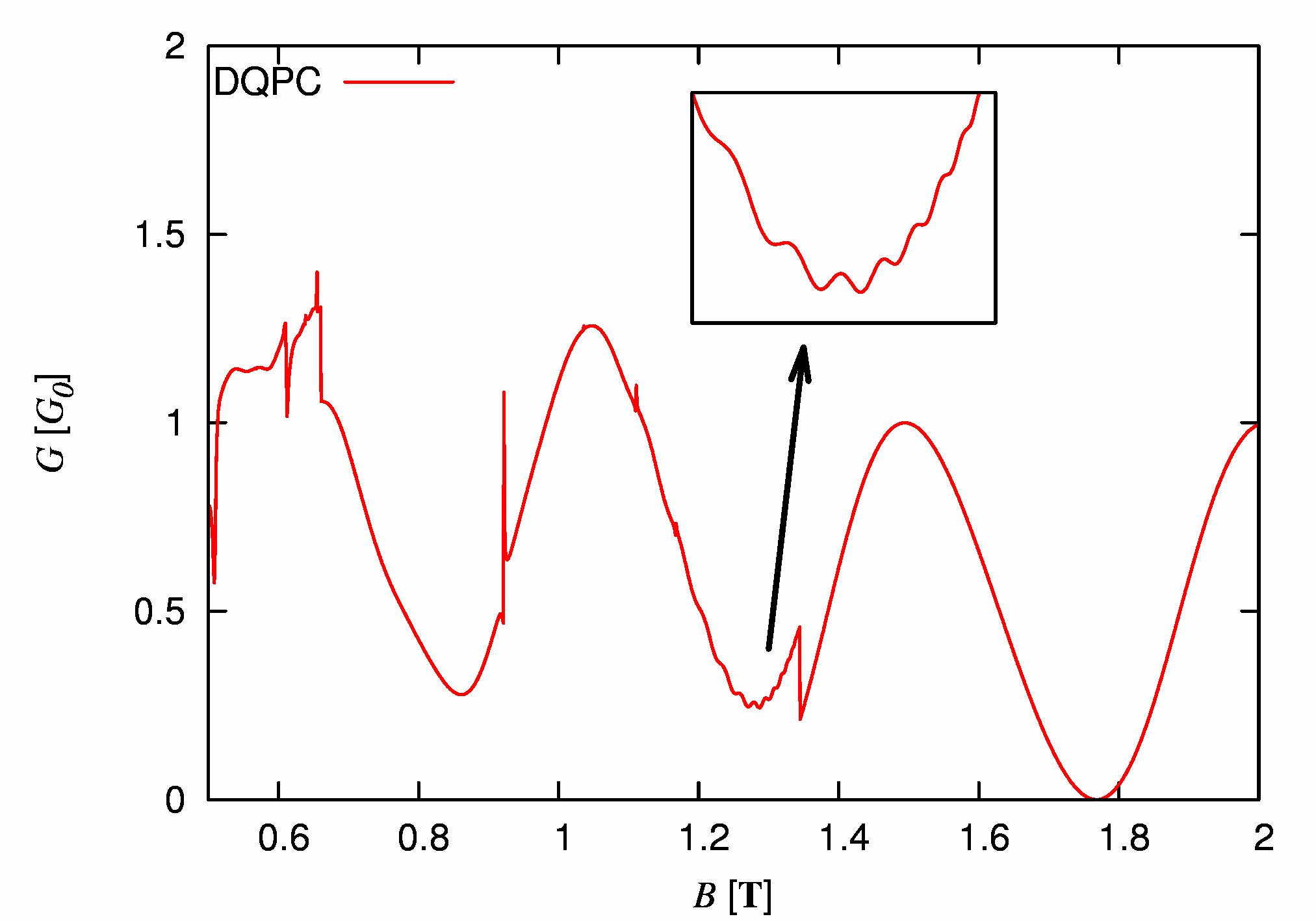
Figure 7: (Color online) Conductance $G$ as a function of magnetic field $B$ for electrons with incident energy $E/\hbar\Omega_{\omega}=1.9$ through DQPC. The inset shows that the conductance with small AB oscillations can be seen superimposed on large oscillations. The other parameters are $V_{s}=6.5\,\mathrm{meV}$, $\alpha_{x}=0.5\beta_{0}^{2}$, $\alpha_{y}=0.3\beta_{0}^{2}$, $y_{0}=3\beta_{0}$, and $x_{0}=8\beta_{0}$.

In Fig. 7, we show that the conductance versus magnetic field exhibits periodic oscillations. The period $\Delta B$ of AB oscillations is inversely proportional to the effective area ${\cal A}$ enclosed by the electron path, given by $\Delta B=\Phi_{0}{\cal A}^{-1}$ with $\Phi_{0}=h/e$ being the flux quantum. Ihnatsenka and Zozoulenko (2008) The effective area can be slightly changed by tuning the strength $V_{s}$ of split gates. The AB oscillations with large period $\Delta B\approx 0.5$ Tesla is associated with the interference between the directly reflected electrons by the left QPC and the electrons go through an enclosed path forming a small area in the left QPC (area I in Fig. 8). The small oscillations superimposed on the larger ones shown in the inset of Fig. 7 are formed due to the interference between the electrons directly reflected by the right QPC and the electrons going through the open cavity forming a large area in the DQPC (area II in Fig. 8).

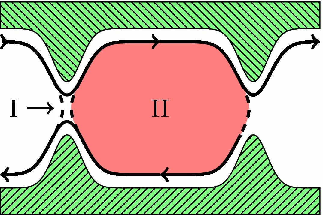
Figure 8: (Color online) Illustration of the possible paths that the electrons can take and the paths that they enclose in the DQPC system confined by double split gates (shaded regions).

We note in passing that our results demonstrate that the AB oscillations do not require a ring geometry. van Loosdrecht et al. (1988) Interference is the most important effect to generate AB oscillations. Moreover, the robust zero conductance feature at around $B\simeq 1.77$ Tesla exhibits that the DQPC could be applicable as a mesoscopic switching device.

To explore the time-dependent transport in a DQPC with time-harmonic modulation, we construct the model by using four Gaussian-shaped potentials that are expressed as

$$V_{sc}(x,y,t) = V_{\rm L}(t)e^{-\alpha_{x}(x-x_{0})^{2}-\alpha_{y}(y-y_{0})^{2}}$$ (23)

$$+ V_{\rm L}(t)e^{-\alpha_{x}(x+x_{0})^{2}-\alpha_{y}(y+y_{0})^{2}}$$

$$+ V_{\rm R}(t)e^{-\alpha_{x}(x-x_{0})^{2}-\alpha_{y}(y+y_{0})^{2}}$$

$$+ V_{\rm R}(t)e^{-\alpha_{x}(x+x_{0})^{2}-\alpha_{y}(y-y_{0})^{2}}\,,$$

where strengths of the left QPC $V_{\rm L}(t)=V_{s}+V_{t}\cos{\omega t}$ and the right QPC $V_{\rm R}(t)=V_{s}+V_{t}\cos{(\omega t+\phi_{0})}$ contain the same driving frequency $\omega$ with a phase difference $\phi_{0}$. This driven DQPC system is similar to the one depicted in Fig. 1(b) except for the external driving terms with amplitude $V_{t}$.

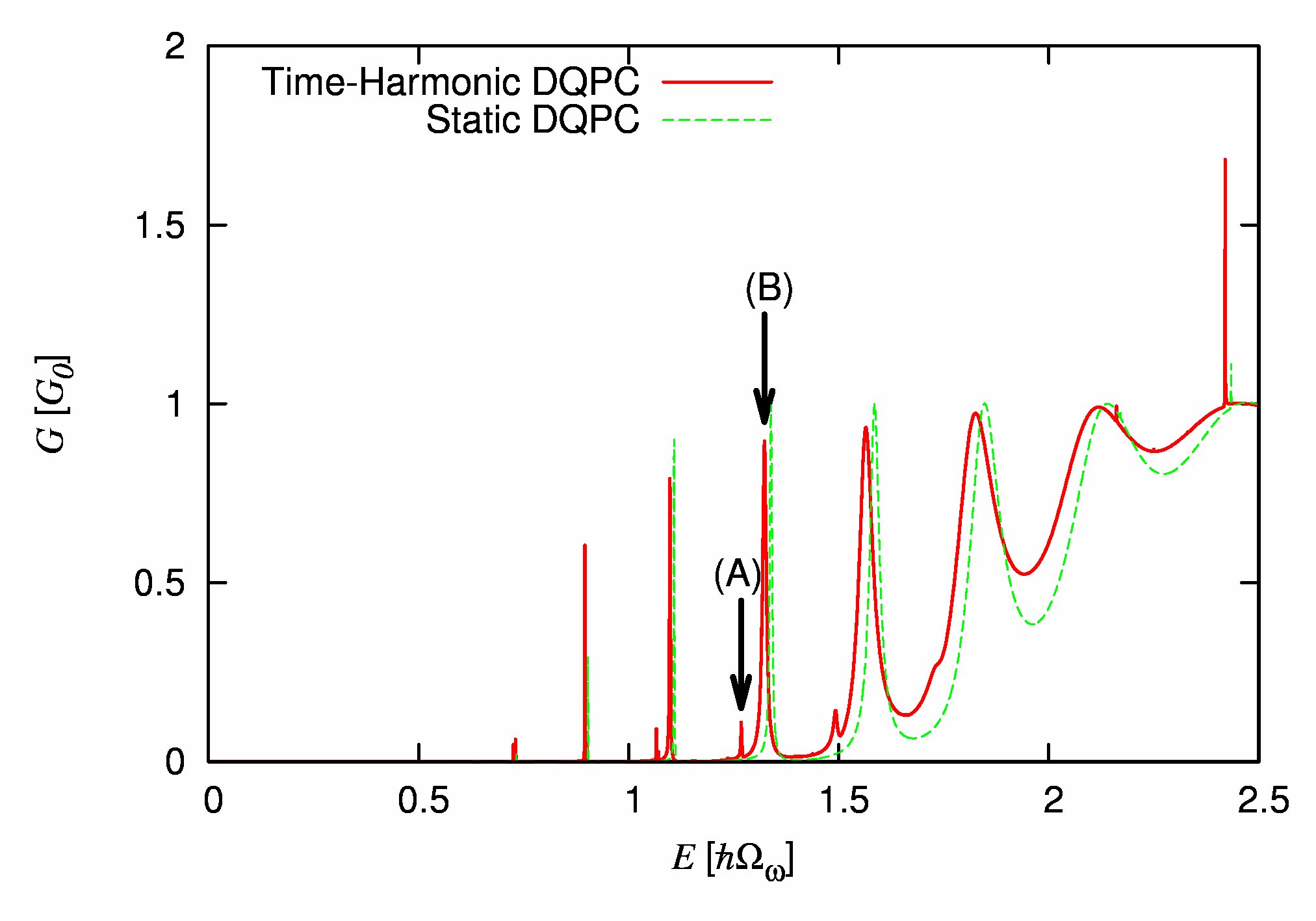
Figure 9: (Color online) Conductance versus incident energy with no magnetic field ($B=0$) for a time-harmonic DQPC ($V_{t}=0.5$ meV and $\phi_{0}=\pi$, red solid) in comparison with that of a static DQPC ($V_{t}=0.0$ meV, green dashed). The other parameters for the system are $V_{s}=6.0\,\mathrm{meV}$, $\alpha_{x}=0.5\beta_{0}^{2}$, $\alpha_{y}=0.3\beta_{0}^{2}$, $y_{0}=3\beta_{0}$, $x_{0}=8\beta_{0}$, and driving frequency $\omega=0.17\Omega_{\omega}$.

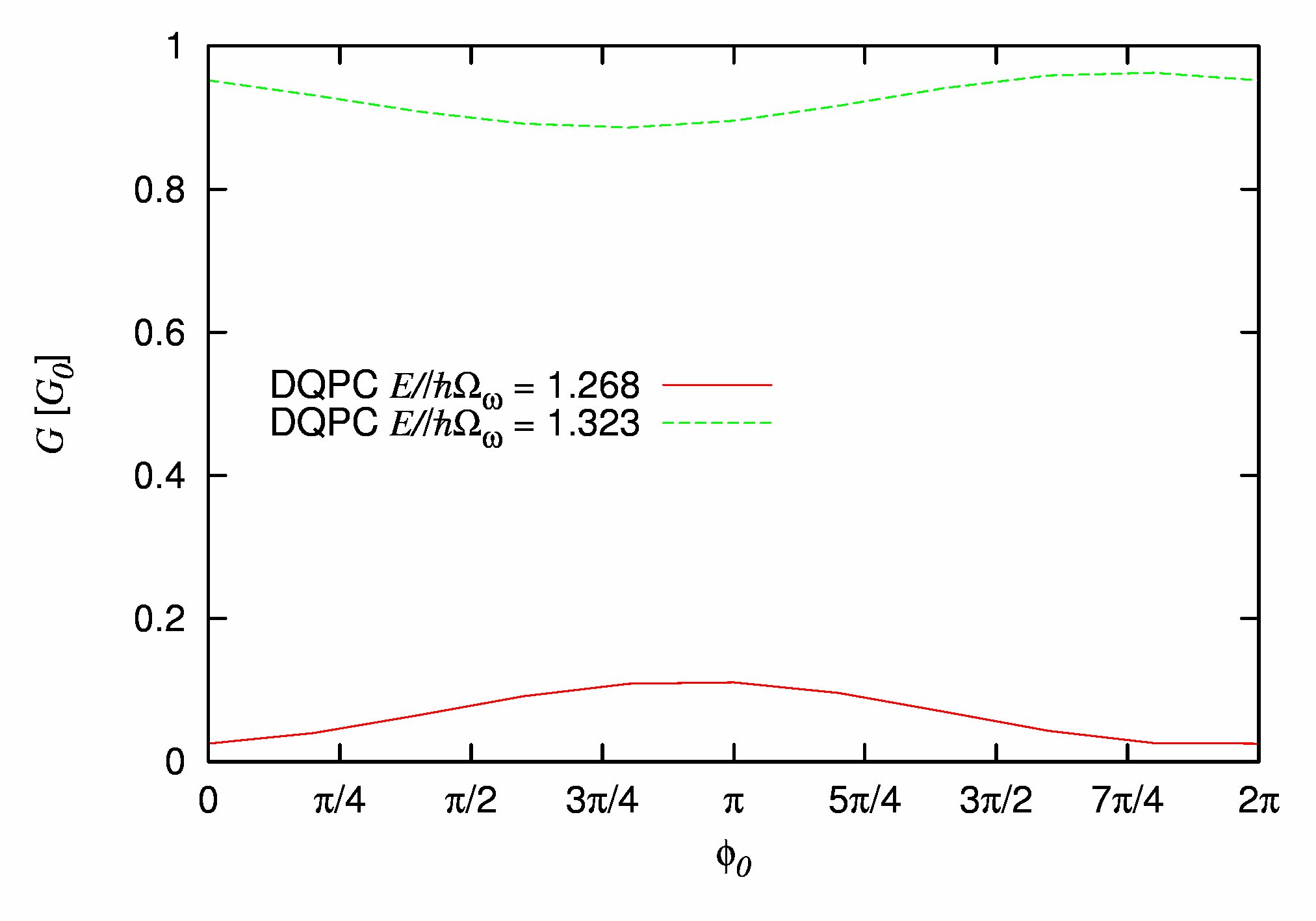
Figure 10: Conductance $G$ versus phase difference $\phi_{0}$ between the left and the right QPCs for the electron with energies marked by (A) and (B) in Fig. 9.

In Fig. 9, we show the conductance as a function of incident energy for the time-harmonic DQPC ($V_{t}=0.5$ meV and $\phi_{0}=\pi$, red solid curve) in comparison with the static DQPC ($V_{t}=0.0$ meV, green dashed curve). Under the influence of the time-harmonic driving potential, we find a small side peak in $G$ marked by (A) indicating that the electron is allowed to emit a photon with energy $\hbar\omega$ and jump to a state beneath the resonance, i.e., the main peak marked by (B). Moreover, the electron kinetic energy plays a role to suppress such inter-sideband transitions. As we can see that the small peak becomes a shoulder structure for an electron with incident energy at around $E\simeq 1.75\hbar\Omega_{\omega}$. In Fig. 10, we show the conductance as a function of phase difference between the two QPCs. The energies are fixed at the main peak $E=1.323\hbar\Omega_{\omega}$ (green dashed curve) and at the side peak $E=1.268\hbar\Omega_{\omega}$ (red solid curve) marked, respectively, by (A) and (B) in Fig. 9. Both cases are not very sensitive to the phase difference $\phi_{0}$, but we see that $\phi_{0}$ at around $\pi$ can enhance the inter-sideband transitions.

IV Concluding Remarks

We have developed a Lippmann-Schwinger model that has allowed us to explore the magnetotransport and time-dependent transport spectroscopy of coherent elastic and inelastic multiple scattering features relevant to quantum constricted SQPC and DQPC systems under a magnetic field perpendicular to the 2DEG. We have demonstrated and analyzed the mechanisms causing the slow and the fast conductance oscillations due to AB interference in the DQPC system. We hope that our numerical demonstrations on magnetotransport and time-dependent transport could be useful for the utilization of intricate coupling between subbands and sidebands towards the realization of quantum pumping circuits and fast manipulation of quantum information processing in mesoscopic systems.