Magnetic solitons in frustrated ferromagnetic spin chain

Abstract

We study the classical anisotropic ferromagnetic spin chain with frustration. The behavior of soliton and kink solutions in the vicinity of the ground state phase transition from the ferromagnetic to the spiral phase is studied. The dependence of the soliton energy on small anisotropy parameter is established using scaling estimates and numerical minimization of the energy functional. Conditions of the existence of the solitons are determined. It is shown that solitons survive in the spiral phase though with some restrictions on their size. A comparison of the energies of the classical solitons and the bound magnon complexes in the quantum model shows the functional similarity between them. The influence of the finite-size effects on the soliton states is studied and it is shown that the localized solitons originate from the uniform state when the system size exceeds some critical value depending on the anisotropy.

I Introduction

Lately, there has been considerable interest in low-dimensional spin systems that exhibit frustration review . A very interesting class of such systems is chain compounds consisting of edge-sharing $CuO_{4}$ units. Recently, a variety of these copper oxides were synthesized and found to show unique physical properties Mizuno ; Masuda ; Hase ; Capogna ; stefan05 ; stefan08 . The frustration in these compounds arises from the competition of exchange interactions between magnetic $Cu^{2+}$ ions carrying spins $1/2$. Due to a specific geometry of these systems ($Cu-O-Cu$ angle is close to $90^{0}$) the nearest-neighbor (NN) interaction is ferromagnetic, while the next-nearest-neighbor (NNN) one is antiferromagnetic and absolute values of these interactions are comparable Mizuno ; stefan08 . An appropriate model describing the magnetic properties of such copper oxides is so-called F-AF spin chain model the Hamiltonian of which has a form

$$H=J_{1}\sum_{n=1}^{N}(S_{n}^{x}S_{n+1}^{x}+S_{n}^{y}S_{n+1}^{y}+\Delta_{1}S_{n}^{z}S_{n+1}^{z})+J_{2}\sum_{n=1}^{N}(S_{n}^{x}S_{n+2}^{x}+S_{n}^{y}S_{n+2}^{y}+\Delta_{2}S_{n}^{z}S_{n+1}^{z})$$ (1)

where $J_{1}<0$ and $J_{2}>0$.

This model is characterized by a frustration parameter $\lambda=J_{2}/|J_{1}|$. The quantum F-AF $s=1/2$ model has been intensively studied last years Chubukov ; KO ; DK06 ; Vekua ; Lu ; DKR ; Itoi ; Kecke ; Laeuchli . Most of studies of this model are related to the isotropic case ($\Delta_{1}=\Delta_{2}=1$). It is known that the ground state of the isotropic model is ferromagnetic for $\lambda<1/4$. At $\lambda=1/4$ the phase transition to the incommensurate singlet phase with spiral spin correlations takes place. Remarkably, this transition point does not depend on spin value $s$ at $N\to\infty$. It was shown also that the F-AF $s=1/2$ model with anisotropic interactions has a rich phase diagram Somma . In our papers DK08 ; DK09 we investigated weakly anisotropic ($\Delta_{1}>1$, $\Delta_{2}=1$) quantum spin-1/2 model (1). It was shown that even small anisotropy essentially effects on the properties of the model. In particular, the transition point from the ferromagnetic to the spiral-like ground state shifts from $\lambda=1/4$.

An interesting feature of the quantum anisotropic model (1) is the existence of the multimagnon bound complexes in the ferromagnetic phase. These complexes govern the low-temperature thermodynamics DK09 ; Johnson . It was noted also that the NNN interaction strongly affects the excitation spectrum especially in the vicinity of the transition point $\lambda=1/4$.

It is known that there is a close relation between the multimagnon bound complexes in the quantum spin models and soliton and kink excitations in the classical counterparts. In particular, these soliton states have been studied extensively for the classical easy-axis ferromagnetic chain and a connection between them and the bound magnon complexes in the quantum $s=1/2$ model (1) at $J_{2}=0$ was discussed Schneider . On the other hand, the influence of the frustration on the solitons has not been considered before. The F-AF model represents a suitable model to study this problem and to investigate the connection between the quantum excitation spectrum and the soliton solutions of the classical frustrated spin model.

In DK08 we showed that the ground state phase diagram of the quantum model (1) with both $\Delta_{1}\neq 1$ and $\Delta_{2}\neq 1$ are qualitatively similar to that for the model with the anisotropy of the NN interaction only. Therefore, for simplicity we consider model (1) with $\Delta_{1}=\Delta>1$ and $\Delta_{2}=1$. In this case model (1) takes the form

$$H=-\sum\left(S_{n}^{x}S_{n+1}^{x}+S_{n}^{y}S_{n+1}^{y}+\Delta S_{n}^{z}S_{n+1}^{z}-\Delta s^{2}\right)+\lambda\sum(\mathbf{S}_{n}\cdot\mathbf{S}_{n+2}-s^{2})$$ (2)

where we put $|J_{1}|$ as an energy unit and added constant shifts to secure the energy of the ferromagnetic state to be zero.

The phase diagram of the classical F-AF model with $\Delta>1$ consists of the ferromagnetic and the spiral phases. The ferromagnetic ground state is simple, i.e., it has all spins parallel to the Z axis. However, the soliton excitations in this phase are not trivial especially near the transition point between the phases. Our main goal is to study the behavior of the solitons in the vicinity of the isotropic transition (IT) point ($\Delta=1$, $\lambda=1/4$) and to compare it with the properties of the excitations of the quantum model. As it will be shown the frustration effects strongly modify the soliton states especially for small anisotropy. In particular, the exponent characterizing the power dependence of the gap (the soliton energy with respect to the ground state) on the anisotropy is different from that for $\lambda=0$.

The paper is organized as follows. In Sec.II we represent the known results for soliton solutions of the anisotropic ferromagnetic chain (model (2) at $\lambda=0$). In Sec.III we consider the classical continuum F-AF model in the vicinity of the ground state phase transition from the ferromagnetic to the spiral phase. We deduce the corresponding energy functional and establish the scaling form of the soliton energy as a function of the anisotropy and the frustration parameter. In this section we also obtain asymptotes of the soliton solutions at large distances and determine the necessary conditions of the soliton stability. In Sec.IV we present results of the numerical minimization of the energy functional which confirm the scaling estimations. In Sec.V we study the finite-size effects on the soliton solution. In Sec.VI we show that the behavior of both classic solitons and $m$-magnon quantum spin excitations are functionally similar to $m$-boson bound complexes of the Bose model with the attractive interaction if $m$ is not large. In Sec.VII we give a summary of results.

II Classical model for $\lambda=0$ case

In the classical approximation the spin operators $\mathbf{S}_{n}$ are replaced by the classical vectors $\overrightarrow{S}_{n}$ of the fixed length $s$ which are parameterized by spherical coordinates

$$\overrightarrow{S}_{n}=s(\cos\varphi_{n}\sin\theta_{n},\sin\varphi_{n}\sin\theta_{n},\cos\theta_{n})$$ (3)

In terms of the angles $\theta_{n}$ and $\varphi_{n}$ the discrete classical F-AF model (2) takes the form

$$E = s^{2}\sum\left\{[1-\cos(\theta_{n+1}-\theta_{n})]-\lambda[1-\cos(\theta_{n+2}-\theta_{n})]+\alpha[1-\cos(\theta_{n+1})\cos(\theta_{n})]\right\}$$ (4)

$$+s^{2}\sum\left\{[1-\cos(\varphi_{n+1}-\varphi_{n})]\sin\theta_{n}\sin\theta_{n+1}-\lambda[1-\cos(\varphi_{n+2}-\varphi_{n})]\sin\theta_{n}\sin\theta_{n+2}\right\}$$

where $\alpha=\Delta-1>0$.

In this Section we briefly review the known results for the classical Heisenberg ferromagnetic chain with an easy-axis anisotropy, i.e., model (4) with $\lambda=0$. In this case the model is exactly solved in the continuum limit Steiner ; KIK .

The continuum limit of the classical model assumes that the vectors $\overrightarrow{S}_{n}$ can be replaced by the classical vector field $\overrightarrow{S}(x,t)$ with slowly varying orientations, so that

$$\overrightarrow{S}_{n+1}-\overrightarrow{S}_{n}\approx\frac{\partial\overrightarrow{S}(x_{n})}{\partial x}$$ (5)

where the lattice constant is chosen as unit length. The direction of the vector field $\overrightarrow{S}(x,t)$ is determined by two angular variables $\varphi(x,t)$ and $\theta(x,t)$ according to Eq.(3).

The dynamics of the vector field $\overrightarrow{S}(x,t)$ is governed by the Landau-Lifshitz equation:

$$-\frac{\partial\overrightarrow{S}}{\partial t}=\overrightarrow{S}\mathbf{\times}\frac{\delta E}{\delta\overrightarrow{S}}$$ (6)

where we put $\hbar=1$. Here $E$ is the energy as a functional of the vector field $\overrightarrow{S}(x,t)$. Using the continuum approximation (5), Hamiltonian (2) goes over into the well-known energy functional:

$$E=\int\mathrm{d}x\left[\frac{1}{2}\left(\frac{\partial\overrightarrow{S}}{\partial x}\right)^{2}+\alpha\left(s^{2}-S_{z}^{2}\right)\right]$$ (7)

Classical equation of motion (6) for model (7) has two constants of the motion: the magnetization (continuum analog to a number of magnons)

$$M=s\int\mathrm{d}x(1-\cos\theta)$$ (8)

where we subtract a constant to make $M$ finite for solitons, and the momentum

$$P=s\int\mathrm{d}x(1-\cos\theta)\frac{\partial\varphi}{\partial x}$$ (9)

The ground state of (7) is the ferromagnetic configuration with all spins parallel (or antiparallel) to the Z axis, i.e. $\theta=0$ ($\theta=\pi$). The soliton configurations are specified by the boundary conditions $\theta\to 0$ ($\theta\to\pi)$ at $x\to\pm\infty$.

Fortunately, the classical equations of motion (6) for model (7) are exactly solvable Laksh . In particular, the energy for a given values of $M$ and $P$ is

$$E_{M,P}(\alpha)=4s^{2}\sqrt{2\alpha}\frac{\cosh(M\sqrt{2\alpha}/2s)-\cos(P/2s)}{\sinh(M\sqrt{2\alpha}/2s)}$$ (10)

Remarkably, Eq.(10) reproduces the exact result for the energy at $\alpha\ll 1$ of the $M$-magnon bound state Ovchinnikov for the most quantum case $s=1/2$.

Here we will show that simple scaling arguments are able to establish the correct scaling dependence for the energy. For this aim we rescale the coordinate $x=\xi/\alpha^{1/2}$ and introduce the normalized spin vector field $\overrightarrow{n}(x,t)=\overrightarrow{S}(x,t)/s$ in Eq.(7), which results in

$$E=s^{2}\alpha^{1/2}\int\mathrm{d}\xi\left[\frac{1}{2}\left(\frac{\partial\overrightarrow{n}}{\partial\xi}\right)^{2}+(1-n_{z}^{2})\right]$$ (11)

We notice that the integrand in equation (11) does not depend on any parameters and is expressed through the normalized spin vector field. This means that the energy scales as $E\sim s^{2}\alpha^{1/2}$, which is correct for a kink or for a large soliton excitations (see Eq.(10)). However, we can make one more step. The same procedure for magnetization (8) gives

$$M=s\alpha^{-1/2}\int\mathrm{d}\xi(1-n_{z})$$ (12)

This expression means that the magnetization forms a scaling parameter $M\alpha^{1/2}/s$. In a similar manner one can find that momentum (9) produces a dimensionless parameter $P/s$ independent of $\alpha$.

Thus, the energy of a soliton of the size $M$ having a momentum $P$ can be written in a form:

$$E=s^{2}\alpha^{1/2}f(M\alpha^{1/2}/s,P/s)$$ (13)

where $f$ is a scaling function, which can not be found in the framework of this scaling estimate. Fortunately, for model (7) this function is known exactly (10), which validates the above scaling arguments. Thus, simple scaling estimates allowed us to establish the scaling parameters and the scaling form for the soliton energy.

There is one more important fact which is worth noting here. The exact static solution for a kink in the discrete XXZ model with classical spins has been constructed by Gochev in Ref.gochev . He found that the kink energy has a form

$$E_{\mathrm{kink}}=2s^{2}\sqrt{\Delta^{2}-1}$$ (14)

which reproduces the exact result for the case $s=1/2$ Ovchinnikov . This allows us to assume that the energy of kink (or large soliton, which has double energy of kink) for XXZ chain with any value of $s$ has an universal dependence on $\Delta$ (14). We will see that this universality is destroyed in case $\lambda\neq 0$.

III Classical continuum spin model near the IT point

The NNN term in model (2) causes the frustration in the system and immediately destroys the integrability of the model. However, the behavior of the system for $0<\lambda<1/4$ and weak easy-axis anisotropy remains very similar to the case $\lambda=0$. In the classical and continuum approximation the Hamiltonian reduces to an energy functional (7) with renormalized factor $(1-4\lambda)/2$ at $(\partial\overrightarrow{S}/\partial x)^{2}$. In particular, this means that the found scaling form for the soliton energy (13) remains valid.

The situation drastically changes near the IT point ($\lambda=1/4,\ \Delta=1$) where the ground state phase transition in the isotropic case takes place. Let us deduce the energy functional describing the vicinity of this point. The continuum approximation assumes that the differences $(\theta_{n+1}-\theta_{n})$ and $(\varphi_{n+1}-\varphi_{n})$ are small and Eq.(4) can be expanded in these differences. However, in the vicinity of the IT point it is more clear and instructive to derive the continuum approach in terms of a spin vector field. For this aim we rewrite Hamiltonian (2) in the form:

$$H=\frac{1}{8}\sum(\mathbf{S}_{n+1}-2\mathbf{S}_{n}+\mathbf{S}_{n-1})^{2}-\frac{\gamma}{8}\sum(\mathbf{S}_{n+1}-\mathbf{S}_{n-1})^{2}+\alpha\sum(s^{2}-S_{n}^{z}S_{n+1}^{z})$$ (15)

where the parameters $\alpha=\Delta-1$ and $\gamma=4\lambda-1$ are small in the vicinity of the IT point.

In the classical and the continuum approach the expression containing spin operators in the first term in Eq.(15) is replaced by

$$\overrightarrow{S}_{n+1}-2\overrightarrow{S}_{n}+\overrightarrow{S}_{n-1}\approx\frac{\partial^{2}\overrightarrow{S}(x_{n})}{\partial x^{2}}$$ (16)

and that in the second term in Eq.(15) according to Eq.(5).

Thus, Hamiltonian (15) is mapped to the energy functional

$$E=\int\mathrm{d}x\left[\frac{1}{8}\left(\frac{\partial^{2}\overrightarrow{S}}{\partial x^{2}}\right)^{2}-\frac{\gamma}{2}\left(\frac{\partial\overrightarrow{S}}{\partial x}\right)^{2}+\alpha\left(s^{2}-S_{z}^{2}\right)\right]$$ (17)

The effect of the fourth-order term $(\partial^{2}\overrightarrow{S}/\partial x^{2})^{2}$ in the energy functional like (17) was studied before ivanov , but it was considered as a small correction to the main contribution given by the term $(\partial\overrightarrow{S}/\partial x)^{2}$. On the contrary for our model (17) near the IT point the fourth-order term $(\partial^{2}\overrightarrow{S}/\partial x^{2})^{2}$ becomes the leading one. The appearance of the fourth-order term is related to the fact that the one-magnon spectrum in the IT point becomes $\varepsilon(k)\sim k^{4}$.

The energy functional (17) in terms of the angular variables $\varphi(x)$ and $\theta(x)$ has a rather cumbersome form:

$$E = \frac{s^{2}}{8}\int\mathrm{d}x\left[\theta^{\prime\prime 2}+\theta^{\prime 4}-4\gamma\theta^{\prime 2}+(\varphi^{\prime\prime 2}+\varphi^{\prime 4}-4\gamma\varphi^{\prime 2}+8\alpha)\sin^{2}\theta\right]$$ (18)

$$+\frac{s^{2}}{8}\int\mathrm{d}x\left[(4-2\sin^{2}\theta)\varphi^{\prime 2}\theta^{\prime 2}+(2\varphi^{\prime\prime}\varphi^{\prime}\theta^{\prime}-\varphi^{\prime 2}\theta^{\prime\prime})\sin(2\theta)\right]$$

where the prime denotes the space derivatives $\partial/\partial x$. One can check that Eq.(18) represents the leading terms in the expansion of Eq.(4) in small differences $(\theta_{n+1}-\theta_{n})$ and $(\varphi_{n+1}-\varphi_{n})$, which is actually assumed in the continuum approximation.

At first, let us study the phase diagram of the classical continuum model (18). Numerical calculations (details will be given below) confirmed a natural assumption that the ground state spin configuration for the easy-axis anisotropy case ($\alpha>0$) corresponds to the choice $\varphi=\mathrm{const}$. In this case the energy functional (18) simplifies to

$$E=\frac{s^{2}}{8}\int\mathrm{d}x(\theta^{\prime\prime 2}+\theta^{\prime 4}-4\gamma\theta^{\prime 2}+8\alpha\sin^{2}\theta)$$ (19)

Variation of the energy functional (19) in $\theta(x)$ leads to the Euler equation

$$\frac{1}{4}\theta^{\prime\prime\prime\prime}-\frac{3}{2}\theta^{\prime\prime}\theta^{\prime 2}+\gamma\theta^{\prime\prime}+\alpha\sin(2\theta)=0$$ (20)

The ground state in the ferromagnetic phase has a trivial solution $\theta=0$ (or $\theta=\pi$) with zero energy. In the isotropic case ($\alpha=0$) the transition from the ferromagnetic to the spiral phase takes place at $\lambda=1/4$. For $\lambda>1/4$ the solution $\theta(x)$ has a pure spiral form

$$\theta_{sp}(x)=\pm\sqrt{2\gamma}x$$ (21)

which evidently has zero mean spin projection on any axis $\left\langle S_{x,y,z}\right\rangle=0$ and describes the spiral in the XZ plane.

In the anisotropic case the spiral function (21) does not satisfy Eq.(20). However, it represents a good approximation for the solution in the spiral phase. Using this function as a variational one for the energy functional (19) we find that the transition between the ferromagnetic and the spiral phases occurs on the line $\gamma=\sqrt{\alpha}$.

Assuming that the correction to the spiral solution $\theta_{sp}(x)$ is small, we found from Eq.(20) that the first correction has the oscillating form:

$$\theta(x)\approx\sqrt{2\gamma}x-\frac{\alpha}{32\gamma^{2}}\sin(\sqrt{8\gamma}x)$$ (22)

This function is not a pure spiral: due to the oscillating correction the spin vectors prefer to direct along the Z axis, so that $\left\langle S_{z}^{2}\right\rangle>\left\langle S_{x}^{2}+S_{y}^{2}\right\rangle$. However the mean values of all total projections remain zero: $\left\langle S_{x,y,z}\right\rangle=0$.

The calculation of the energy functional (19) with the function (22) yields

$$\frac{E_{sp}}{s^{2}N}\approx-\frac{\gamma^{2}-\alpha}{2}-\frac{\alpha^{2}}{128\gamma^{2}}$$ (23)

One can see that the correction to the energy is really small in the spiral phase region. Energy (23) becomes negative for $\gamma\gtrsim 0.992\sqrt{\alpha}$. This means that taking the correction in Eq.(22) into account shifts the transition line from the ferromagnetic to the spiral phase on the value less than $1\%$ (the smallness of the correction in Eq.(22) allows us to leave the name spiral for this phase). The phase transition from the ferromagnetic to the spiral phase at $\gamma\approx 0.992\sqrt{\alpha}$ is obviously the first order one. The transition line $\gamma=0.992\sqrt{\alpha}$ is shown in Fig.1.

It is worth noting here that the found behavior of the transition line corresponds to the classical version of spin model (2) and it is shifted for the quantum spin-$s$ model. Quantum corrections for $s\geq 1$ change numerical coefficient in Eq.(23). But for the $s=1/2$ case they lead to another form of the transition line: $\gamma\sim\alpha^{3/5}$ DK08 .

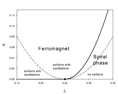
Figure 1: The phase diagram of the classical F-AF model. Thick line is the phase boundary between the ferromagnetic and the spiral phases. Dashed lines are boundaries between regions of different asymptotic regimes for large static solitons.

Now let us study the excitations of model (17). Similar to the case $\lambda=0$ the lowest configuration in the ferromagnetic region for a given $\left\langle S_{z}\right\rangle$ is described by the static soliton-like solutions of Eq.(20) with $\varphi=\mathrm{const}$ over the ferromagnetic configuration $\theta=0$ (or $\theta=\pi$). Unfortunately, we could not find the exact soliton solution near the IT point. However, it is possible to determine the scaling dependence of the energy of soliton of size $M$ on parameters $\alpha$ and $\gamma$ using scaling estimates as we did for the case $\lambda=0$. Near the IT point we perform the rescaling $x=\xi/\alpha^{1/4}$ and $\overrightarrow{S}(x,t)=s\overrightarrow{n}(x,t)$ which transforms the energy functional (17) to

$$E=s^{2}\alpha^{3/4}\int\mathrm{d}\xi\left[\frac{1}{8}\left(\frac{\partial^{2}\overrightarrow{n}}{\partial\xi^{2}}\right)^{2}-\frac{\mu}{2}\left(\frac{\partial\overrightarrow{n}}{\partial\xi}\right)^{2}+\left(1-n_{z}^{2}\right)\right]$$ (24)

with $\mu=\gamma/\sqrt{\alpha}$.

Since the integrand in Eq.(24) depends on the parameter $\mu$ only, we conclude that the energy of a kink or of a large soliton is $E=s^{2}\alpha^{3/4}f(\mu)$. As a result of rescaling the magnetization (8) becomes:

$$M=s\alpha^{-1/4}\int\mathrm{d}\xi(1-n_{z})$$ (25)

So, the magnetization produces a scaling parameter $\nu=\alpha^{1/4}M/s$. The momentum (9) forms the same parameter $k=P/s$ as for the case $\lambda=0$.

Thus, the energy of a soliton of the size $M$ can be represented in a form:

$$E=s^{2}\alpha^{3/4}f(\mu,\nu,k)$$ (26)

where the scaling function $f$ can be found numerically. This scaling form is exactly the same as was found for the quantum spin-$1/2$ model near the IT point DK09 .

We note that similar scaling procedure for the $D$-dimensional version of model (17) gives the scaling form for the energy of the soliton of the size $M$ (even small-amplitude solitons are stable for model (17) in two- and three-dimensional cases Kosevich ):

$$E = s^{2}\alpha^{1/2}f(\mu,\alpha^{1/2}M/s,k),\qquad D=2$$

$$E = s^{2}\alpha^{1/4}f(\mu,\alpha^{3/4}M/s,k),\qquad D=3$$ (27)

and the case $D=4$ requires special treatment.

Though the exact solution of the corresponding equation of motion (6) is unknown it is possible to identify the necessary conditions for a stability of solitons and establish their asymptotic behavior. It is convenient to introduce the complex function

$$\psi=n_{x}+in_{y}$$ (28)

so that $\psi=e^{i\varphi}\sin\theta$ and $n_{z}^{2}=1-|\psi|^{2}$.

Equation of motion (6) for $\psi(\xi,\tau)$ near the IT point reads

$$i\frac{\partial\psi}{\partial\tau}=\frac{1}{4}n_{z}\frac{\partial^{4}\psi}{\partial\xi^{4}}-\frac{1}{4}\psi\frac{\partial^{4}n_{z}}{\partial\xi^{4}}+\mu n_{z}\frac{\partial^{2}\psi}{\partial\xi^{2}}-\mu\psi\frac{\partial^{2}n_{z}}{\partial\xi^{2}}+2n_{z}\psi$$ (29)

where $\tau=s\alpha^{3/4}t$ is rescaled time.

Solitons are localized objects and, therefore, it requires that $|\psi|\to 0$ far from the soliton center. So, at large distance from the center one can linearize Eq.(29) in $\psi$ by putting $n_{z}=1$:

$$i\frac{\partial\psi}{\partial\tau}=\frac{1}{4}\frac{\partial^{4}\psi}{\partial\xi^{4}}+\mu\frac{\partial^{2}\psi}{\partial\xi^{2}}+2\psi$$ (30)

We seek the asymptotic of $\psi$ in conventional exponential form

$$\psi(\xi,\tau)=\exp\left[-i\omega\tau-\kappa(\xi-v\tau)\right]$$ (31)

where $v$ and $\omega$ are normalized linear and angular velocities defined as

$$\omega = \frac{1}{\alpha s}\frac{\partial E}{\partial M}=\frac{\partial f(\mu,\nu,k)}{\partial\nu}$$

$$v = \frac{1}{\alpha^{3/4}s}\frac{\partial f(\mu,\nu,k)}{\partial k}$$ (32)

Substituting Eq.(31) into Eq.(30) we obtain equation for $\kappa$

$$\frac{\kappa^{4}}{4}+\mu\kappa^{2}-iv\kappa+2-\omega=0$$ (33)

This equation has four roots. The condition of the soliton existence is that all roots have non-zero real part, which secures the decay of solutions at $|\xi-v\tau|\to\infty$. The region in $(v,\omega)$ plane where $\psi$ exponentially vanishes at $|\xi-v\tau|\to\infty$ is defined as $\omega<\omega_{0}(v)$. The dependence $\omega_{0}(v)$ is parametrically definable function

$$v = q^{3}-2\mu q$$

$$\omega_{0} = 2+\mu q^{2}-\frac{3}{4}q^{4}$$ (34)

where the parameter $q$ runs from $-\infty$ to $\infty$ for $\mu<0$ and $|q|\geq\sqrt{2\mu}$ for $\mu>0$.

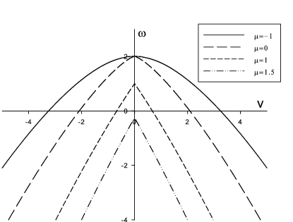
Figure 2: Boundaries of the existence regions for soliton in $(v,\omega)$ plane for different $\mu$. Allowable values of $v$ and $\omega$ lie below the boundaries.

Equations (34) of the boundary of the soliton existence region coincide with the condition of the spin-wave instability. The existence regions for a few values of the parameter $\mu$ are shown in Fig.2. For $\mu<0$ the region has a form similar to the case $\lambda=0$ with the quadratic dependence $\omega_{0}(v)$ near the maximum point ($v=0,\ \omega=2$). For the case $\mu=0$ this dependence becomes $\omega_{0}=2-3v^{4/3}/4$. When $\mu>0$, the dependence $\omega_{0}(v)$ shifts down and a cusp appears at the maximal point ($v=0,\ \omega=2-\mu^{2}$).

The region of the soliton existence contains allowable values of $v$ and $\omega$ for a given $\mu$. As it can be seen in Fig.2 the soliton can exist in the spiral phase ($\mu>0.992$). But, for example, the kink is unstable for $\mu>\sqrt{2}$ since the point ($v=0,\ \omega=0$) corresponding to the kink does not belong to the existence region. It is worth noting that one should be careful in treating of the part of the existence region with large negative $\omega$, where the derivatives of $\theta(x)$ and $\varphi(x)$ near the center of soliton become large and the continuum approximations Eqs.(5), (16) become doubtful.

Within the existence region the roots of Eq.(33) have the forms

$$\kappa_{1,3} = \pm a_{1}+ib$$

$$\kappa_{2,4} = \pm a_{2}-ib$$ (35)

where $a_{1}$, $a_{2}$ and $b$ are real nonnegative quantities and $a_{1}\leq a_{2}$. Certainly, one should take into account only the roots providing the decay of $|\psi|$ at the corresponding limit. For determinacy we will consider the limit $(\xi-v\tau)\to\infty$ and, therefore, analyze the roots $\kappa_{1}=a_{1}+ib$ and $\kappa_{2}=a_{2}-ib$. At infinity only the root $\kappa_{1}$ with the smaller real part is vital. So, the asymptotes of the angles at $(\xi-v\tau)\to\infty$ are $\theta\sim\exp[-a_{1}(\xi-v\tau)]$ and $\varphi=-\omega\tau-b(\xi-v\tau)$.

The case of the static soliton ($v=0$) requires special treatment, because in this case both roots $\kappa_{1}$ and $\kappa_{2}$ have equal real parts $a_{1}=a_{2}$ (they immediately split if $v\neq 0$). Fortunately, for the static soliton the solution of Eq.(33) can be obtained explicitly and this allows to analyze in detail the behavior of the soliton asymptotes for given values of $\mu$ and $\omega$. The decaying roots at $(\xi-v\tau)\to\infty$ are

$$\kappa_{1}=\sqrt{-2\mu-2\sqrt{\mu^{2}-2+\omega}}$$ (36)

and $\kappa_{2}=\kappa_{1}^{*}$.

Simple analysis of Eq.(36) shows that there are three regimes of the asymptotic (31). The exponent $\kappa_{1}$ is real for $\mu<-\sqrt{2-\omega}$, which means that $\theta(\xi)$ smoothly tends to zero at infinity. This region lies totally in the ferromagnetic phase. In the region $-\sqrt{2-\omega}<\mu<\sqrt{2-\omega}$ the parameter $\kappa_{1}$ contains both real and imaginary parts. Here the superposition of asymptotes (31) with $\kappa_{1}$ and $\kappa_{2}=\kappa_{1}^{*}$ results in the decay with oscillation at infinity: $\theta(\xi)\sim e^{-a_{1}\xi}\sin(b\xi)$ and $\varphi=\rm{const}$. Finally, for $\mu>\sqrt{2-\omega}$ the parameter $\kappa_{1}$ is pure imaginary, which implies that the solution oscillates but does not decay at infinity. Therefore, in this region there are no static soliton-like excitations.

As was noted above only one asymptotic with $\kappa_{1}$ having smaller real part survives at infinity for $v\neq 0$. This implies that the asymptotic of the function $\theta(\xi)$ has no zeros. However, in the region close to the soliton center the function $\theta(\xi)$ can have a finite number of zeros and it is really observed numerically.

Generally, the relation between the parameters $\omega,v$ and $\nu,k$ is unknown analytically. However, it can be found for large values of $\nu$. For large solitons ($\nu\gg 1$) the soliton energy and, therefore, the scaling function $f(\mu,\nu,k)$ saturates to some finite value. This means that for $\nu\gg 1$ both $\omega\to 0$ and $v\to 0$. The boundaries between the regions corresponding to different asymptotic regimes for large solitons are obtained from the above analysis and they are shown in Fig.1. As one can see in Fig.1 the oscillating large solitons exist not only in the ferromagnetic phase but, partly, in the spiral phase region $0.992<\mu<\sqrt{2}$. The amplitude of the soliton oscillations grow as $\mu$ increases and the oscillations are most strong in the spiral phase. However, one should remember that the soliton excitations in the spiral phase lie in the high-energy part of the spectrum, because the energy of the soliton-like solutions differs from the ferromagnetic one on some finite value (26). Therefore, the soliton energy is higher than the spiral one (23) on the value proportional to the system size. Nevertheless, these states can be important in strong magnetic field close to the saturation value.

If we expand $n_{z}\approx 1-|\psi|^{2}/2$ and take into account the terms $\sim|\psi|^{2}\psi$ in Eq.(29), then Eq.(29) near the border of the soliton existence reduces to the modified non-linear Schrödinger equation containing the fourth-order derivative term

$$i\frac{\partial\psi}{\partial\tau}=\frac{1}{4}\frac{\partial^{4}\psi}{\partial\xi^{4}}+\mu\frac{\partial^{2}\psi}{\partial\xi^{2}}+2\psi-\frac{\omega+iv\kappa}{2}\left|\psi\right|^{2}\psi$$ (37)

Unfortunately, in spite of substantial simplification of the initial equation of motion (29), the exact solution of this equation is unknown and we have to use numerical calculation.

We note that Eqs.(31),(33) are valid for small $\alpha\ll 1$, but for any $\gamma$. In particular, for the case $\lambda=0$ ($\gamma=-1$) they correctly reproduce the known asymptotic for $\theta$ and $\varphi$.

IV Numerical calculations

We have carried out a numerical analysis of the discrete and the continuum versions of the classical spin model (2) in the vicinity of the IT point. Both energy functionals (4) and (18) were minimized numerically over angles $\theta_{n},\varphi_{n}$ and $\theta(x),\varphi(x)$ with fixed values of magnetization (8) and momentum (9). The periodic boundary conditions for soliton and the open boundary conditions for kink excitations were imposed. The numerical calculations showed that for small $\alpha$ the difference between the discrete and the continuum models is negligible as expected and it increases as $\alpha$ grows. On the investigation of the dynamics of solitons we restrict ourself to small anisotropy $\alpha\ll 1$, when the continuum approximation is valid, because in the discrete model with finite $\alpha$ a so-called pinning potential appears Mikeska ; IM and the momentum becomes undefined. So, on default we will present numerical results for the discrete classical model (4), keeping in mind that the continuum approach corresponds to the limit $\alpha\to 0$.

We studied the finite size effects for both discrete and continuum models and found that the system size $N$ should be taken so that the parameter $\alpha^{1/4}N\gg 1$. The finite size effects will be discussed in detail in Sec.V. Here we only notice that when the relation $\alpha^{1/4}N\gg 1$ is fulfilled the convergence of a solution accelerates exponentially with $N$.

At first we present and discuss the results for small values of $\alpha$ and $\gamma$, when the continuum approximation is justified and the soliton energy takes the scaling form (26). In order to verify the found scaling equation we plotted the results for a fixed $k$ and different values of $\alpha$, $\gamma$, $M$ as $E/(s^{2}\alpha^{3/4})$ vs. scaling parameters $\nu=\alpha^{1/4}M/s$ and $\mu=\gamma/\sqrt{\alpha}$. For small $\alpha$ and $\gamma$ all data must lie on one curve which actually represents the scaling function $f(\mu,\nu,k)$.

For example, the numerical data for the static solitons ($k=0$) and for $\mu=0$ is shown in Fig.3. Here the calculated dependencies of the soliton energy on the soliton size $M$ for three values of $\alpha=10^{-2}$, $10^{-3}$, $10^{-4}$ are demonstrated in axes $E/(s^{2}\alpha^{3/4})$ vs. $\nu=\alpha^{1/4}M/s$. As we see all three solid curves lie very close to each other and they rapidly converges in the limit $\alpha\to 0$, so that the curve corresponding to $\alpha=10^{-4}$ perfectly describes the scaling function $f(0,\nu,0)$.

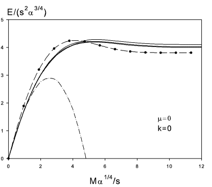
Figure 3: Scaled energy $E/s^{2}\alpha^{3/4}$ versus scaled soliton size $\nu=M\alpha^{1/4}/s$ for $\mu=0$ and $k=0$. Solid lines are soliton energies for three values of $\alpha=10^{-2},\ 10^{-3},\ 10^{-4}$ from top to bottom. Circles (joined by dashed line) are energies of magnon complexes of quantum $s=1/2$ F-AF chain for $N=24$ and $\alpha=0.05$ DK09 . Dot-dashed line is the energy of boson bound states of model (62).

The function $f(0,\nu,0)$, shown in Fig.3, reaches a maximum at $\nu\approx 5$ and then rapidly saturates, yielding the energy of large solitons $E\approx 4s^{2}\alpha^{3/4}$. For comparison we put also in Fig.3 similar data for $k=0$ and $\lambda=1/4$ obtained in Ref.DK09 for the quantum spin-$1/2$ chain of length $N=24$ and $\alpha=0.05$, which represents a rough estimate for the spin-$1/2$ scaling function $f_{1/2}(0,\nu,0)$. One can see that the behavior of the scaling functions for the quantum $s=1/2$ and the classical $s\to\infty$ models are very similar, though they have different limits at $\nu\to\infty$. Thus, we believe that the scaling law Eq.(26) is valid for quantum model (2) with general $s$ and the corresponding scaling functions $f_{s}$ behave similar to $f_{1/2}$ and $f$.

It is known Schneider that for $\lambda=0$ there is an equivalence between the energies of the classic static solitons of small size and the bound boson complexes of the Bose-Hamiltonian which is mapped from the anisotropic Heisenberg model. We expect that this mapping is valid for $\lambda\neq 0$ as well and it allows to determine the functional form of the energy for small solitons near the IT point. As it will be shown in Sec.VI the energy of the $M$-boson bound state of the corresponding Bose-model is

$$\frac{E}{s^{2}\alpha^{3/4}}=2\nu-\nu^{7/3}G_{b}(\beta)$$ (38)

where $\beta=\mu/\nu^{2/3}$ and the dependence $G_{b}(\beta)$ is shown in Fig.4.

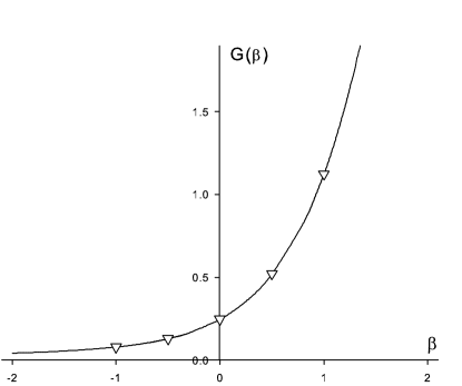
Figure 4: The functions $G(\beta)$ for the energy of small static solitons (triangles) and $G_{b}(\beta)$ for the energy of boson complexes Eq.(77) (solid line).

We found that the numerical data for $f(\mu,\nu,0)$ at $\nu\ll 1$ is perfectly fitted by Eq.(38) and the function $G(\beta)$ for the classical solitons perfectly coincides with $G_{b}(\beta)$ (see Fig.4). Therefore, we believe that the scaling functions for solitons and boson complexes are the same at $\nu\ll 1$ and are given by Eq.(38). However, they are different generally (see Fig.3). In particular, at $\nu\gg 1$ the energy of the soliton saturates while the boson complex energy diverges.

For small solitons with $k=0$ according to Eq.(32) $\omega$ is given by the derivative of the right-hand side of Eq.(38). Therefore, the boundary between different regimes of asymptotes given by equation $\mu^{2}=2-\omega$ (see Eq.(36)) transforms for small solitons to the relation $3\beta^{2}=7G-2\beta G^{\prime}$ for $\beta$. Numerical calculation of the function $G(\beta)$ (Fig.4) indicates that there is only one solution $\beta=-0.57$ of the above relation. This means that the oscillation behavior of the solitons of size $M$ exists if $\mu>-0.57\nu^{2/3}$ and that the first two terms in the expansion in small $\nu$ (38) is not sufficient to determine the boundary where solitons disappear.

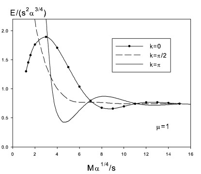
Figure 5: Scaled energy $E/s^{2}\alpha^{3/4}$ versus scaled soliton size $\nu=M\alpha^{1/4}/s$ for $\mu=1$ and for different $k$.

The scaling function $f(\mu,\nu,k)$ for $k=0,\ \pi/2,\ \pi$ at $\mu=1$ is demonstrated in Fig.5. As can be seen in Fig.5 the scaling function $f(1,\nu,k)$ converges at $\nu\to\infty$ to the same finite value for all $k$, which is natural, because the spectrum of large solitons is flat. Another observation followed from Fig.5 is that the scaling function for $\mu=1$ oscillates substantially stronger than that in the case $\mu=0$ (Fig.3).

As we have stated above the necessary condition for the soliton existence is

$$\frac{\partial f(\mu,\nu,k)}{\partial\nu}\leq\omega_{0}(\mu,v)$$ (39)

which means that $\partial f/\partial\nu\leq 2$ for $\mu\leq 0$ and $\partial f/\partial\nu\leq 2-\mu^{2}$ for $\mu\geq 0$ for any velocity.

This inequality imposes certain limitations on the soliton size (or the allowable values of $\nu$) with given values $\mu$ and $k$. However, the existence regions in the ($\nu,k$) plane can not be obtained directly from that in ($v,\omega$) plane, because the analytical relations between $\nu,\ k$ and $v,\ \omega$ near the IT point are unknown in contrast with the integrable case $\lambda=0$. Therefore, the stability of the soliton for different values of parameters $\mu$, $\nu$ and $k$ can be established by numerical minimization of the energy functional only. Our calculations show that for $\mu<0$ the solitons of any size and for all $k$ exist and inequality (39) is satisfied. However, the situation changes for $\mu>0$. For example, the solitons with $\mu=1$ and $k=0$ are stable for $\nu\gtrsim 1$ only as it is shown on Fig.5. As a matter of fact for $\mu>0$ only part of a whole phase space (a half-strip $\nu>0,\ 0<k<\pi$) is allowable for solitons. In general, the allowable region in ($\nu,k$) half-strip has a complicated form and can consist of many disconnected parts. For instance, at $\mu=1.5$ the static solitons with $k=0$ are stable in the range $3.5<\nu<8$ though for $k\neq 0$ small solitons exist.

Though a detailed phase picture can be find only numerically, nevertheless we can make some statements about it. Since soliton is a localized object, its energy inevitably saturates at $\nu\to\infty$ to some finite value independent of $k$. This means that for large solitons $\partial f/\partial\nu\to 0$. Therefore, for $\mu<\sqrt{2}$ all large enough solitons with $\nu>\nu_{\min}(\mu)$ are allowable. On the other hand deeply in the spiral phase when $\mu>\sqrt{2}$ the allowable region is restricted by $\nu<\nu_{\max}(\mu)$ and large solitons do not exist. In fact, we did not find large solitons for $\mu>\sqrt{2}$ in our calculations.

It is interesting to study the constraints on the soliton size in the isotropic limit of model (2) at $\lambda>1/4$, when $\alpha\to 0$ and $\mu\to\infty$. It can be shown that the function $f(\mu,\nu,k)$ at $\nu\ll 1$ and any $k\neq 0$ behaves as ($const/\nu^{3}$), where $const$ does not depend on $\alpha$. In this case condition (39) reduces to $\gamma M^{2}<const$. It means that the maximal possible size of soliton grows at $\gamma\to 0$. This fact qualitatively agrees with the observed behavior Kecke ; Laeuchli of the stability of magnon bound complexes with $k=\pi$ in the isotropic quantum $s=1/2$ F-AF model at $\lambda=1/4$. This is one more indication of the resemblance of the classical solitons and the quantum bound complexes in the F-AF model.

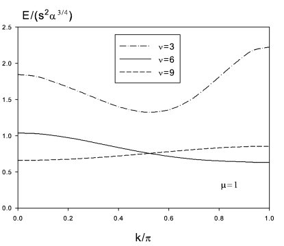
Figure 6: Energy momentum spectra at $\mu=1$ for $\nu=3$ (dot-dashed line), $\nu=6$ (dashed line) and $\nu=9$ (solid line).

In Fig.6 the dependence of the soliton energy on the momentum for $\mu=1$ is plotted for three different soliton sizes corresponding to $\nu=3$, $\nu=6$ and $\nu=9$. It is interesting to note that similarly to the case $\lambda=0$, there is a periodical dependence of the energy on the momentum in the continuum model near the IT point. We see that the dependence of the energy on the momentum rapidly flattens with the increase of the soliton size. In other words, the soliton mass exponentially grows with the soliton size. In this respect the behavior of the soliton spectrum is similar to the exactly solvable case $\lambda=0$ (see Eq.(10)). However, the dependence $E(k)$ has a very complex form in contrast to the case $\lambda=0$. As it is shown on Fig.6 $k_{\min}$ can be $k=0$, $k=\pi$ or even intermediate value between them. For $\nu=6$ the minimum of $E(k)$ is obtained at $k=\pi$. With the subsequent increase of the soliton size $\nu$ the form of the spectrum alternates: it has the minimum either at $k=0$ or at $k=\pi$. However, for $\nu>10$ the spectrum becomes so flat that it is difficult to distinguish these cases numerically. The soliton velocity $v$ is zero in both points $k=0$ and $k=\pi$.

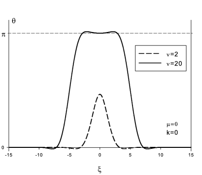
Figure 7: Shapes of small ($\nu=2$) and large ($\nu=20$) solitons for $\mu=0$ and $k=0$.

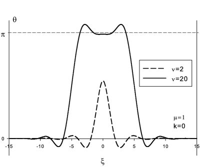
Figure 8: Shapes of small ($\nu=2$) and large ($\nu=20$) solitons for $\mu=1$ and $k=0$.

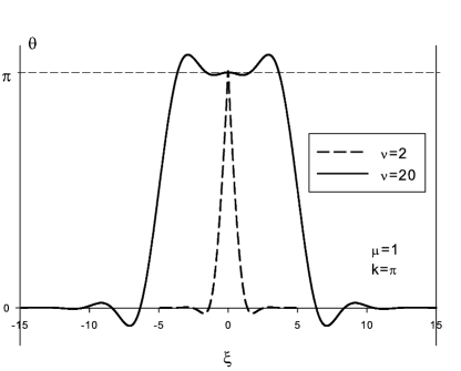
Figure 9: Shapes of small ($\nu=2$) and large ($\nu=20$) solitons for $\mu=1$ and $k=\pi$.

We have obtained numerically the soliton shapes for different values of the parameters $\mu$, $\nu$ and $k$. The shapes of static ($k=0$) solitons at $\mu=0$ for the cases $\nu=2$ and $\nu=20$ are demonstrated in Fig.7. The soliton solutions oscillate around $\theta=0$ (and $\theta=\pi$ for large soliton) and these oscillations exponentially decay as moving off the domain walls. Numerical calculations show that at approaching to the spiral phase the amplitude of the oscillations grows and its damping decreases with the distance from the soliton center. The shape of solitons of two different sizes with $\nu=2$ and $\nu=20$ at $\mu=1$, which is very close to the transition line, is shown in Fig.8. Here one can see the increase of oscillations in comparison with the case $\mu=0$. The observed behavior of the soliton shape is in full accord with conclusions followed from the analysis of Eq.(36).

The shape of solitons changes with the momentum $k$. This change is more pronounced for small solitons: they become narrower and higher. At the same time the shapes of large solitons remain almost the same. As an example the shapes of small and large solitons for the momentum $k=\pi$ and $\mu=1$ are demonstrated in Fig.9. As shown in Fig.9 the function $\theta(x)$ has a cusp at the maximum, which resembles the case $\lambda=0$. However, the behavior of the function $\varphi(\xi)$ drastically differs from the case $\lambda=0$ KosJETP . In particular, $\varphi(\xi)$ is discontinuous at $\xi=0$ in contrast with that for $\lambda=0$, where this function is linear near $\xi=0$.

One more illustration of the oscillation behavior of localized excitations in the F-AF model is the kink solution for the particular case $\mu=0$ ($\lambda=1/4$). Though we did not find the analytic solution of the non-linear equation (20), we found for this particular case some signs that it can admit a solution in a closed form. Namely, we studied numerically the kink excitation described by equation (20) with $\gamma=0$. The boundary conditions are $\theta(-\infty)=0$, $\theta(\infty)=\pi$ and $\theta^{\prime}(-\infty)=\theta^{\prime}(\infty)=0$. Numerical solution showed with very high accuracy that the asymptotic of the kink solution centered at $\xi=0$ has a form

$$\theta(\xi \to -\infty)=2\sin(1)\cos(-2^{1/4}\xi-1)e^{2^{1/4}\xi}$$

$$\theta(\xi \to \infty)=\pi-2\sin(1)\cos(2^{1/4}\xi-1)e^{-2^{1/4}\xi}$$ (40)

The oscillation behavior of the kink asymptotes is in full accord with Eq.(36).

At $|\xi|\ll 1$

$$\theta(\xi)=\frac{\pi}{2}+2^{1/4}\xi$$ (41)

Besides, the calculated kink energy has a surprisingly simple form

$$E=2s^{2}\alpha^{3/4}$$ (42)

where the numerical factor $2$ was found with high precision. Moreover, the contributions to this kink energy from different terms in Eq.(19) have simple rational ratios. All these facts together give a hope to obtain the exact solution of Eq.(20) for $\gamma=0$ in closed form.

The continuum approximation is valid for $\alpha\ll 1$. If the parameter $\alpha$ is not very small there are corrections to the soliton energy due to a discreteness. The energy of large soliton ($\nu\gg 1$) at $\lambda=1/4$ obtained numerically is shown in Fig.10. As one can see the energy is perfectly described by equation

$$E/s^{2}\approx 4\alpha^{3/4}+1.12\alpha^{5/4}$$ (43)

which is valid up to $\alpha\sim 1$. Here the first term is described by the continuum approximation, while the second term represents the correction coming from the discreteness of the lattice. The found correction to the soliton energy ($\sim\alpha^{5/4}$) differs from the correction to the energy of multimagnon complex ($\sim\alpha$) found for the case $s=1/2$ in Ref.DK09 .

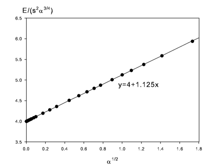
Figure 10: Dependence of the scaled energy of large solitons on the anisotropy $\sqrt{\alpha}$ for $\lambda=1/4$.

We found that similar behavior of the energy of the large soliton takes place for any $\mu$. So, the energy for $\nu\gg 1$ can be written as

$$E=s^{2}\alpha^{3/4}f(\mu)+s^{2}\alpha^{5/4}g(\mu)$$ (44)

where $f(\mu)$ is the saturated values of $f(\mu,\nu,k)$ at $\nu\to\infty$.

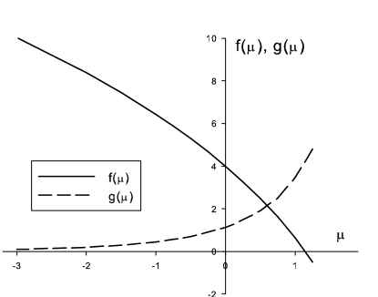
Figure 11: Functions $f(\mu)$ (solid line) and $g(\mu)$ (dashed line) describing two leading terms for the energy of large solitons (Eq.(44)).

The behaviors of the functions $f(\mu)$ and $g(\mu)$ are shown in Fig.11. As one can see $f(\mu)$ goes down with the increase of $\mu$ and becomes negative in the spiral phase at $\mu>1.2$. At the same time, the correction in Eq.(44) increases at approaching to the spiral phase.

In the opposed limit of large anisotropy $\alpha\gg 1$, the asymptotic of the soliton energy is found using a simple perturbation theory, which gives

$$E/s^{2}=4\alpha-8\lambda-\frac{2}{\alpha}-\frac{2\lambda^{2}}{\alpha s}+O(\alpha^{-2})$$ (45)

As follows from this equation the energy is not simply proportional to $s^{2}$ in contrast with the case $\lambda=0$ (Eq.(14)). This means that the dependence of the energy of kink or large soliton is not a universal function of $\alpha$ for general $s$ as it is for $\lambda=0$.

V Finite-size effects. Transition from uniform to localized solution.

In the preceding sections we investigated the soliton and the kink excitations of model (4) in the infinite system. Now we study the finite-size effects of these states. An interesting property of the soliton solutions of the classical model (4) on finite ring is the existence of the critical value $\alpha_{0}(L)$ below which the uniform solution ($\theta(x)=\mathrm{const}$) is realized. At $\alpha>\alpha_{0}$ this state develops into localized soliton. This transition from the uniform to the localized solution is similar to the well-known Gross-Pitaevskii transition in the Bose-systems BEGP .

We consider the static soliton on the ring of size $L$ with periodic boundary conditions. We use the continuous approach because the finite-size effects are essential at small values of $\alpha$. In the beginning we study the case $\lambda=0$. In this case the function $\theta(x)$ providing the extremum of the energy functional (7) satisfies the Lagrange-Euler equation

$$\frac{\partial^{2}\theta}{\partial x^{2}}=\alpha\sin(2\theta)-\alpha\omega\sin\theta,\qquad-\frac{L}{2}<x<\frac{L}{2}$$ (46)

with boundary conditions

$$\theta^{\prime}(0)=\theta^{\prime}(\pm L/2)=0$$ (47)

The Lagrange multiplier $\omega$ ensures the condition of a given normalized magnetization

$$n_{z}=\int\limits_{-L/2}^{L/2}\cos\theta\frac{\mathrm{d}x}{L}$$ (48)

Simple analysis shows that for any given values of $n_{z}$ and $L$ there is a critical value of parameter $\alpha=\alpha_{0}(n_{z},L)$ so that at $\alpha<\alpha_{0}$ Eq.(46) has a single and uniform solution $\theta(x)=\theta_{0}=\arccos(n_{z})$. The energy of this solution is

$$E=Ls^{2}\alpha(1-n_{z}^{2})$$ (49)

At $\alpha>\alpha_{0}$ another, non-trivial solution of Eq.(46) appears, which is a precursor of localized soliton solution. In particular, for the case $n_{z}=0$ the critical value is $\alpha_{0}=2\pi^{2}/L^{2}$ and the uniform solution at $\alpha<\alpha_{0}$ is $\theta_{0}=\pi/2$. The non-trivial solution at $\alpha\gtrsim\alpha_{0}$ can be expanded in small parameter $\vartheta=\sqrt{(\alpha-\alpha_{0})/2\alpha_{0}}\ll 1$:

$$\theta(\xi)=\pi/2+2\vartheta\cos\xi+2\vartheta^{3}\xi\sin\xi-\frac{\vartheta^{3}}{6}\cos(3\xi)$$ (50)

where $\xi=(2\alpha)^{1/2}x$.

The energy for this case can be written as

$$\frac{E}{s^{2}\sqrt{\alpha}} = l,\qquad l<l_{0}$$ (51)

$$\frac{E}{s^{2}\sqrt{\alpha}} = l-\frac{\sqrt{2}(l-l_{0})^{2}}{\pi},\qquad l\gtrsim l_{0}$$ (52)

where $l=L\sqrt{\alpha}$ and $l_{0}=\pi\sqrt{2}$. Therefore, the second derivative of $E$ with respect to $l$ is discontinuous at $l=l_{0}$ ($\alpha=\alpha_{0}$).

At $l\to\infty$ the solution for the case $n_{z}=0$ becomes

$$\tan\left(\theta/2\right)=\exp\left[\sqrt{2\alpha}(x+L/4)\right]$$ (53)

and $E$ tends to the known results $4s^{2}\sqrt{2\alpha}$.

A similar behavior of the soliton solution takes place for other values of $\lambda$. It is straightforward to obtain the value $\alpha_{0}$ and the soliton solution near $\alpha_{0}$ for the general case in the same manner as for the case $\lambda=0$. For example, for $\lambda=1/4$ and $n_{z}=0$ the critical value is $\alpha_{0}=2\pi^{4}/L^{4}$ and the solution at $\alpha\gtrsim\alpha_{0}$ is

$$\theta(\xi)=\frac{\pi}{2}+\vartheta\cos\xi+\frac{\vartheta^{3}}{2}\xi\sin\xi+\frac{\vartheta^{3}}{60}\cos(3\xi)$$ (54)

where $\xi=(8\alpha)^{1/4}x$.

The energy in this case is

$$\frac{E}{s^{2}\alpha^{3/4}} = l,\qquad l<l_{0}$$

$$\frac{E}{s^{2}\alpha^{3/4}} = l-\frac{3(l-l_{0})^{2}}{2^{1/4}\pi},\qquad l\gtrsim l_{0}$$ (55)

where $l=\alpha^{1/4}L$ and $l_{0}=2^{1/4}\pi$.

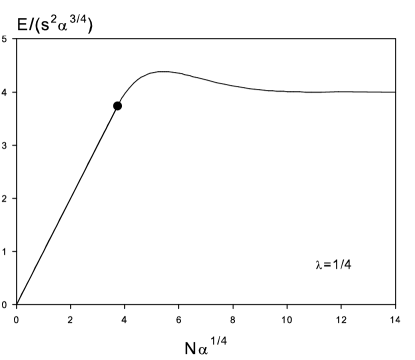
Figure 12: Scaled soliton energy versus finite-size parameter $N\alpha^{1/4}$ for $\lambda=1/4$ and $k=0$. Circle is a critical point of soliton creation.

The calculated dependence $E(l)$ for $\lambda=1/4$ and $n_{z}=0$ is shown in Fig.12. As one can see the energy rapidly saturates to its asymptotic value at $l>l_{0}$. Therefore, in order to reduce finite-size effects in numerical calculations near the transition point $\lambda=1/4$ one should choose the system size $N$ so that the parameter $\alpha^{1/4}N>10$.

The critical $\alpha_{0}$ for a given magnetization $n_{z}$ can be restored from the case $n_{z}=0$ by the relation

$$\alpha_{0}(n_{z},L)=\frac{\alpha_{0}(0,L)}{1-n_{z}^{2}}$$ (56)

The process of the formation of the kink (domain-wall) occurs in a somewhat different way. The kink is realized in open chain with the boundary conditions $\theta(-L/2)=0$, $\theta(L/2)=\pi$. In this case the lowest state at small $\alpha$ is the spiral one

$$\theta(x)=\frac{\pi}{2}+\frac{\pi x}{L}$$ (57)

and its energy remains finite at $\alpha=0$ in contrast with the solitons. For example, for $\lambda=1/4$ it is

$$E=s^{2}\frac{2\pi^{4}}{L^{3}}+s^{2}\frac{\alpha L}{2}$$ (58)

When $\alpha$ increases the spiral configuration continuously transforms to the kink. In this respect the situation is different from the definite and sharp transition from the uniform to soliton-like state studied before. The crossover between the spiral and the kink states takes place at $l\sim 1$. At $l\to\infty$ the energy of the kink is a half energy of the soliton.

It is worth noting that the transition of such kind coming from the finite-size effects occurs in the quantum spin model (2) as well. For very small $\alpha$, when the corresponding parameter $l\ll 1$, the system is in a uniform state, which is the state with a given total projection $S^{z}$ and the maximal total spin $S=S_{\max}=sN$. The energy of this state is given by Eq.(49) with $n_{z}=S^{z}/sN$ as in the classical model. This uniform state transforms continuously to the localized state of bound magnon complex when $\alpha$ increases. The crossover between the uniform and the localized states takes place at $\alpha^{1/2}N\sim 1$ for $\lambda=0$ and at $\alpha^{1/4}N\sim 1$ for $\lambda=1/4$.

VI Quantum model. Mapping to $\delta$-attractive bose model.

It is known that there is a resemblance between the classical solitons and the quantum magnon complexes at $\lambda=0$ Schneider . In the preceding sections we observed such a resemblance for the classical F-AF model and its quantum counterpart with $s=1/2$ as well. Here we consider the excitations in the quantum model with general $s$ and compare them with the classical solitons. A standard method to treat the quantum spin models is a mapping of the spin-Hamiltonian to the Bose-one. Though this method is approximate it gives important indications about the behavior of the spin systems. Using the Dyson-Maleev transformation

$$S_{i}^{z} = a_{i}^{+}a_{i}-s$$

$$S_{i}^{+} = \sqrt{2s}a_{i}^{+}\left(1-\frac{a_{i}^{+}a_{i}}{2s}\right)$$

$$S_{i}^{-} = \sqrt{2s}a_{i}$$ (59)

we represent the Hamiltonian (2) in the form

$$H=\sum_{k}\varepsilon_{k}a_{k}^{+}a_{k}+\frac{1}{N}\sum_{k_{1},k_{2},q}V(k_{1},k_{2},q)a_{q+k_{1}}^{+}a_{q-k_{1}}^{+}a_{q+k_{2}}a_{q-k_{2}}$$ (60)

where $a_{k}$ and $a_{k}^{+}$ are conventional bose-operators.

In the long-wavelength and weakly-coupling limit $V(k_{1},k_{2},q)=-\alpha$ and the one-magnon spectrum $\varepsilon_{k}$ in the vicinity of the IT point is

$$\varepsilon_{k}=2s\alpha-s\gamma k^{2}+\frac{sk^{4}}{4}$$ (61)

In this limit Hamiltonian (60) is equivalent to the Bose-model with the attractive $\delta$ -function interaction

$$H=2sm\alpha+s\sum_{i=1}^{m}\left(\gamma\frac{\partial^{2}}{\partial x_{i}^{2}}+\frac{1}{4}\frac{\partial^{4}}{\partial x_{i}^{4}}\right)-2\alpha\sum_{j>i=1}^{m}\delta(x_{i}-x_{j})$$ (62)

where $m$ denotes number of the Bose particles. For the case $\lambda=0$ one can neglect the fourth-order derivative term and such model becomes exactly solvable one Guire . However, in the vicinity of the IT point the fourth-order derivative term in Eq.(62) is important and it destroys the exact solution found in Ref.Guire . Therefore, we have to use approximations.

First, we consider the two-boson bound state near the IT point and compare it with the two-magnon bound state found in Ref.DK09 . The wave function of two bosons with the total momentum $2k$ and the energy $E_{2}$ is $\Psi(x_{1},x_{2})=e^{ik(x_{2}+x_{1})}\psi(x_{2}-x_{1})$. The function $\psi$ is determined from the Schrödinger equation

$$(2s\gamma-3sk^{2})\frac{\partial^{2}\psi(x)}{\partial x^{2}}+\frac{s}{2}\frac{\partial^{4}\psi(x)}{\partial x^{4}}-2\alpha\delta(x)\psi(x)=\varepsilon_{b}\psi(x)$$ (63)

where $x=x_{2}-x_{1}$ and $\varepsilon_{b}=2\varepsilon_{k}-E_{2}$ ($\varepsilon_{b}>0$) is the binding energy. Here we see that the fourth-order derivative term introduces the dependence of the function $\psi(x)$ and the binding energy $\varepsilon_{b}$ on the total momentum.

The function $\psi(x)$ as well as its first- and second-order derivatives are continuous at $x=0$, while the third-order derivative satisfies the condition

$$\frac{s}{4}\left.\frac{\partial^{3}\psi}{\partial x^{3}}\right|_{-0}^{+0}=\alpha\psi(0)$$ (64)

The wave function of the bound state of two particles with $\delta$ -attraction has a form:

$$\psi(x)=e^{-\kappa|x|}\left[\eta\cos(\eta x)+\kappa\sin(\eta|x|)\right]$$ (65)

where the parameters $\kappa$ and $\eta$ are determined by the above stated conditions for the function $\psi(x)$ and its derivatives at $x=0$. The solution has a form

$$\kappa = \left(\frac{\alpha}{4s}\right)^{1/3}g(\beta)$$

$$\eta = \left(\frac{\alpha}{4s}\right)^{1/3}\sqrt{8\beta+g^{2}(\beta)}$$ (66)

where

$$\beta = \frac{\gamma-3k^{2}/2}{\left(2\alpha/s\right)^{2/3}}$$ (67)

$$g(\beta) = \left(1+\sqrt{1+(4\beta/3)^{3}}\right)^{1/3}-\frac{4\beta/3}{\left(1+\sqrt{1+(4\beta/3)^{3}}\right)^{1/3}}$$ (68)

The binding energy is

$$\varepsilon_{b}=\frac{2^{1/3}\alpha^{4/3}}{s^{1/3}g^{2}(\beta)}$$ (69)

In particular, for $\gamma=0$ ($\lambda=1/4$) and $k=0$ it is

$$\varepsilon_{b}=\frac{\alpha^{4/3}}{(2s)^{1/3}}$$ (70)

The wave function (65) has one interesting feature. It oscillates when $\eta$ is real and has a form of superposition of two decaying exponents otherwise: $\psi(x)=e^{-\kappa_{1}|x|}+ce^{-\kappa_{2}|x|}$. The boundary between these regions is defined by equation $\eta=0$, which has a solution $\beta=-1/2^{5/3}$. Thus, the wave function of two coupled bosons oscillates for $2\gamma>3k^{2}-(\alpha/s)^{2/3}$ and does not oscillate for $2\gamma\leq 3k^{2}-(\alpha/s)^{2/3}$. The oscillation region diminishes with the increase of the total momentum. Certainly, the oscillatory behavior of the wave function is the effect of the frustration similarly to that observed for the solitons in the spin model.

We can compare Eq.(70) with the binding energy of two magnons for $s=1/2$ found by us in DK09

$$E_{b}=\alpha^{4/3}-\frac{2}{3}\alpha^{5/3}+O(\alpha^{2})$$ (71)

It follows from Eqs.(70) and (71) that the leading term in $E_{b}$ at $\alpha\to 0$ coincides up to numerical factor with the two-boson binding energy, but subsequent terms in the expansion of $E_{b}$ are absent in (70). Similar difference between $E_{b}$ and $\varepsilon$ takes place for any values of $\lambda$. For example, for $\lambda=0$ it is

$$\varepsilon_{b} = \frac{\alpha^{2}}{2s}$$

$$E_{b} = \frac{\alpha^{2}}{2s}-\frac{4s-1}{8s^{3}}\alpha^{3}+O(\alpha^{4})$$ (72)

As will be shown below, this difference plays a key role at comparison of the multimagnon and multiboson bound states.

The exact wave function of the $m$-boson state at $\lambda=0$ is known for any $m$ Guire . As was shown in Ref.Calogero at $\lambda=0$ the Hartree approximation correctly reproduces the exact energy of the multiboson states ($m\gg 1$) with zero total momentum. Therefore, we expect that this approach gives reliable results for $m\gg 1$ when $\lambda\neq 0$. Here we consider Bose model (62) in a parametric regime corresponding to the vicinity of the IT point of model (2).

The energy functional for zero total momentum in the Hartree approximation is

$$E_{m}=2sm\alpha+m\int_{-\infty}^{\infty}\mathrm{d}x\left[-s\gamma\left(\frac{\partial\phi}{\partial x}\right)^{2}+\frac{s}{4}\left(\frac{\partial^{2}\phi}{\partial x^{2}}\right)^{2}-m\alpha\phi^{4}\right]$$ (73)

Rescaling $\xi=(m\alpha/s)^{1/3}x$ and $\phi(\xi)=(m\alpha/s)^{1/6}\chi(\xi)$ transforms the energy functional (73) to

$$E_{m}=2sm\alpha+sm(\frac{m\alpha}{s})^{4/3}\int_{-\infty}^{\infty}\mathrm{d}\xi\left[-\beta\left(\frac{\partial\chi}{\partial\xi}\right)^{2}+\frac{1}{4}\left(\frac{\partial^{2}\chi}{\partial\xi^{2}}\right)^{2}-\chi^{4}(\xi)\right]$$ (74)

where $\beta=\gamma/(m\alpha/s)^{2/3}$. The function $\phi(x)$ satisfies the conventional normalization condition, which after rescaling gives the same normalization condition for $\chi(\xi)$

$$\int_{-\infty}^{\infty}\phi^{2}(x)\mathrm{d}x=\int_{-\infty}^{\infty}\chi^{2}(\xi)\mathrm{d}\xi=1$$ (75)

The Hartree equation comes from the minimization of the energy over $\chi(\xi)$. For $m\gg 1$ it has a form:

$$\beta\frac{\partial^{2}\chi}{\partial\xi^{2}}+\frac{1}{4}\frac{\partial^{4}\chi}{\partial\xi^{4}}-2\chi^{3}=\epsilon\chi$$ (76)

where $\epsilon$ is the Lagrange multiplier secured the norma condition (75).

Unfortunately, the solution of this equation at present is unknown. However, if we assume the existence of a localized solution of Eq.(76), then the integral in Eq.(74) converges yielding some function of parameter $\beta$. So, the energy of $m$-boson bound complex takes the form

$$E_{m}=2sm\alpha-sm(\frac{m\alpha}{s})^{4/3}G_{b}(\beta)$$ (77)

The behavior of the function $G_{b}(\beta)$ obtained by the numerical minimization of the functional (74) is demonstrated in Fig.4. Numerical calculations also showed that there is a critical value of the parameter $\beta\approx-0.57$ separating the regions with ($\beta>-0.57$) and without ($\beta<-0.57$) oscillations of the function $\phi(x)$. The value $\beta=-0.57$ is the same as was found for the classical spin model, which certificates the distinct correspondence between the boson and the classical spin models for small solitons. However, the bound complex of bosons exists in the whole region of parameter $\beta$, which means that the instability of solitons studied in Sec.III comes from the effects neglecting in the boson approach.

It is interesting to compare Eq.(77) with the energy of the $m$-magnon bound state of the quantum model (2) with $s=1/2$ at $\lambda=1/4$. The latter has been obtained in Ref.DK09 and has a form

$$E_{m}=m\alpha-C_{1}m^{7/3}\alpha^{4/3}+C_{2}m^{11/3}\alpha^{5/3}+\ldots$$ (78)

where $C_{1}$ and $C_{2}$ are numerical coefficients.

Similarly to the case $m=2$ the leading terms of the expansions of these two energies in small $\alpha$ coincide with Eq.(77) up to numerical factors. However, energy (77) tends to $-\infty$ at $m\to\infty$ (collapse phenomenon), while the energy of $m$-magnon bound complex in the spin model are finite at $m\to\infty$ and behaves as $E_{m}\sim\alpha^{3/4}$ DK09 . Therefore, subsequent terms in the energy expansion in $\alpha$ of the spin model are responsible for a short distance repulsion of magnons preventing the collapse.

A comparison of the expression for the energy of the classical soliton of size $M$ (26) with a formula for the energy of $m$-boson complex (77) indicates that the obtained expression for the energy of $m$-boson complex (77) is a particular case of a more general scaling relation (26) for $k=0$ and

$$f_{b}(\mu,\nu,0)=2\nu-\nu^{7/3}G_{b}\left(\frac{\mu}{\nu^{2/3}}\right)$$ (79)

As we discussed in Sec.IV the scaling function of the boson model $f_{b}(\mu,\nu,0)$ at $\nu\ll 1$ coincides with the scaling function of the classical spin model. The comparison of this equation with Eq.(26) allows us to assume that Eq.(79) represents two first terms of the scaling function of the quantum spin-$s$ model (including the classical limit) in small parameter $\nu$

$$f_{s}(\mu,\nu,0)=\sum_{n=0}^{\infty}\nu^{4n/3+1}g_{n,s}\left(\frac{\mu}{\nu^{2/3}}\right)$$ (80)

where functions $g_{n,s}$ depend on $s$.

Eq.(79) reproduces (probably exactly for any $s$) two first terms in this expansion. But the expansion (80) contains infinite number of terms in contrast with Eq.(79). It leads to the finite energy of both the classic solitons and the quantum bound magnon complexes while the energy of $m$-boson complex diverges at $m\to\infty$.

Summarizing all the above facts, we believe that the bound energy of $m$ -magnon complex for a quantum spin-$s$ model (2) near the IT point is correctly described by the classical scaling formula (26)

$$E=s^{2}\alpha^{3/4}f_{s}(\mu,\nu,k)$$ (81)

The scaling functions $f_{s}$ for quantum spin-$s$ case does not coincide with the function $f$ obtained in the classical continuum approach, though all of them have very similar behavior and $\lim\limits_{s\to\infty}f_{s}=f$.

VII Conclusion

We studied the soliton excitations in the classical F-AF model with the easy-axis anisotropy. The F-AF model has two parameters: the frustration parameter $\lambda=|J_{2}|/J_{1}$ and the anisotropy $\alpha$. We found that in a weakly anisotropic limit ($\alpha\ll 1$) the behavior of the soliton solutions for small frustration parameter $\lambda<1/4$ is qualitatively similar to that for the exactly solvable easy-axis XXZ chain ($\lambda=0$ case). However, the situation drastically changes near the IT point ($\alpha=0$, $\lambda=1/4$), where the transition from the ferromagnetic to the spiral ground state takes place in the isotropic case. In the vicinity of the IT point the corresponding energy functional in the continuum approximation qualitatively changes and does not admit the exact solution. The analysis of the derived energy functional allowed us to estimate the behavior of the transition line between the ferromagnetic to the spiral ground state in ($\alpha,\lambda$) plane near the IT point.

We mainly interested in the behavior of the solitons in the vicinity of the IT point. We showed that these localized states are separated from the ferromagnetic state by a finite gap. The dependence of the soliton energy (the gap) on model parameters near the IT point was established on a base of the scaling arguments. As a result we found that the soliton energy is proportional to $\sim\alpha^{3/4}$ and is expressed by the scaling function (26) depending on three scaling parameters: $\mu=(\lambda-1/4)/\sqrt{\alpha}$, the scaled soliton size $\nu$ and the momentum $k$.

The analysis of the asymptotic solutions of the corresponding equation of motion provided us with the necessary conditions of the soliton stability. It was shown that solitons of all sizes and any momentum exist when $\mu\leq 0$, while in the region $\mu>0$ there are definite restrictions on the soliton size $\nu$ and the momentum $k$. The distribution of the allowable values of the soliton parameters in ($\nu,k$) plane for $\mu>0$ has very complicated form, which can be determined numerically only. For example, the static solitons ($k=0$) only of the middle size $3.5<\nu<8$ are stable at $\mu=1.5$. Nevertheless, some facts about the soliton existence region was ascertained analytically and then confirmed by numerical calculations. In particular, small static ($k=0$) solitons are unstable for $\mu>0$, while small solitons with non-zero momentum exist for any $\mu$. Large solitons ($\nu\gg 1$) exist for $\mu<\sqrt{2}$ and, therefore, they survive in the part of the spiral phase $1\lesssim\mu<\sqrt{2}$. Though the soliton excitations in the spiral phase lie in the high-energy part of the spectrum, they can play an essential role in the magnetization processes.

In the isotropic limit ($\mu\to\infty$) only small solitons with non-zero momentum survive and the maximal allowable size of these solitons increases when the frustration parameter tends to the critical value $\lambda\to 1/4$. Such a dependence of the soliton size on the frustration parameter is qualitatively similar to the observation that the size of the multimagnon bound complexes with $k=\pi$ in the quantum F-AF model grows when $\lambda\to 1/4$.

We found that the frustration reveals itself in the oscillating shape of solitons. The amplitude of the oscillations grows at approaching to the spiral phase and further inside of it. Generally, at some value of $\mu$ the solution starts to oscillate without the decay at infinity, i.e., soliton-like solution with given values of $\nu$ and $k$ disappears.

We studied the finite-size effects on the soliton solutions. It was shown that the soliton solution on finite ring originates in the uniform (non-localized) state. The transition from the uniform to the soliton-like state occurs at the critical value of the anisotropy $\alpha_{0}(L)\sim L^{-4}$, below which the uniform solution is realized. This finite-size effect is similar to the well-known Gross-Pitaevskii transition in the Bose-systems.

In order to establish a connection between the properties of the solitons and the multi-magnon complexes of the quantum counterpart of this model we used the Dyson-Maleev mapping of the spin model to the Bose one. It turned out that the dependence of the energy of boson bound complexes on model parameters represents a particular case of the found scaling expression for the classical soliton energy. Moreover, the energy of the bound magnon complexes for quantum spin-$1/2$ model found by us before perfectly coincides with the scaling equation for soliton energy. Therefore, we believe that the bound energy of multi-magnon complex for a quantum spin-$s$ model near the IT point is characterized by the same critical exponents and by the identical scaling parameters as the soliton energy, though the corresponding scaling functions are different for different $s$. It is known that such a resemblance takes place for the Heisenberg ferromagnetic chain with an easy-axis anisotropy. Our study shows that the multi-magnon complexes behave substantially as the classical objects for the frustrated model as well.

For future it would be interesting to study the behavior of the classical spin model deeply in the spiral phase. We believe that it can help in understanding of unusual magnetization processes and shed light on the behavior of the multi-magnon complexes at high magnetic fields.

References

- (1) H.-J. Mikeska and A. K. Kolezhuk, in Quantum Magnetism, Lecture Notes in Physics Vol. 645, edited by U. Schollwöck, J. Richter, D. J. J. Farnell, and R. F. Bishop, Eds. (Springer-Verlag, Berlin, 2004), p. 1.
- (2) Y. Mizuno, T. Tohyama, S. Maekawa, T. Osafune, N. Motoyama, H. Eisaki, and S. Uchida, Phys. Rev. B 57, 5326 (1998).
- (3) T. Masuda, A. Zheludev, A. Bush, M. Markika, and A. Vasiliev, Phys. Rev. Lett. 92, 177201 (2004).
- (4) M. Hase, H. Kuroe, K. Ozawa, O. Suzuki, H. Kitazawa, G. Kido and T. Sekine, Phys. Rev. B 70, 104426 (2004).
- (5) S.-L. Drechsler, J. Malek, J. Richter, A. S. Moskvin, A. A. Gippius, and H. Rosner, Phys. Rev. Lett. 94, 039705 (2005).
- (6) L. Capogna, M. Mayr, P. Horsch, M. Raichle, R. K. Kremer, M. Sofin, A. Maljuk, M. Jansen, and B. Keimer, Phys. Rev. B 71, 140402 (2005).
- (7) J. Malek, S.-L. Drechsler, U. Nitzsche, H. Rosner, and H. Eschrig, Phys. Rev. B 78, 060508(R) (2008).
- (8) A. V. Chubukov, Phys. Rev. B 44, 4693 (1991).
- (9) C. Itoi and S. Qin, Phys. Rev. B 63, 224423 (2001).
- (10) V. Ya. Krivnov and A. A. Ovchinnikov, Phys. Rev. B 53, 6435 (1996).
- (11) D. V. Dmitriev and V. Ya. Krivnov, Phys. Rev. B 73, 024402 (2006).
- (12) F. Heidrich-Meisner, A. Honecker, and T. Vekua, Phys. Rev. B 74, 020403(R) (2006).
- (13) H. T. Lu, Y. J. Wang, S. Qin, and T. Xiang, Phys. Rev. B 74, 134425 (2006).
- (14) D. V. Dmitriev, V. Ya. Krivnov, and J. Richter, Phys. Rev. B 75, 014424 (2007).
- (15) L. Kecke, T. Momoi, and A. Furusaki, Phys. Rev. B 76, 060407(R) (2007); T. Hikihara, L. Kecke, T. Momoi, and A. Furusaki, Phys. Rev. B 78, 144404 (2008).
- (16) A. M. Laeuchli, J. Sudan, and A. Luscher, J. Phys. Conf. Series 145, 012057 (2009).
- (17) R. D. Somma and A. A. Aligia, Phys. Rev. B 64, 024410 (2001); R. Jafari and A. Langari, Phys. Rev. B 76, 014412 (2007); A. Avella, F. Mancini, and E. Plekhanov, Eur. Phys. J.: Cond. Matter, 66, 295 (2008).
- (18) D. V. Dmitriev and V. Ya. Krivnov, Phys. Rev. B 77, 024401 (2008).
- (19) D. V. Dmitriev and V. Ya. Krivnov, Phys. Rev. B 79, 054421 (2009).
- (20) J. D. Johnson and J. C. Bonner, Phys. Rev. B 22, 251 (1980).
- (21) T. Schneider, Phys. Rev. B 24, 5327 (1981).
- (22) H.-J. Mikeska and M. Steiner, Adv. Phys. 40, 191 (1991).
- (23) A. M. Kosevich, B. A. Ivanov and A. S. Kovalev, Phys. Rep. 194, 117 (1990).
- (24) M. Lakshmanan, Phys. Lett. A 61, 53 (1977); L. A. Takhtajan, Phys. Lett. A 64, 235 (1977).
- (25) A. A. Ovchinnikov, JETP Lett. 5, 38 (1967); I. G. Gochev, JETP 34, 892 (1972).
- (26) I. G. Gochev, JETP 58, 115 (1983).
- (27) B. A. Ivanov, A. Yu. Merkulov, V. A. Stephanovich, and C. E. Zaspel, Phys. Rev. B 74, 224422 (2006).
- (28) B. A. Ivanov and A. M. Kosevich, Sov. J. Low Temp. Phys. 9, 439 (1983).
- (29) C. Etrich, H.-J. Mikeska, E. Magyari, H. Thomas, and R. Weber, Z. Phys. B 62, 97 (1985).
- (30) B. A. Ivanov and H.-J. Mikeska, Phys. Rev. B 70, 174409 (2004).
- (31) A. M. Kosevich, B. A. Ivanov, and A. S. Kovalev, JETP Lett. 25, 486 (1977).
- (32) R. Kanamoto, H. Saito, and M. Ueda, Phys. Rev. A 67, 013608 (2003); G. M. Kavoulakis, Phys. Rev. A 67, 011601(R) (2003); K. Sakmann, A. I. Streltsov, O. E. Alon, and L. S. Cederbaum, Phys. Rev. A 72, 033613 (2003).
- (33) J. B. McGuire, J. Math. Phys. 5, 622 (1964).
- (34) F. Calogero and A. Degasperis, Phys. Rev. A 11, 265 (1975).