The Mass Structure of the Galaxy Cluster Cl0024+1654 from a Full Lensing Analysis of Joint Subaru and ACS/NIC3 Observations

Abstract

We derive an accurate mass distribution of the rich galaxy cluster Cl0024+1654 ($z=0.395$) based on deep Subaru $BR_{\rm c}z^{\prime}$ imaging and our recent comprehensive strong lensing analysis of HST/ACS/NIC3 observations. We obtain the weak lensing distortion and magnification of undiluted samples of red and blue background galaxies by carefully combining all color and positional information. Unlike previous work, the weak and strong lensing are in excellent agreement where the data overlap. The joint mass profile continuously steepens out to the virial radius with only a minor contribution $\sim 10\%$ in the mass from known subcluster at a projected distance of $\simeq 700\,$kpc$\,h^{-1}$. The cluster light profile closely resembles the mass profile, and our model-independent $M/L_{R}$ profile shows an overall flat behavior with a mean of $\langle M/L_{R}\rangle\simeq 230h(M/L_{R})_{\odot}$, but exhibits a mild declining trend with increasing radius at cluster outskirts, $r\lower 2.15277pt\hbox{$\;\buildrel>\over{\sim}\;$}0.6r_{\rm vir}$. The projected mass distribution for the entire cluster is well fitted with a single Navarro-Frenk-White model with a virial mass, $M_{\rm vir}=(1.2\pm 0.2)\times 10^{15}M_{\odot}\,h^{-1}$, and a concentration, $c_{\rm vir}=9.2^{+1.4}_{-1.2}$. This model fit is fully consistent with the depletion of the red background counts, providing independent confirmation. Careful examination and interpretation of X-ray and dynamical data, based on recent high-resolution cluster collision simulations, strongly suggest that this cluster system is in a post collision state, which we show is consistent with our well-defined mass profile for a major merger occurring along the line of sight, viewed approximately $2-3$ Gyr after impact when the gravitational potential has had time to relax in the center, before the gas has recovered and before the outskirts are fully virialized. Finally, our full lensing analysis provides a model-independent constraint of $M_{\rm 2D}(<r_{\rm vir})=(1.4\pm 0.3)\times 10^{15}M_{\odot}\,h^{-1}$ for the projected mass of the whole system, including any currently unbound material beyond the virial radius, which can constrain the sum of the two pre-merger cluster masses when designing simulations to explore this system.

1. Introduction

Cl0024+1654 ($z=0.395$) is the most distant cluster of galaxies discovered by Zwicky (1959), and is the focus of some of the most thorough studies of cluster properties, including the internal dynamical (Czoske et al., 2002; Diaferio et al., 2005), X-ray emission (Soucail et al., 2000; Ota et al., 2004; Zhang et al., 2005), and both weak (Kneib et al., 2003; Hoekstra, 2007; Jee et al., 2007) and strong (Colley et al., 1996; Tyson et al., 1998; Broadhurst et al., 2000; Comerford et al., 2006; Zitrin et al., 2009b) lensing work.

Despite the round and concentrated appearance of this cluster, several independent lines of evidence point to recent merging of a substantial substructure. The internal dynamics of about $300$ spectroscopically-measured galaxies has been modeled by a high-speed, line-of-sight collision of two systems with a mass ratio of the order of 2:1, leading to a compressed distribution of velocities along the line of sight (Czoske et al., 2001, 2002). A direct line-of-sight merger is also used to account for the “ring” of dark matter claimed by Jee et al. (2007), based on the central mass distribution derived from deep Hubble Space Telescope (HST) Advanced Camera for Surveys (ACS) images. On a larger scale, the mass distribution derived from a mosaic of HST/WFPC2 pointings (Kneib et al., 2003) reveals an additional substantial subcluster in the mass at a projected radius of $3\arcmin$ coincident with a noticeable concentration of galaxies. This substructure is however not along the line of sight, but is associated with the main cluster component in redshift space (Czoske et al., 2002), and lies $R\sim 700\,{\rm kpc}\,h^{-1}$ northwest (NW) in projection from the center of the main cluster.

No clear evidence of excess X-ray emission is found at the location of the NW galaxy clump, but interaction may be implied instead by the anomalously low level of X-ray emission relative to the standard X-ray luminosity–mass relation. The measured gas temperature is also unusually low, only $T_{X}\simeq 4.5$ keV (Ota et al., 2004), over the full range of radius ($R\lower 2.15277pt\hbox{$\;\buildrel<\over{\sim}\;$}300\,{\rm kpc}\,h^{-1}$) probed by deep Chandra data, whereas recent weak and strong lensing observations indicate that the cluster is a high-mass system with a total projected mass of $M_{\rm 2D}\lower 2.15277pt\hbox{$\;\buildrel>\over{\sim}\;$}10^{15}M_{\odot}$ (Hoekstra, 2007; Jee et al., 2007; Mahdavi et al., 2008; Zitrin et al., 2009b). The careful hydrodynamical simulations of Ricker & Sarazin (2001) predict that in a period of 1–3 Gyr (or a timescale of the sound crossing time, $\tau_{sc}$) after a substantial merger the hot gas associated with the whole system is extensively distributed so that the emissivity is actually markedly reduced by virtue of the lowered gas density, once the shock associated with the collision has dissipated. Furthermore, substantial proportion of the gas may escape from the system together with high velocity galaxies, so that the velocity dispersion of the remainder is significantly reduced. These lack of any observed hot shocked gas component implies very clearly that no merger has happened very recently, within a couple of Gyr, unlike the bullet cluster (Clowe et al., 2006) and other clusters caught in the first collisional encounter (Okabe & Umetsu, 2008).

Cl0024+1654 displays one of the finest examples of gravitational lensing forming a symmetric 5-image system of a well-resolved galaxy, which was first noted by Koo (1988) and later resolved into a close triplet of arcs by Kassiola et al. (1992), with two additional images found by Smail et al. (1996) and by Colley et al. (1996) using HST WFPC1 and WFPC2 data, respectively. These arcs have been used by Colley et al. (1996) to construct an image of the source, whose redshift $z=1.675$ (Broadhurst et al., 2000) permits an accurate and model-independent enclosed mass for the central $R<100\,{\rm kpc}\,h^{-1}$ area of $M(<R)=(1.11\pm 0.03)\times 10^{14}M_{\odot}\,h^{-1}$, with a central mass-to-light ratio of $(M/L)_{B}=(320\pm 30)h(M_{\odot}/L_{\odot})_{B}$ (Broadhurst et al., 2000).

More recently the central mass profile has been constrained by lensing with the identification of many new multiply lensed images (Zitrin et al., 2009b) in very deep multi-color imaging with HST/ACS as part of the ACS/GTO program (Ford et al., 2003). Here a joint fit was made to 33 lensed images and their photometric redshifts with a relatively simple 6-parameter description of the deflection field. This modeling method has been recently applied to two unique, X-ray luminous high-$z$ clusters, MACS J1149.5+2223 and MACS J0717.5+3745, uncovering many sets of multiply-lensed images (Zitrin & Broadhurst, 2009; Zitrin et al., 2009a). The high resolution and accuracy of colors allow a secure identification of counter images by delensing the pixels of candidate lensed images to form a source which is then relensed to predict the detailed appearance of counter images, a technique developed for similar high quality ACS/GTO data of A1689 (Broadhurst et al., 2005a). This model has been used to estimate the magnification of high-redshift candidate galaxies with photometric redshifts $z_{\rm phot}\sim 6-7$ identified in combining this data with deep near-infrared images (Zheng et al., 2009). Here we add to this new strong-lensing information with new weak-lensing data from deep, multi-color imaging with the Subaru telescope to examine the mass distribution in detail over the full profile of the cluster. These high-quality Subaru images span the full optical range in the $B$, $R_{\rm c}$, and $z^{\prime}$ passbands, allowing us to define a background sample of red and blue galaxies free from cluster member and foreground galaxies. We have learned from our earlier work that without adequate color information, the weak-lensing signal can be heavily diluted particularly towards the cluster center by the presence of unlensed cluster members (Broadhurst et al., 2005b; Medezinski et al., 2007; Umetsu & Broadhurst, 2008), so that weak lensing underpredicts the Einstein radius derived from strong-lensing studies and the gradient of the inner mass profiles based on weak lensing is also underestimated. Unfortunately, many examples of this problem are present in the literature, and here we carefully explore the weak-lensing signal in color-color space and by comparison with the deep photometric redshift survey in the COSMOS field (Ilbert et al., 2009).

A major motivation for pursuing improved lensing measurements is the increased precision of model predictions for the mass density profiles of cluster-size massive dark-matter halos based on $N$-body simulations in the standard $\Lambda$ cold dark-matter (hereafter $\Lambda$CDM) model (Hennawi et al., 2007; Neto et al., 2007; Duffy et al., 2008). Clusters of galaxies provide a definitive test of the standard structure-formation model because their mass density profiles, unlike galaxies, are not expected to be significantly affected by cooling of baryons (e.g., Blumenthal et al., 1986; Broadhurst & Barkana, 2008). This is because the high temperature and low density of the intra-cluster gas (hereafter ICG) prevents efficient cooling and hence the majority of baryons simply trace the gravitational potential of the dominant dark matter. Massive clusters are of particular interest in the context of this model, because they are predicted to have a distinctively shallow mass profile (or low concentration) described by the form proposed by Navarro et al. (1997) and this question has been the focus of our preceding work (Broadhurst et al., 2005b; Umetsu et al., 2007; Broadhurst et al., 2008; Umetsu & Broadhurst, 2008; Umetsu et al., 2009).

The paper is organized as follows. We briefly summarize in §2 the basis of cluster weak gravitational lensing. In §3 we describe the observations, the photometry procedure, the sample selection, and the weak-lensing shape analysis. In §4 we present our weak lensing methods, and derive the cluster lensing distortion and convergence profiles from Subaru weak lensing data. In §5 we examine in detail the cluster mass and light profiles based on the joint weak and strong lensing analysis. In §6 we compare our results with previous studies of Cl0024+1654 to examine the long-standing puzzle on large mass discrepancies between lensing and X-ray/dynamical methods, and investigate the implications of observed discrepancies and anomalies. In §7 we explore and discuss a possible interpretation of the observed X-ray features and mass discrepancies Finally, a summary is given in §8.

Throughout this paper, we use the AB magnitude system, and adopt a concordance $\Lambda$CDM cosmology with $\Omega_{m}=0.3$, $\Omega_{\Lambda}=0.7$, and $h\equiv H_{0}/(100\,{\rm km\,s^{-1}\,Mpc^{-1}})=0.7$. In this cosmology, $1\arcmin$ corresponds to $224$ kpc $h^{-1}$ (and $1\arcsec$ to $3.73$ kpc $h^{-1}$) at the cluster redshift. All quoted errors are 68.3% confidence limits unless otherwise stated. The reference sky position is the center of the central bright elliptical galaxy (the galaxy 374 in the spectroscopic catalog of Czoske et al. (2002)): ${\rm R.A.}=$ 00:26:35.69, ${\rm Decl.}=$ +17:09:43.12 (J2000.0). We refer to this position as the optical cluster center, hereafter. The cluster center of mass for our radial profile analysis is chosen to be the dark-matter center at $\Delta{\rm R.A.}=-2.32\arcsec$, $\Delta{\rm Decl.}=-1.44\arcsec$ of Zitrin et al. (2009b).

2. Basis of Cluster Weak Lensing

Weak gravitational lensing is responsible for the weak shape distortion and magnification of the images of background sources due to the gravitational field of intervening foreground clusters of galaxies and large scale structures in the universe (e.g., Umetsu et al., 1999; Bartelmann & Schneider, 2001). The deformation of the image can be described by the $2\times 2$ Jacobian matrix $\cal{A}_{\alpha\beta}$ ($\alpha,\beta=1,2$) of the lens mapping. The Jacobian ${\cal A}_{\alpha\beta}$ is real and symmetric, so that it can be decomposed as

$${\cal A}_{\alpha\beta} = (1-\kappa)\delta_{\alpha\beta}-\Gamma_{\alpha\beta},$$ (1)

$$\Gamma_{\alpha\beta} = \left(\begin{array}[]{cc}+{\gamma}_{1}&{\gamma}_{2}\\ {\gamma}_{2}&-{\gamma}_{1}\end{array}\right),$$ (4)

where $\delta_{\alpha\beta}$ is Kronecker’s delta, $\Gamma_{\alpha\beta}$ is the trace-free, symmetric shear matrix with $\gamma_{\alpha}$ being the components of spin-2 complex gravitational shear $\gamma:=\gamma_{1}+i\gamma_{2}$, describing the anisotropic shape distortion, and $\kappa$ is the lensing convergence responsible for the trace-part of the Jacobian matrix, describing the isotropic area distortion. In the weak lensing limit where $\kappa,|\gamma|\ll 1$, $\Gamma_{\alpha\beta}$ induces a quadrupole anisotropy of the background image, which can be observed from ellipticities of background galaxy images. The flux magnification due to gravitational lensing is given by the inverse Jacobian determinant,

$$\mu=\frac{1}{{\rm det}{\cal A}}=\frac{1}{(1-\kappa)^{2}-|\gamma|^{2}},$$ (5)

where we assume subcritical lensing, i.e., ${\rm det}{\cal A}(\mbox{\boldmath$\theta$})>0$.

The lensing convergence is expressed as a line-of-sight projection of the matter density contrast $\delta_{m}=(\rho_{m}-\bar{\rho})/\bar{\rho}$ out to the source plane ($s$) weighted by certain combination of co-moving angular diameter distances $r$ (e.g., Jain et al., 2000),

$$\kappa=\frac{3H_{0}^{2}\Omega_{m}}{2c^{2}}\int_{0}^{\chi_{s}}\!d\chi\,{\cal G}(\chi,\chi_{s})\frac{\delta_{m}}{a}\equiv\int\!d\Sigma_{m}\,\Sigma_{\rm crit}^{-1},$$ (6)

$${\cal G}(\chi,\chi_{s})=\frac{r(\chi)r(\chi_{s}-\chi)}{r(\chi_{s})},$$ (7)

where $a$ is the cosmic scale factor, $\chi$ is the co-moving distance, $\Sigma_{m}$ is the surface mass density of matter, $\Sigma_{m}=\int\!d\chi\,a(\rho_{m}-\bar{\rho})$, with respect to the cosmic mean density $\bar{\rho}$, and $\Sigma_{\rm crit}$ is the critical surface mass density for gravitational lensing,

$$\Sigma_{\rm crit}=\frac{c^{2}}{4\pi G}\frac{D_{s}}{D_{d}D_{ds}}$$ (8)

with $D_{s}$, $D_{d}$, and $D_{ds}$ being the (proper) angular diameter distances from the observer to the source, from the observer to the deflecting lens, and from the lens to the source, respectively. For a fixed background cosmology and a lens redshift $z_{d}$, $\Sigma_{\rm crit}$ is a function of background source redshift $z_{s}$. For a given mass distribution $\Sigma_{m}(\mbox{\boldmath$\theta$})$, the lensing signal is proportional to the angular diameter distance ratio,

$$\beta(z_{s})=\max\left[0,\frac{D_{ds}(z_{s})}{D_{s}(z_{s})}\right],$$ (9)

where $\beta(z_{s})$ is zero for unlensed objects with $z_{s}\leq z_{d}$.

In the present weak lensing study we aim to reconstruct the dimensionless surface mass density $\kappa(\mbox{\boldmath$\theta$})$ from weak lensing distortion data. For a two-dimensional mass reconstruction, we utilize the relation between the gradients of $\kappa$ and $\gamma$ (Kaiser, 1995; Crittenden et al., 2002),

$$\triangle\kappa(\mbox{\boldmath$\theta$})=\partial^{\alpha}\partial^{\beta}\Gamma_{\alpha\beta}(\mbox{\boldmath$\theta$})=2\hat{\cal D}^{*}\gamma(\mbox{\boldmath$\theta$})$$ (10)

where $\hat{\cal D}$ is the complex differential operator $\hat{\cal D}=(\partial_{1}^{2}-\partial_{2}^{2})/2+i\partial_{1}\partial_{2}$. The Green’s function for the two-dimensional Poisson equation is $\triangle^{-1}(\mbox{\boldmath$\theta$},\mbox{\boldmath$\theta$}^{\prime})=\ln|\mbox{\boldmath$\theta$}-\mbox{\boldmath$\theta$}^{\prime}|/(2\pi)$, so that equation (10) can be solved to yield the following non-local relation between $\kappa$ and $\gamma$ (Kaiser & Squires, 1993):

$$\kappa(\mbox{\boldmath$\theta$})=\frac{1}{\pi}\int\!d^{2}\theta^{\prime}\,D^{*}(\mbox{\boldmath$\theta$}-\mbox{\boldmath$\theta$}^{\prime})\gamma(\mbox{\boldmath$\theta$}^{\prime})$$ (11)

where $D(\mbox{\boldmath$\theta$})$ is the complex kernel defined as $D(\mbox{\boldmath$\theta$})=(\theta_{2}^{2}-\theta_{1}^{2}-2i\theta_{1}\theta_{2})/|\mbox{\boldmath$\theta$}|^{4}$. In general, the observable quantity is not the gravitational shear $\gamma$ but the complex reduced shear,

$$g=\frac{\gamma}{1-\kappa}$$ (12)

in the subcritical regime where ${\rm det}{\cal A}>0$ (or $1/g^{*}$ in the negative parity region with ${\rm det}{\cal A}<0$). We see that the reduced shear $g$ is invariant under the following global transformation:

$$\kappa(\mbox{\boldmath$\theta$})\to\lambda\kappa(\mbox{\boldmath$\theta$})+1-\lambda,\ \ \ \gamma(\mbox{\boldmath$\theta$})\to\lambda\gamma(\mbox{\boldmath$\theta$})$$ (13)

with an arbitrary scalar constant $\lambda\neq 0$ (Schneider & Seitz, 1995). This transformation is equivalent to scaling the Jacobian matrix ${\cal A}(\mbox{\boldmath$\theta$})$ with $\lambda$, $\cal{A}(\mbox{\boldmath$\theta$})\to\lambda{\cal A}(\mbox{\boldmath$\theta$})$. This mass-sheet degeneracy can be unambiguously broken by measuring the magnification effects, because the magnification $\mu$ transforms under the invariance transformation (13) as

$$\mu(\mbox{\boldmath$\theta$})\to\lambda^{2}\mu(\mbox{\boldmath$\theta$}).$$ (14)

3. Subaru Data and Analysis

In this section we present a technical description of our weak lensing analysis of Cl0024+1654 based on deep Subaru $BR_{\rm c}z^{\prime}$ images. The reader only interested in the main result may skip directly to §5.

3.1. Subaru Data and Photometry

For our weak-lensing analysis of Cl0024+1654 we retrieved from the Subaru archive, SMOKA, imaging data in $B$, $R_{\rm c}$, and $z^{\prime}$ taken with the wide-field camera Suprime-Cam ($34^{\prime}\times 27^{\prime}$; Miyazaki et al., 2002) at the prime-focus of the 8.3m Subaru telescope. The cluster was observed in the course of the PISCES program (Kodama et al., 2005; Umetsu et al., 2005; Tanaka et al., 2005). The FWHM in the co-added mosaic image is $1.27\arcsec$ in $B$, $0.80\arcsec$ in $R_{\rm c}$, and $0.82\arcsec$ in $z^{\prime}$ with $0.202\arcsec$ pixel^-1, covering a field of $\simeq 34\arcmin\times 26\arcmin$. The observation details of Cl0024+1654 are listed in Table 2. We use the $R_{\rm c}$-band data for our weak lensing shape measurements (described in §3.2) for which the instrumental response, sky background and seeing conspire to provide the best-quality images. The standard pipeline reduction software for Suprime-Cam (SDFRED, see Yagi et al., 2002; Ouchi et al., 2004) is used for flat-fielding, instrumental distortion correction, differential refraction, sky subtraction, and stacking. Photometric catalogs are constructed from stacked and matched images using SExtractor (Bertin & Arnouts, 1996). A composite $BR_{\rm c}z^{\prime}$ color image of the central $8\arcmin\times 8\arcmin$ region of the cluster is shown in Figure 1. Since our lensing work relies much on the colors of galaxies, special care has to be paid to the measurement of colors from $BR_{\rm c}z^{\prime}$ images with different seeing conditions. For an accurate measurement of colors the Colorpro (Coe et al., 2006) routine is used; this allows us to use SExtractor’s AUTO magnitudes for total magnitudes of galaxies and its isophotal magnitudes for estimation of colors, and applies a further correction for the different seeing between different bands. From the colors and magnitudes of galaxies we can safely select background galaxies (see §3.3) for the weak-lensing analysis.

Astrometric correction is done with the SCAMP tool (Bertin, 2006) using reference objects in the NOMAD catalog (Zacharias et al., 2004). Photometric zero-points were calculated from associated standard star observations taken on the same night. Since for $B$ and $R_{\rm c}$ only one standard field was taken, and for $z^{\prime}$-band only a few spectrophotometric standards are available, we further calculated zero-points by fitting galaxy templates to bright elliptical galaxies in this cluster, using BPZ (Benítez, 2000) in the Subaru three-band photometry combined with HST/ACS images taken in the $F435W,F625W$, and $F850LP$ bands, for which accurate zero-points are well known. Stars were also compared in both Subaru and the HST/ACS images. Finally, we find consistency of our magnitude zero-points to within $\pm 0.05$ mag.

3.2. Weak Lensing Distortion Analysis

We use the IMCAT package developed by N. Kaiser to perform object detection, photometry and shape measurements, following the formalism outlined in Kaiser et al. (1995, KSB). Our analysis pipeline is implemented based on the procedures described in Erben et al. (2001) and on verification tests with STEP1 and STEP2 data of mock ground-based observations (Heymans et al., 2006; Massey et al., 2007). For details of our implementation of the KSB+ method, see also Umetsu & Broadhurst (2008); Umetsu et al. (2009).

3.2.1 Object Detection

Objects are first detected as local peaks in the co-added mosaic image in $R_{\rm c}$ by using the IMCAT hierarchical peak-finding algorithm hfindpeaks which for each object yields object parameters such as a peak position, $x$, an estimate of the object size, $r_{g}$ (where $r_{g}$ is the Gaussian scale length of the object as given by hfindpeaks; see KSB for details), the significance of the peak detection, $\nu$. The local sky level and its gradient are measured around each object using the IMCAT getsky routine. Total fluxes and half-light radii, $r_{h}$, are then measured on sky-subtracted images using the IMCAT apphot routine. For details of our IMCAT-based photometry, see §4.2.1 of Umetsu et al. (2009). We removed from our detection catalog extremely small objects with $r_{g}<1$ pixel, objects with low detection significance, $\nu<10$, objects with large raw ellipticities, $|e|>0.5$ (see Clowe et al., 2000; Heymans et al., 2006; Massey et al., 2007) where $|e|=(a^{2}-b^{2})/(a^{2}+b^{2})$ with axis-ratio $0<b/a\leq 1$ for images with elliptical isophotes, noisy detections with unphysical negative fluxes, and objects containing more than $10$ bad pixels, ${\tt nbad}>10$. This selection procedure yields an object catalog with $N=82431$ ($93.2$ arcmin${}^{-}2$).

3.2.2 Weak Lensing Distortion Measurements

In the KSB algorithm we measure the complex image ellipticity $e_{\alpha}=\left\{Q_{11}-Q_{22},Q_{12}\right\}/(Q_{11}+Q_{22})$ from the weighted quadrupole moments of the surface brightness of individual galaxies,

$$Q_{\alpha\beta}=\int\!d^{2}\theta\,W({\theta})\theta_{\alpha}\theta_{\beta}I({\mbox{\boldmath$\theta$}})\ \ \ (\alpha,\beta=1,2)$$ (15)

where $I(\mbox{\boldmath$\theta$})$ is the surface brightness distribution of an object, and $W(\theta)$ is a Gaussian window function matched to the size of the object. In equation (15) the object centroid is chosen as the coordinate origin, and the maximum radius of integration is chosen to be $\theta_{\rm max}=4r_{g}$ from the centroid. In our practical implementation of equation (15), we iteratively refine the Gaussian-weighted centroid of each object to accurately measure the object shapes. An initial guess for the centroid is provided with the IMCAT hfindpeaks routine (see 3.2.1). During the process objects with offsets in each iteration larger than 3 pixels are removed (Oguri et al., 2009).

The next step is to correct observed image ellipticities for the point-spread function (PSF) anisotropy using a sample of stars as references:

$$e^{\prime}_{\alpha}=e_{\alpha}-P_{sm}^{\alpha\beta}q^{*}_{\beta}$$ (16)

where $P_{sm}$ is the smear polarizability tensor which is close to diagonal, and $q^{*}_{\alpha}=(P_{sm}^{*})^{-1}_{\alpha\beta}e_{*}^{\beta}$ is the stellar anisotropy kernel. We select bright ($20\lower 2.15277pt\hbox{$\;\buildrel<\over{\sim}\;$}R_{\rm c}\lower 2.15277pt\hbox{$\;\buildrel<\over{\sim}\;$}22$), unsaturated stellar objects identified in a branch of the $r_{h}$ versus $R_{\rm c}$ diagram to measure $q^{*}_{\alpha}$. In order to obtain a smooth map of $q^{*}_{\alpha}$ which is used in equation (16), we divided the co-added mosaic image of $\sim 10{\rm K}\times 7.7{\rm K}$ pixels into $4\times 3$ rectangular blocks, where the block length is based on the coherent scale of PSF anisotropy patterns (see, e.g., Umetsu & Broadhurst, 2008; Umetsu et al., 2009). In this way the PSF anisotropy in individual blocks can be well described by fairly low-order polynomials. We then fitted the $q^{*}$ in each block independently with second-order bi-polynomials, $q_{*}^{\alpha}(\mbox{\boldmath$\theta$})$, in conjunction with iterative outlier rejection on each component of the residual: $\delta e^{*}_{\alpha}=e^{*}_{\alpha}-(P_{sm}^{*})^{\alpha\beta}q^{*}_{\beta}(\mbox{\boldmath$\theta$})$. The final stellar sample contains 672 stars (i.e., $N_{*}\sim 60$ stars per block), or the mean surface number density of $n_{*}\simeq 0.75$ arcmin^-2, with $\nu\lower 2.15277pt\hbox{$\;\buildrel>\over{\sim}\;$}800$. We note that the mean stellar ellipticity before correction is $\bar{e_{1}}^{*}\simeq-3.5\times 10^{-3}$ and $\bar{e_{2}}^{*}\simeq-5.0\times 10^{-2}$ over the data field, while the residual $e^{*}_{\alpha}$ after correction is reduced to ${\bar{e}^{*{\rm res}}_{1}}=(-0.07\pm 1.18)\times 10^{-4}$ and ${\bar{e}^{*{\rm res}}_{2}}=(+2.10\pm 1.58)\times 10^{-4}$. The mean offset from the null expectation is reduced down to $|\bar{e}^{*\rm res}|=(2.1\pm 1.6)\times 10^{-4}$, which is almost two-orders of magnitude smaller than the weak lensing signal in cluster outskirts. We show in Figure 2 the quadrupole PSF anisotropy field as measured from stellar ellipticities before and after the anisotropic PSF correction. Figure 3 shows the distributions of stellar ellipticity components before and after the PSF anisotropy correction. From the rest of the object catalog, we select objects with $r_{h}>\overline{r_{h}^{*}}+\nu_{h}\sigma(r_{h}^{*})$ as a $R_{\rm c}$-selected weak lensing galaxy sample, where $\overline{r_{h}^{*}}$ is the median value of stellar half-light radii $r_{h}^{*}$, corresponding to half the median width of the circularized PSF over the data field, $\sigma(r_{h}^{*})$ is the rms dispersion of $r_{h}^{*}$, and $\nu_{h}$ is conservatively taken to be $1.5$ in the present weak lensing analysis.

We then need to correct image ellipticities for the isotropic smearing effect caused by atmospheric seeing and the window function used for the shape measurements. The pre-seeing reduced shear $g_{\alpha}$ ($\alpha=1,2$) can be estimated from

$$g_{\alpha}=(P_{g}^{-1})_{\alpha\beta}e^{\prime}_{\beta}$$ (17)

with the pre-seeing shear polarizability tensor $P^{g}_{\alpha\beta}$ defined as Hoekstra et al. (1998),

$$P^{g}_{\alpha\beta}=P^{sh}_{\alpha\beta}-\left[P^{sm}(P^{sm*})^{-1}P^{sh*}\right]_{\alpha\beta}\approx P^{sh}_{\alpha\beta}-P^{sm}_{\alpha\beta}\frac{{\rm tr}[P^{sh*}]}{{\rm tr}[P^{sm*}]}$$ (18)

with $P^{sh}$ being the shear polarizability tensor. In the second equality we have used a trace approximation to the stellar shape tensors, $P^{sh*}$ and $P^{sm*}$. To apply equation (17) the quantity ${\rm tr}[P^{sh*}]/{\rm tr}[P^{sm*}]$ must be known for each of the galaxies with different size scales. Following Hoekstra et al. (1998), we recompute the stellar shapes $P^{sh*}$ and $P^{sm*}$ in a range of filter scales $r_{g}$ spanning that of the galaxy sizes. At each filter scale $r_{g}$, the median $\langle{\rm tr}[P^{sh*}]/{\rm tr}[P^{sm*}]\rangle$ over the stellar sample is calculated, and used in equation (18) as an estimate of ${\rm tr}[P^{sh*}]/{\rm tr}[P^{sm*}]$. Further, we adopt a scalar correction scheme, namely

$$(P_{g})_{\alpha\beta}=\frac{1}{2}{\rm tr}[P_{g}]\delta_{\alpha\beta}\equiv P^{\rm s}_{g}\delta_{\alpha\beta}$$ (19)

(Erben et al., 2001; Hoekstra et al., 1998; Umetsu & Broadhurst, 2008; Umetsu et al., 2009).

Following the prescription in Umetsu & Broadhurst (2008) and Umetsu et al. (2009), we compute for each object the variance $\sigma_{g}^{2}$ of $g=g_{1}+ig_{2}$ from $N$ neighbors identified in the object size ($r_{g}$) and magnitude ($R_{\rm c}$) plane. We take $N=30$. The dispersion $\sigma_{g}$ is used as an rms error of the shear estimate for individual galaxies. With the dispersion $\sigma_{g}$ we define for each object the statistical weight $u_{g}$ by

$$u_{g}\equiv\frac{1}{\sigma_{g}^{2}+\alpha_{g}^{2}},$$ (20)

where $\alpha_{g}^{2}$ is the softening constant variance (e.g., Hamana et al., 2003). We choose $\alpha_{g}=0.4$, which is a typical value of the mean rms $\overline{\sigma}_{g}$ over the background sample (see, e.g., Umetsu & Broadhurst, 2008; Umetsu et al., 2009). The case with $\alpha_{g}=0$ corresponds to an inverse-variance weighting. On the other hand, the limit $\alpha_{g}\gg\sigma_{g}$ yields a uniform weighting. Figure 4 shows the mean statistical weight $\langle u_{g}\rangle$ as a function of object size $r_{g}$ (left) and of object magnitude $R_{\rm c}$ (right) for the $R_{\rm c}$-selected weak-lensing galaxy sample, where in each panel the mean weight is normalized to unity in the first bin.

3.2.3 Shear Calibration

In practical observations, the measurement of $P_{g}^{\rm s}$ is quite noisy for an individual faint galaxy. Further, $P_{g}^{\rm s}$ depends nonlinearly on galaxy shape moments (see, e.g., Bartelmann & Schneider (2001) for an explicit expression for the shape tensors), so that this nonlinear error propagation may lead to a systematic bias in weak lensing distortion measurements (T. Hamana, in private communication). Indeed, it has been found that smoothing noisy $P_{g}^{\rm s}$ estimates does not necessarily improve the shear estimate but can lead to a systematic underestimate of the distortion amplitude by $\sim 10\%$–$15\%$ (e.g., Erben et al., 2001; Heymans et al., 2006; Massey et al., 2007). In order to improve the precision in shear recovery, we have adopted the following shear calibration strategy: First, we select as a sample of shear calibrators those galaxies with a detection significance $\nu$ greater than a certain limit $\nu_{\rm c}$ and with a positive raw $P_{g}^{\rm s}$ value. Note that the shear calibrator sample is a subset of the target galaxy sample (see §3.2.1 and §3.2.2). Second, we divide the calibrator size ($r_{g}$) and magnitude ($R_{\rm c}$) plane into a grid of $10\times 3$ cells each containing approximately equal numbers of calibrators, and compute a median value of $P_{g}^{\rm s}$ at each cell in order to improve the signal-to-noise ratio. Finally, each object in the target sample is matched to the nearest point on the ($r_{g},R_{\rm c}$) calibration grid to obtain the filtered $P_{g}^{\rm s}$ measurement. In this study, we take $\nu_{\rm c}=30$ as the significance threshold for the calibrator sample. Finally, we use the estimator $g_{\alpha}=e^{\prime}_{\alpha}/\left<P_{g}^{\rm s}\right>$ for the reduced shear. The final $R_{\rm c}$-selected galaxy sample contains $N=38758$ objects, or the mean surface number density of $\bar{n}_{g}=43.7$ galaxies arcmin^-2. The mean variance over the galaxy sample is obtained as $\overline{\sigma_{g}^{2}}\simeq 0.20$, or $\overline{\sigma}_{g}\equiv(\overline{\sigma_{g}^{2}})^{1/2}\simeq 0.46$.

We have tested our weak lensing analysis pipeline including the galaxy selection procedure using simulated Subaru Suprime-Cam images of the STEP2 project (Massey et al., 2007). We find that we can recover the weak lensing signal with good precision: typically, $m\sim-5\%$ of the shear calibration bias, and $c\sim 10^{-3}$ of the residual shear offset which is about one-order of magnitude smaller than the weak-lensing signal in cluster outskirts ($|g|\sim 10^{-2}$). This level of calibration bias is subdominant compared to the statistical uncertainty ($\sim 15\%$) due to the intrinsic scatter in galaxy shapes, and the degree of bias depends on the quality of the PSF in a complex manner. Therefore, we do not apply shear calibration corrections to our data. Rather we emphasize that the most critical source of systematic uncertainty in cluster weak lensing is dilution of the distortion signal due to the inclusion of unlensed foreground and cluster member galaxies, which can lead to an underestimation of the true signal for $R\lower 2.15277pt\hbox{$\;\buildrel<\over{\sim}\;$}400\,$kpc$\,h^{-1}$ by a factor of $2-5$ (see Figure 1 of Broadhurst et al., 2005b).

3.3. Galaxy Sample Selection from the Color-Color Diagram

It is crucial in the weak lensing analysis to make a secure selection of background galaxies in order to minimize contamination by unlensed cluster and foreground galaxies; otherwise dilution of the distortion signal arises from the inclusion of unlensed galaxies, particularly at small radius where the cluster is relatively dense (Broadhurst et al., 2005b; Medezinski et al., 2007; Umetsu & Broadhurst, 2008). This dilution effect is simply to reduce the strength of the lensing signal when averaged over a local ensemble of galaxies, in proportion to the fraction of unlensed galaxies whose orientations are randomly distributed, thus diluting the lensing signal relative to the true background level, derived from the uncontaminated background level we will establish below.

To separate unlensed galaxies from the background and hence minimize the weak lensing dilution, we follow the background selection method recently developed by Medezinski et al. (2009), which relies on empirical correlations in color-color (CC) space derived from the deep Subaru photometry, by reference to the deep photometric redshift survey in the COSMOS field (see §3.4). For Cl0024+1654, we have a wide wavelength coverage ($BR_{\rm c}z^{\prime}$) of Subaru Suprime-Cam. When defining color samples, we require that objects are detected in all three Subaru bands. Further, we limit the data to $z^{\prime}\lower 2.15277pt\hbox{$\;\buildrel<\over{\sim}\;$}25.5$ AB mag in the reddest band available for the cluster. Beyond this limit incompleteness creeps into the bluer bands, complicating color measurements, in particular of red galaxies. Our CC-selection criteria yielded a total of $N=8676,1655$, and 5004 galaxies for the red, green, and blue samples, respectively, usable for our weak lensing distortion analysis; these correspond to mean surface number densities of $\bar{n}_{g}=10.9,2.1$, and 6.3 galaxies arcmin^-2, respectively. In Table 3, we list the magnitude limits, the total number of galaxies ($N$), the mean surface number density ($\bar{n}_{g}$), and the mean rms error for the galaxy shear estimate ($\overline{\sigma}_{g}$), for our color samples. The resulting color boundaries for respective galaxy samples are shown in Figure 5. We emphasize that this model-independent empirical method allows us to clearly distinguish these distinct blue and red populations (see Figures 5 and 6), by reference to the well-calibrated COSMOS photometry, as well as to separate unlensed foreground/cluster galaxies from the background (see also §3.4 and Figure 7).

3.3.1 Cluster Galaxies

Following the prescription by Medezinski et al. (2009) we construct a CC diagram and first identify in this space where the cluster lies by virtue of the concentration of cluster members. Figure 6 (left panel) shows in CC space the distribution of mean projected distances ($\theta$) from the cluster center for all galaxies in the Cl0024+1654 field. As demonstrated by Medezinski et al. (2009), this diagram clearly reveals the presence of strong clustering of galaxies with lower mean radius, confined in a distinct and relatively well-defined region of CC space. This small region corresponds to an overdensity of galaxies in CC space comprising the red sequence of the cluster and a blue trail of later type cluster members, as clearly demonstrated in the right panel of Figure 6. In Figures 5 (green points) and 6 (left panel) we mark this overdense region in CC space to safely encompass the region significantly dominated by the cluster. We term the above sample, which embraces all cluster member galaxies, the green sample, as distinct from well separated redder and bluer galaxies identified in this CC space (see the right panel of Figure 6). Naturally, a certain fraction of background galaxies must be also expected in this region of CC space, where the proportion of these galaxies can be estimated by comparing the strength of their weak lensing signal with that of the reference background samples (Medezinski et al., 2007, 2009). Figure 10 (crosses) demonstrates that the level of the tangential distortion for the green sample is consistent with zero to the outskirts of the cluster, indicating that the proportion of background galaxies in this sample is small compared with cluster members.

3.3.2 Red Background Galaxies

To define the foreground and background populations, we utilize the combination of the strength of the weak lensing signal and the number density distribution of galaxies in CC space. With the $BR_{\rm c}z^{\prime}$ photometry we can improve upon the simple color-magnitude selection previously performed in our weak lensing analyses of $z\sim 0.2$ clusters (Medezinski et al., 2007; Umetsu & Broadhurst, 2008; Umetsu et al., 2009), where we had defined a “red” population, which comprises mainly objects lying redward of the E/S0 color-magnitude sequence. This can be done by properly identifying and selecting in CC space the reddest population dominated by an obvious overdensity and a red trail (see the right panel of Figure 6). For this red sample we define a conservative diagonal boundary relative to the green sample (see Figure 5, red points), to safely avoid contamination by cluster members (§3.3.1) and also foreground galaxies (see § 3.3.3). To do this, we measure the average distortion strength as a function of the distance from the cluster sequence in CC space, and take the limit to where no evidence of dilution of the weak lensing signal is visible. We also define a color limit at $R_{\rm c}-z^{\prime}\simeq 0.35$ that separates what appears to be a distinct density maximum of very blue objects. The boundaries of the red sample as defined above are marked on Figure 5 (red points), and can be seen to lie well away from the green cluster sample. For this red sample we show below a clearly rising weak-lensing signal all the way to the smallest radius accessible (Figure 10, triangles), with no sign of a central turnover which would indicate the presence of unlensed cluster members.

3.3.3 Blue Background and Foreground Galaxies

Special care must be taken in defining blue background galaxies, as objects lying bluer than the E/S0 sequence of a cluster can comprise blue cluster members, foreground objects, and background blue galaxies. This is of particular concern where only one color (i.e., 2 bands) is available. We have shown in our earlier work (Broadhurst et al., 2005b; Medezinski et al., 2007) that this can lead to a dilution of the weak lensing signal relative to the red background galaxies due to unlensed foreground and cluster galaxies, the relative proportion of which will depend on the cluster redshift. Encouragingly, it has been demonstrated by Medezinski et al. (2009) that the foreground unlensed population is well defined in CC space as a clear overdensity (Figure 5, magenta points; Figure 6, right panel) and we can therefore simply exclude these objects in this region of CC space from our analysis by setting the appropriate boundaries relative to this overdensity, found to be where the weak lensing signal starts showing dilution by these foreground galaxies. The bluer galaxy overdensity in CC space, seen in Figures 5 and 6, is also unclustered (Figure 5, blue points) and mainly concentrated in one obvious cloud in CC space. This blue cloud has a continuously rising weak lensing signal (Figure 10, circles), towards the center of the cluster, with an amplitude which is consistent with the red background population defined and hence we can safely conclude that these objects lie in the background with negligible cluster or foreground contamination, which would otherwise drag down the central weak lensing signal. The boundaries of this blue background sample are plotted in Figure 5 (blue points) which we extend to include object lying outside the main blue cloud but well away from the foreground and cluster populations defined above.

3.4. Depth Estimation

An estimate of the background depth is required when converting the observed lensing signal into physical mass units, because the lensing signal depends on the source redshifts through the distance ratio $\beta(z_{s})=D_{ds}/D_{s}$.

Since we cannot derive complete samples of reliable photometric redshifts from our limited three-band ($BR_{\rm c}z^{\prime}$) images of Cl0024+1654, we instead make use of deep field photometry covering a wider range of passbands, sufficient for photometric redshift estimation of faint field redshift distributions, appropriate for samples with the same color-color/magnitude limits as our red and blue populations. The 30-band COSMOS photometry (Ilbert et al., 2009) is very suited for our purposes, consisting of deep optical and near-infrared photometry over a wide field, producing reliable photometric redshifts for the majority of field galaxies to faint limiting magnitudes: $m<25$ AB mag in the Subaru $i^{\prime}$ band. The public 30-band COSMOS photometric catalog contains about 380000 objects over 2 deg² covering Subaru $BVg^{\prime}r^{\prime}i^{\prime}z^{\prime}$ photometry. The photometric zero-point offsets given in Table 13 of Capak et al. (2007) were applied to the COSMOS catalog. From this we select $\sim 3\times 10^{5}$ galaxies with reliable photometric redshifts as a COSMOS galaxy sample. Since the COSMOS photometry does not cover the Subaru $R_{\rm c}$ band, we need to estimate $R_{\rm c}$-band magnitudes for this COSMOS galaxy sample. We use a new version of the HyperZ template fitting code (New-HyperZ ver.11, Roser Pelló, private communication; Bolzonella et al., 2000) to obtain for each galaxy the best-fitting spectral template, from which the $R_{\rm c}$ magnitude is derived with the transmission curve of the Subaru $R_{\rm c}$-band filter. Note, since Subaru $BVg^{\prime}r^{\prime}i^{\prime}z^{\prime}$ magnitudes are available for all these galaxies, this $R_{\rm c}$ estimation can be regarded as an interpolation. Therefore, the $R_{\rm c}$ magnitudes obtained with this method will be sufficiently accurate for our purpose, even if photometric redshifts derived by HyperZ (which will not be used for our analysis) suffer from catastrophic errors.

To assess the effective redshift depth for our blue and red background populations, we apply for each sample our color-color/magnitude selection to the COSMOS multiband photometry, and obtain the redshift distribution $N(z)$ of the background population with the same color and magnitude cuts. The resulting photometric-redshift distributions $N(z)$ of the CC/magnitude-selected red, green, and blue samples in the COSMOS field are displayed in Figure 7 (see also Medezinski et al., 2009). We then calculate moments of the redshift distribution of the distance ratio $\beta(z_{s})=D_{ds}/D_{s}$ for each background population as

$$\langle\beta^{n}\rangle=\frac{\int\!dz\,N(z)\beta^{n}(z)}{\int\!dz\,N(z)}.$$ (21)

The first moment $\langle\beta\rangle$ represents the mean lensing depth in the weak lensing limit ($\kappa,|\gamma|\ll 1$, $g\approx\gamma$), where the relationship between the surface mass density and the lensing observables is linear (see §2). In this case, one can safely assume that all background galaxies lie in a single source plane at redshift $\overline{z}_{s,\beta}$ corresponding to the mean depth $\langle\beta\rangle$, defined as $\langle\beta\rangle=\beta(\overline{z}_{s,\beta})$. Table 3 lists for respective color samples the mean source redshift $\overline{z}_{s}$, the effective single-plane redshift $\overline{z}_{s,\beta}$, and the first and second moments of the distance ratio. From this, we find the blue sample to be deeper than the red by a factor of $\langle\beta{({\rm Blue})}\rangle/\langle\beta{({\rm Red})}\rangle=1.21\pm 0.08$, which is consistent with the corresponding ratio, $\langle g_{+}{({\rm Blue})}\rangle/\langle g_{+}{({\rm Red})}\rangle=1.17\pm 0.20$ (see Figure 10), of the mean tangential distortion averaged over the full radial extent of the cluster.

In general, a wide spread of the redshift distribution of background galaxies, in conjunction with the single plane approximation, may lead to an overestimate of the gravitational shear in the nonlinear regime (Hoekstra et al., 2000). To the first order of $\kappa$, this bias in the observed reduced shear is written as (Hoekstra et al., 2000; Seitz & Schneider, 1997)

$$\frac{\Delta g}{\tilde{g}}\approx\left(\frac{\langle\beta^{2}\rangle}{\langle\beta\rangle^{2}}-1\right)\kappa,$$ (22)

where $\tilde{g}$ is the reduced shear from the single source plane assumption, namely, $\tilde{g}\equiv g(\overline{z}_{s,\beta})=\gamma(\overline{z}_{s,\beta})/[1-\kappa(\overline{z}_{s,\beta})]$, and $\kappa=\kappa(\overline{z}_{s,\beta})$. With the 30-band COSMOS photometry, the level of bias is estimated as $\Delta g/\tilde{g}\approx 0.020\kappa$, $0.016\kappa$, and $0.021\kappa$ for the red, blue, and blue+red background samples, respectively.

By virtue of the great depth of the Subaru imaging and of the moderately low redshift of the cluster, for Cl0024+1654, this effect turns out to be quite negligible at all radii in the subcritical regime ($\kappa<1$). Finally, taking into account the photometric zero-point errors in our Subaru photometry (§3.1) and the photometric redshift errors of individual COSMOS galaxies, we estimate the uncertainty in the mean depth $\langle\beta\rangle$ to be $\sim 4\%$ for the red galaxies, and $\sim 6\%$ for the blue galaxies; for the composite blue+red background sample with a blue-to-red ratio of 0.58 (see Table 3), it is about $5\%$.

4. Cluster Weak Lensing Analysis

4.1. Two-Dimensional Mass Map

Weak lensing measurements of the gravitational shear field can be used to reconstruct the underlying projected mass density field, $\Sigma_{m}(\mbox{\boldmath$\theta$})$. In the present study, we use the dilution-free, $BR_{\rm c}z^{\prime}$-selected blue+red background sample (§3.3) both for the 2D mass reconstruction and the lens profile measurements. We follow the prescription described in Umetsu et al. (2009, see §4.4) to derive the projected mass distribution of the cluster from Subaru distortion data.

Figure 8 displays the spin-2 reduced-shear field, $g(\mbox{\boldmath$\theta$})$, obtained from the blue+red background sample, where for visualization purposes $g(\mbox{\boldmath$\theta$})$ is smoothed with a Gaussian with $1.41\arcmin$ FWHM. In the left panel of Figure 9 we show the reconstructed two-dimensional map of lensing convergence $\kappa(\mbox{\boldmath$\theta$})=\Sigma_{m}(\mbox{\boldmath$\theta$})/\Sigma_{\rm crit}$ in the central $26\arcmin\times 22\arcmin$ region. A prominent mass peak is visible in the cluster center, around which the lensing distortion pattern is clearly tangential (Figure 8). This first maximum in the $\kappa$ map is detected at a significance level of $16\sigma$, and coincides well with the optical cluster center within the statistical uncertainty: $\Delta{\rm R.A.}=4.5\arcsec\pm 4.6\arcsec$, $\Delta{\rm Decl.}=0.0\arcsec\pm 5.6\arcsec$, where $\Delta{\rm R.A.}$ and $\Delta{\rm Decl.}$ are right-ascension and declination offsets, respectively, from the center of the central bright elliptical galaxy, or the galaxy 374 in the spectroscopic catalog of Czoske et al. (2002). Our mass peak is also in spatial agreement with the X-ray emission peak revealed by Chandra ACIS-S observations of Ota et al. (2004, G1 peak), ${\rm R.A.}\simeq$ 00:26:36.0, ${\rm Decl.}\simeq$ +17:09:45.9 (J2000.0), which is offset to the northeast by $\sim 5\arcsec$ from the optical center, and is close to the galaxy 380 in Czoske et al. (2002).

Also compared in Figure 9 are member galaxy distributions in Cl0024+1654, Gaussian smoothed to the same resolution of ${\rm FWHM}=1.41\arcmin$. The middle and right panels display the $R_{\rm c}-$band number and luminosity density maps, respectively, of green cluster galaxies (see Table 3). Overall, mass and light are similarly distributed in the cluster: The cluster is fairly centrally concentrated in projection, and contains an extended substructure located about $3\arcmin$ ($\sim 670$ kpc $h^{-1}$) northwest of the cluster center, as previously found by CFHT/WHT spectroscopic observations of Czoske et al. (2002) and HST/WFPC2 and STIS observations of Kneib et al. (2003). This NW clump of galaxies is associated with the primary cluster in redshift space (peak $A$ at $\overline{z}=0.395$ in Czoske et al. (2002), and the density peak of the NW galaxy clump is located at $\Delta{\rm R.A.}\simeq-2.29\arcmin$, $\Delta{\rm Decl.}\simeq 2.48\arcmin$ in our galaxy number density map.

4.2. Cluster Center Position

In order to obtain meaningful radial profiles one must carefully define the center of the cluster. For this purpose we rely on the improved strong-lens model of Zitrin et al. (2009b), constructed using deep HST/ACS and NIC3 images. Their mass model accurately reproduces the well-known, spectroscopically-confirmed 5-image system of a source galaxy at $z=1.675$ (Broadhurst et al., 2000), and confirms the tentative 2-image system identified by Broadhurst et al. (2000), finding an additional third image associated with this source. In addition, 9 new multiple-image systems were identified by their improved mass model, bringing the total known for this cluster to 33 multiply-lensed images spread fairly evenly over the central region, $\theta\lower 2.15277pt\hbox{$\;\buildrel<\over{\sim}\;$}48\arcsec$. The mass model of Zitrin et al. (2009b) reveals a fairly round-shaped radial critical curve with radius $\sim 10\arcsec$ (at $z=1.675$), providing a reasonably well defined center ($\Delta{\rm R.A.}\sim-1.5\arcsec$, $\Delta{\rm Decl.}\sim-2.5\arcsec$), which is slightly offset, but located fairly close to, the optical center, and was used as the center of mass in the radial mass-profile analysis of Zitrin et al. (2009b). In this study, we will define the center of mass in a more quantitative manner as the peak position of the smooth dark-matter component of the Zitrin et al. mass model. The resulting center of mass (dark-matter center, hereafter) is at offset position $\Delta{\rm R.A.}\simeq-2.32\arcsec$, $\Delta{\rm Decl.}\simeq-1.44\arcsec$, consistent with the geometric center of the inner critical curve within $1.3\arcsec$. We note that the mass peak in our Subaru $\kappa$ map is in spatial agreement with this dark-matter center.

The central mass distribution of Cl0024+1654 has been examined by other authors using high-resolution HST observations. Kneib et al. (2003) determined the center of mass to be at $\Delta{\rm R.A.}\simeq-2.3\arcsec$, $\Delta{\rm Decl.}\simeq-4.2\arcsec$, from their WFPC2/STIS weak lensing measurements and strong lensing constraints by the 5-image system ($z=1.675$), and their center of mass is close to our dark-matter center ($\Delta\theta\simeq 2.7\arcsec$). Jee et al. (2007) derived a high-resolution mass map from their lensing analysis of deep 6-band ACS images, incorporating as strong-lensing constraints the 5-image system and two additional multiple-system candidates (Objects B1-B2 and C1-C2, in their notation). Their mass peak is in good agreement with central bright elliptical galaxies, and close to the galaxy 374 in Czoske et al. (2002). Jee et al. (2007) chose the geometric center of the ringlike dark-matter structure (at $\theta\sim 75\arcsec$), revealed by their non-parametric mass reconstruction, as the cluster center for their radial mass-profile analysis. Their ring center is located at $\Delta{\rm R.A.}\simeq 3.3\arcsec$, $\Delta{\rm Decl.}\simeq-7.6\arcsec$, and is about $6.5\arcsec$ offset from our dark-matter center. This offset is about $9\%$ of the dark-matter ring radius ($\theta\sim 75\arcsec$); this level of discrepancy can be reconciled by noting that the ringlike structure revealed by Jee et al. (2007) is diffuse and not perfectly round in shape.

4.3. Lens Distortion Profile

The spin-2 shape distortion of an object due to gravitational lensing is described by the complex reduced shear, $g=g_{1}+ig_{2}$ (see equation [12]), which is coordinate dependent. For a given reference point on the sky, one can instead form coordinate-independent quantities, the tangential distortion $g_{+}$ and the $45^{\circ}$ rotated component, from linear combinations of the distortion coefficients $g_{1}$ and $g_{2}$ as

$$g_{+}=-(g_{1}\cos 2\phi+g_{2}\sin 2\phi),\ \ g_{\times}=-(g_{2}\cos 2\phi-g_{1}\sin 2\phi),$$ (23)

where $\phi$ is the position angle of an object with respect to the reference position, and the uncertainty in the $g_{+}$ and $g_{\times}$ measurement is $\sigma_{+}=\sigma_{\times}=\sigma_{g}/\sqrt{2}\equiv\sigma$ in terms of the rms error $\sigma_{g}$ for the complex shear measurement. Following the ACS strong lensing analysis of Zitrin et al. (2009b), we take their dark-matter center as the cluster center of mass for our radial profile analysis (see §4.2). To improve the statistical significance of the distortion measurement, we calculate the weighted average of $g_{+}$ and $g_{\times}$ as

$$\langle g_{+}(\theta_{m})\rangle = \frac{\sum_{i}u_{g,i}\,g_{+,i}}{\sum_{i}u_{g,i}},$$ (24)

$$\langle g_{\times}(\theta_{m})\rangle = \frac{\sum_{i}u_{g,i}\,g_{\times,i}}{\sum_{i}u_{g,i}},$$ (25)

where the index $i$ runs over all of the objects located within the $m$th annulus, and $u_{g,i}$ is the statistical weight (see equation [20]) for the $i$th object, and $\theta_{m}$ is the weighted center of the $m$th radial bin,

$$\theta_{m}=\displaystyle\sum_{i\in{\rm bin}\,m}u_{g,i}|\mbox{\boldmath$\theta$}_{i}|\Big{/}\displaystyle\sum_{i\in{\rm bin}\,m}u_{g,i}$$ (26)

with $\mbox{\boldmath$\theta$}_{i}$ being the offset vector of the $i$th galaxy position from the cluster center (§4.2). In our practical analysis, we use the continuous limit of equation (26): See Appendix A of Umetsu & Broadhurst (2008).

In Figure 10 we compare azimuthally-averaged radial profiles of the tangential distortion $g_{+}$ ($E$ mode) and the $45^{\circ}$ rotated ($\times$) component $g_{\times}$ ($B$ mode) as measured for our red, blue, and green galaxy samples (Table 3). The error bars represent $68.3\%$ confidence limits, $\sigma_{+}$, estimated by bootstrap resampling of the original data set. The red and blue populations show a very similar form of the radial distortion profile which declines smoothly from the cluster center, remaining positive to the limit of our data, $\theta_{\rm max}=16\arcmin$. The mean distortion amplitude of the blue population is consistent with, but slightly higher than, that of the red population, which is related to the greater depth of the blue population relative to the red (§3.3 and 3.4). This smooth overall trend suggests that the NW substructure identified in Figure 9 has only a minor effect on the overall profile, as found in the WFPC2 weak-lensing analysis of Kneib et al. (2003). On the other hand, the tangential distortion profile for the green galaxies is consistent with a null signal at all radii, while this population is strongly clustered at small radius (Figures 6 and 9), indicating that the green galaxies mostly consists of cluster member galaxies. This convincingly demonstrates the power of our color selection method.

Now we assess the tangential distortion profile from the blue+red background sample (§3.3) in order to examine the form of the underlying cluster mass profile and to characterize cluster mass properties. In the weak lensing limit ($\kappa,|\gamma|\ll 1$), the azimuthally averaged tangential distortion profile $\langle g_{+}(\theta)\rangle$ (equation [24]) is related to the projected mass density profile (e.g., Bartelmann & Schneider, 2001) as

$$\langle g_{+}(\theta)\rangle\approx\langle\gamma_{+}(\theta)\rangle=\bar{\kappa}(<\theta)-\langle\kappa(\theta)\rangle,$$ (27)

where $\langle\cdots\rangle$ denotes the azimuthal average, and $\bar{\kappa}(<\theta)$ is the mean convergence within a circular aperture of radius $\theta$ defined as $\bar{\kappa}(<\theta)=(\pi\theta^{2})^{-1}\int_{|\mbox{\boldmath$\theta$}^{\prime}|\leq\theta}\!d^{2}\theta^{\prime}\,\kappa(\mbox{\boldmath$\theta$}^{\prime})$. Note that the second equality in equation (27) holds for an arbitrary mass distribution. With the assumption of quasi-circular symmetry in the projected mass distribution, one can express the tangential distortion as

$$\langle g_{+}(\theta)\rangle\approx\frac{\bar{\kappa}(<\theta)-\langle\kappa(\theta)\rangle}{1-\langle\kappa(\theta)\rangle}$$ (28)

in the non-linear but sub-critical (${\rm det}{\cal A}(\mbox{\boldmath$\theta$})>0$) regime. Figure 11 shows the tangential and $45^{\circ}$-rotated distortion profiles for the blue+red background sample. Here the presence of $B$ modes can be used to check for systematic errors. The observed $E$-mode signal is significant with a total detection signal-to-noise ratio (S/N) of $\simeq 14$, remaining positive to the limit of our data, $\theta_{\rm max}=16\arcmin$, or a projected distance of 3.6 Mpc $h^{-1}$. The $\times$-component is consistent with a null signal at all radii, indicating the reliability of our weak lensing analysis. The significance level of the $B$-mode detection is about $2.8\sigma$, which is about a factor of $5$ smaller than $E$-mode.

To quantify and characterize the mass distribution of Cl0024+1654, we compare the measured $g_{+}$ profile with the physically and observationally motivated NFW model (e.g., Broadhurst et al., 2005b; Umetsu & Broadhurst, 2008; Broadhurst et al., 2008; Umetsu et al., 2009; Okabe et al., 2009). The NFW universal density profile has a two-parameter functional form as

$$\rho_{\rm NFW}(r)=\frac{\rho_{s}}{(r/r_{s})(1+r/r_{s})^{2}},$$ (29)

where $\rho_{s}$ is a characteristic inner density, and $r_{s}$ is a characteristic inner radius. The logarithmic gradient $n\equiv d\ln\rho(r)/d\ln r$ of the NFW density profile flattens continuously towards the center of mass, with a flatter central slope $n=-1$ and a steeper outer slope ($n\to-3$ when $r\to\infty$) than a purely isothermal structure ($n=-2$). A useful index, the concentration, compares the virial radius, $r_{\rm vir}$, to $r_{s}$ of the NFW profile, $c_{\rm vir}=r_{\rm vir}/r_{s}$. We specify the NFW model with the halo virial mass $M_{\rm vir}$ and the concentration $c_{\rm vir}$ instead of $\rho_{s}$ and $r_{s}$. We employ the radial dependence of the NFW lensing profiles, $\kappa_{\rm NFW}(\theta)$ and $\gamma_{+,{\rm NFW}}(\theta)$, given by Bartelmann (1996) and Wright & Brainerd (2000). The NFW density profile can be further generalized to describe a profile with an arbitrary power-law shaped central cusp, $\rho(r)\propto r^{-\alpha}$, and an asymptotic outer slope of $n=-3$ (Zhao, 1996; Jing & Suto, 2000),

$$\rho_{\rm gNFW}(r)=\frac{\rho_{s}}{(r/r_{s})^{\alpha}(1+r/r_{s})^{3-\alpha}},$$ (30)

which reduces to the NFW model for $\alpha=1$. We refer to the profile given by equation (30) as the generalized NFW (gNFW) profile. It is useful to introduce the radius $r_{-2}$ at which the logarithmic slope $n$ of the density is isothermal, i.e., $n=-2$. For the gNFW profile, $r_{-2}=(2-\alpha)r_{s}$, and thus the corresponding concentration parameter reduces to $c_{-2}\equiv r_{\rm vir}/r_{-2}=c_{\rm vir}/(2-\alpha)$. We specify the gNFW model with the central cusp slope, $\alpha$, the halo virial mass, $M_{\rm vir}$, and the concentration, $c_{-2}=c_{\rm vir}/(2-\alpha)$.

Table 4 summarizes the results of fitting with the NFW (gNFW) model, listing the lower and upper radial limits of the data used for fitting, the best-fit parameters $(M_{\rm vir},c_{\rm vir})$ and their errors (68.3% CL), the minimized $\chi^{2}$ value ($\chi^{2}_{\rm min}$) with respect to the degrees of freedom (dof), and the predicted Einstein radius $\theta_{\rm E}$ for a background source at $z_{s}=1.675$, corresponding to the 5-image system. The quoted errors in Table 4 include the uncertainty in the mean depth $\langle\beta\rangle$ of the background galaxies (see Table 3). The best-fit NFW model is given by $M_{\rm vir}=1.14^{+0.22}_{-0.19}\times 10^{15}M_{\odot}\,h^{-1}$ and $c_{\rm vir}=10.6^{+2.9}_{-2.0}$, with $\chi^{2}_{\rm min}/{\rm dof}=2.2/8$. This model yields an Einstein radius of $\theta_{\rm E}=37\arcsec^{+11}_{-10}$ at $z_{s}=1.675$, consistent within the errors with the observed location of the Einstein radius $\theta_{\rm E}=30\arcsec\pm 3\arcsec$ ($z_{s}=1.675$, Zitrin et al., 2009b).

Assuming a singular isothermal sphere, this Einstein radius constraint is readily translated into the equivalent one-dimensional velocity dispersion of $\sigma_{v}=1245\pm 62\,$km s^-1. From a fit of the truncated, nonsingular isothermal sphere profile to the strong-lensing mass model of Tyson et al. (1998), Shapiro & Iliev (2000) obtained an average velocity dispersion of $\sigma_{v}\simeq 1200$ km s^-1 within a sphere of $r=600\,$kpc$\,h^{-1}$, in close agreement with the value of $\sigma_{v}=1150\pm 100$ km s^-1 measured by Dressler et al. (1999) from 107 galaxy redshifts. A similar value of $\sigma_{v}=1050\pm 75\,$km s^-1 was derived by Czoske et al. (2001, 2002) from 193 galaxy redshifts within $5\arcmin$ from the cluster center. Diaferio et al. (2005) used their caustic method to study the internal velocity structure of Cl0024+1654. This method allows one to identify in a radius-redshift phase space diagram the cluster boundaries, which serve as a measure of the local escape velocity (see Diaferio, 1999; Lemze et al., 2008). With the spectroscopic galaxy catalog of Czoske et al. (2001, 2002) they found an average one-dimensional velocity dispersion of $\sigma_{v}\simeq 937$ km s^-1 for this cluster, which is lower but consistent with the previous results. A comparison between their caustic and our lensing mass profiles will be given in §6.2.

4.4. Lensing Convergence Profile

Here we examine the lensing convergence ($\kappa$) profile using the one-dimensional, non-parametric reconstruction method developed by Umetsu & Broadhurst (2008, Appendix A) based on the nonlinear extension of aperture mass densitometry which measures the projected mass interior to a given radius from distortion data. See also Appendix of Umetsu et al. (2009) for details of this reconstruction method.

We use a variant of the aperture mass densitometry, or the so-called $\zeta$-statistic (Fahlman et al., 1994; Clowe et al., 2000), of the form:

$$\zeta_{\rm c}(\theta) \equiv 2\int_{\theta}^{\theta_{b1}}\!d\ln\theta^{\prime}\langle\gamma_{+}(\theta^{\prime})\rangle$$ (31)

$$+\frac{2}{1-(\theta_{b1}/\theta_{b2})^{2}}\int_{\theta_{b1}}^{\theta_{b2}}\!d\ln\theta^{\prime}\langle\gamma_{+}(\theta^{\prime})\rangle$$

$$= \bar{\kappa}(<\theta)-\bar{\kappa}_{b},$$

where $\bar{\kappa}(<\theta)$ is the average convergence interior to radius $\theta$, and ($\theta_{b1},\theta_{b2}$) are the inner and outer radii, respectively, of the annular background region in which the mean background contribution, $\bar{\kappa}_{b}\equiv\bar{\kappa}(\theta_{b1}<\vartheta<\theta_{b2})$, is defined. The substructure contribution to $\kappa$ is local, whereas the inversion from the observable distortion to $\kappa$ involves a non-local process (§2). Consequently the one-dimensional inversion method requires a boundary condition specified in terms of the mean background convergence $\bar{\kappa}_{b}$. The inner and outer radii of the annular background region are set to $\theta_{b1}=14\arcmin$ (3.1 Mpc $h^{-1}$) and $\theta_{b2}=16\arcmin$ (3.6 Mpc $h^{-1}$), respectively, sufficiently larger than the cluster virial radius of massive clusters ($\lower 2.15277pt\hbox{$\;\buildrel<\over{\sim}\;$}2\,$Mpc $h^{-1}$), so that the weak-lensing approximation $\langle\gamma_{+}(\theta)\rangle\approx\langle g_{+}(\theta)\rangle$ is valid in the background region. In the nonlinear but subcritical regime (i.e., outside the critical curves), $\langle\gamma_{+}(\theta)\rangle$ can be expressed in terms of the averaged tangential reduced shear as $\langle\gamma_{+}(\theta)\rangle\approx\langle g_{+}(\theta)\rangle[1-\langle\kappa(\theta)\rangle]$ assuming a quasi-circular symmetry in the projected mass distribution. Hence, for a given boundary condition $\bar{\kappa}_{b}$, the non-linear equation (31) for $\zeta_{\rm c}(\theta)$ can be solved by an iterative procedure:

$$\zeta_{\rm c}^{(k+1)}(\theta) \approx 2\int_{\theta}^{\theta_{b1}}\!d\ln\theta^{\prime}\langle g_{+}(\theta)\rangle[1-\langle\kappa^{(k)}(\theta)\rangle]$$ (32)

$$+ \frac{2}{1-(\theta_{b1}/\theta_{b2})^{2}}\int_{\theta_{b1}}^{\theta_{b2}}\!d\ln\theta^{\prime}\langle g_{+}(\theta^{\prime})\rangle,$$

$$\langle\kappa^{(k)}(\theta)\rangle = \hat{\cal L}_{\theta}\zeta_{\rm c}^{(k)}(\theta)+\bar{\kappa}_{b}$$ (33)

where we have introduced a differential operator defined as $\hat{\cal L}_{\theta}\equiv\frac{1}{2\theta^{2}}\frac{d}{d\ln\theta}\theta^{2}$ that satisfies $\hat{\cal L}_{\theta}1=1$, and $\zeta_{\rm c}^{(k)}$ represents the aperture densitometry in the $k$th step of the iteration $(k=0,1,2,...)$. This iteration is preformed by starting with $\langle\kappa^{(0)}(\theta)\rangle=0$ for all radial bins, and repeated until convergence is reached at all radial bins. We compute the bin-to-bin error covariance matrix $C_{ij}=\langle\delta\kappa(\theta_{i})\delta\kappa(\theta_{j})\rangle$ for $\langle\kappa_{i}\rangle\equiv\langle\kappa(\theta_{i})\rangle$ with the linear approximation by propagating the rms error $\sigma_{+}(\theta)$ for the averaged tangential shear measurement $\langle g_{+}(\theta)\rangle$. Finally, we determine the best value of $\bar{\kappa}_{b}$ iteratively in the following way: The iterations start with $\bar{\kappa}_{b}=0$. At each iteration, we update the value of $\bar{\kappa}_{b}$ using the best-fit NFW model (i.e., assuming $\rho(r)\propto r^{-3}$ at large radii) for the reconstructed $\kappa$ profile. This iteration is repeated until convergence is obtained.

In Figure 12 we show the resulting surface-mass density profile reconstructed from the lens-distortion measurements of our blue+red background galaxies registered in deep Subaru $BR_{\rm c}z^{\prime}$ images. The error bars are correlated, with neighboring bins having $\lower 2.15277pt\hbox{$\;\buildrel<\over{\sim}\;$}10\%$ cross-correlation coefficients at inner radii, and a $\sim 40\%$ cross-correlation coefficient at the outermost radii. The best-fit NFW model to the $\kappa$ profile is obtained as $M_{\rm vir}=1.08^{+0.21}_{-0.19}\times 10^{15}M_{\odot}\,h^{-1}$ and $c_{\rm vir}=9.7^{+14.6}_{-4.6}$ ($\chi^{2}_{\rm min}/{\rm dof}=3.6/8$, see Table 4), with the resulting $\bar{\kappa}_{b}$ value of $2.74\times 10^{-3}$, fully consistent with the results from the $g_{+}$ profile (§4.3), ensuring the validity of the boundary condition for a shear-based mass reconstruction (Umetsu & Broadhurst, 2008). We note that simply assuming $\bar{\kappa}_{b}=0$ yields very similar results, $M_{\rm vir}=1.06^{+0.20}_{-0.18}\times 10^{15}M_{\odot}\,h^{-1}$ and $c_{\rm vir}=10.9^{+19.0}_{-5.3}$ with $\chi^{2}_{\rm min}/{\rm dof}=3.4/8$, in agreement well within the $1\sigma$ uncertainty. Our reconstructed $\kappa$ profile is fairly smooth and well approximated by a single NFW profile, but exhibits a slight excess at $\theta\sim 3\arcmin$, although with large scatters, with respect to the best-fit NFW profile. This excess feature roughly coincides with the projected distance of the NW clump identified in Figure 9. We will come back to this in §5.2.

From the NFW fit to the $\kappa$ profile the statistical uncertainty on $M_{\rm vir}$ is about 20%, comparable to that from the $g_{+}$ profile, while the constraint on $c_{\rm vir}$ is rather weak, allowing a wide range of the concentration parameter: $5\lower 2.15277pt\hbox{$\;\buildrel<\over{\sim}\;$}c_{\rm vir}\lower 2.15277pt\hbox{$\;\buildrel<\over{\sim}\;$}25$ ($68.3\%$ CL). This reflects the fact that the reconstruction error tends to increase towards the central region as a result of inward error propagation. Consequently, the Einstein radius is poorly constrained from the one-dimensional mass reconstruction: $\theta_{\rm E}=33\arcsec^{+25}_{-20}$ at $z_{s}=1.675$. Nevertheless, this one-dimensional, non-parametric inversion method allows us to derive a $\kappa$ profile with a full covariance matrix from weak-lensing distortion data alone, which can be readily compared and combined with inner strong lensing data to provide a full mass profile for the entire cluster (see §5). Furthermore, such non-parametric mass profiles are useful when comparing the total matter distribution with cluster properties obtained from other wavelengths (Lemze et al., 2008, 2009; Lapi & Cavaliere, 2009).

4.5. Lensing Depletion Profile

Lensing magnification, $\mu(\mbox{\boldmath$\theta$})$, influences the observed surface density of background sources, expanding the area of sky, and enhancing the observed flux of background sources (Broadhurst et al., 1995; Umetsu & Broadhurst, 2008). The former effect reduces the effective observing area in the source plane, decreasing the number of background sources per solid angle; on the other hand, the latter effect amplifies the flux of background sources, increasing the number of sources above the limiting flux.

For the number counts to measure magnification, we use our red background sample based on the SExtractor photometry (§3.1). For these the intrinsic count slope $s\equiv d\log N(<m)/dm$ at faint magnitudes is relatively flat, $s\sim 0.1$, so that a net count depletion results (Broadhurst et al., 2005b; Umetsu & Broadhurst, 2008; Broadhurst et al., 2008). For depletion analysis, we have a total of 18561 red galaxies down to a limiting magnitude of $z^{\prime}_{\rm lim}=25.5$ AB mag (see §3.3), where the sample size is about twice as large as that for distortion analysis; the smaller sample for the distortion analysis is due to the fact that it requires the galaxies used are well resolved to make reliable shape measurements (Broadhurst et al., 2005b; Umetsu & Broadhurst, 2008).

The number counts for a given magnitude cutoff $m_{\rm cut}$, approximated locally as a power-law cut with slope, $s=d\log_{10}N(<m)/dm$, are modified in the presence of lensing as $N(<m_{\rm cut})\approx N_{0}(<m_{\rm cut})\mu^{2.5s-1}$ (Broadhurst et al., 1995), where $N_{0}(<m_{\rm cut})$ is the unlensed counts. Thanks to the large field of view of Subaru/Suprime-Cam, the normalization and slope of the unlensed counts for our red galaxy sample are reliably estimated as $n_{0}=20.2\pm 0.4$ arcmin^-2 and $s=0.12\pm 0.06$, respectively, from the outer region of the cluster, $11\arcmin\lower 2.15277pt\hbox{$\;\buildrel<\over{\sim}\;$}\theta\lower 2.15277pt\hbox{$\;\buildrel<\over{\sim}\;$}16\arcmin$. The slope is less than the lensing invariant slope, $s=0.4$, so a net deficit of background galaxies is expected.

The count-in-cell statistic is measured from the flux-limited red background sample on a regular grid of $70\times 52$ equal-area cells covering a field of $35\arcmin\times 26\arcmin$ (Umetsu & Broadhurst, 2008). We then calculate the radial profile of the red galaxy counts by azimuthally averaging the count-in-cell distribution, where each cell is weighted by the fraction of its area lying within the respective annular bins (Umetsu & Broadhurst, 2008) and a tail of $>3\sigma$ cells is excluded in each annulus to remove inherent small-scale clustering of the background (Broadhurst et al., 2008). Here the masking effect due to bright cluster galaxies and bright foreground objects has been properly taken into account and corrected for, following the prescription of Umetsu & Broadhurst (2008, see §4.2). We conservatively account for the masking of observed sky by excluding a generous area $\pi ab$ around each masking object, where $a$ and $b$ are defined as $\nu_{\rm mask}\equiv 3$ times the major (A_IMAGE) and minor axes (B_IMAGE) computed from SExtractor, corresponding roughly to the isophotal detection limit (see Umetsu & Broadhurst, 2008). We calculate the correction factor for this masking effect as a function of radius from the cluster center, and renormalize the number density of each radius accordingly. The masking area is estimated as about $3\%$ at large radii, and found to increase up to $\sim 25\%$ of the sky close to the center, $R\lower 2.15277pt\hbox{$\;\buildrel<\over{\sim}\;$}170\,$kpc$\,h^{-1}$. Note that if we use the masking factor $\nu_{\rm mask}$ of $2$ or $4$, instead of 3, the results shown below remain almost unchanged (see for details, Umetsu & Broadhurst, 2008, §5.5.3).

Figure 13 shows the resulting count-depletion profile derived from the red background sample based on the SExtractor photometry. The error bars include not only the Poisson contribution but also the variance due to variations of the counts along the azimuthal direction, i.e., contributions from the intrinsic clustering of red galaxies and departure from circular symmetry (similar to the second term of equation (42) of Umetsu & Broadhurst, 2008). A strong depletion of the red galaxy counts is shown in the central, high-density region of the cluster, and clearly detected out to a few arcminutes from the cluster center. The statistical significance of the detection of the depletion signal is about $8\sigma$. The detection significance of the distortion derived from the blue+red background sample ($14\sigma$, see §4.3) is better than the counts, so that here we use our depletion measurements only as a consistency check. The magnification measurements with (squares) and without (triangles) the masking correction are roughly consistent with each other. To test the consistency between our distortion and depletion measurements, we calculate the depletion of the counts, $n(\theta)=n_{0}\mu^{2.5s-1}$, expected for the best-fitting NFW profile derived from the distortion measurements (Figure 11), normalized to the observed density $n_{0}$. A slight dip at $\theta=2\arcmin-3\arcmin$ in the depletion profile corresponds to the contribution of the NW clump, which is also seen in the Subaru distortion data. This comparison shows clear consistency between two independent lensing observables with different systematics, which strongly supports the reliability and accuracy of our weak lensing analysis. The count depletion of red galaxies is seen in all our earlier work (A1689, A1703, A370, RXJ1347-11), and the clear result ($8\sigma$ detection) found here strengthens the use of this information when testing for consistency with weak distortions (e.g., Broadhurst et al., 2005b; Umetsu & Broadhurst, 2008; Broadhurst et al., 2008).

5. Combining Strong and Weak Lensing Data

The Subaru data allow the weak lensing profiles to be accurately measured in several independent radial bins in the subcritical regime ($\theta>\theta_{\rm E}$). Here we examine the form of the projected mass density profile for the entire cluster, by combining the Subaru weak-lensing measurements with the inner strong-lensing information from deep, high-resolution HST/ACS/NIC3 observations (Zitrin et al., 2009b).

5.1. One Dimensional Analysis

5.1.1 HST/ACS/NIC3 Strong Lensing Constraints

As demonstrated in Broadhurst et al. (2005b) and Umetsu & Broadhurst (2008) it is crucial to have information on the central mass distribution in order to derive useful constraints on the degree of concentration in the cluster mass distribution.

To do this, we constrain the two NFW parameters from $\chi^{2}$ fitting to the combined weak and strong lensing data:

$$\chi^{2}=\chi^{2}_{\rm WL}+\chi^{2}_{\rm SL},$$ (34)

where the $\chi^{2}_{\rm WL}$ for weak lensing is defined by

$$\chi^{2}_{\rm WL}=\displaystyle\sum_{i,j}\left(\langle\kappa_{i}\rangle-\hat{\kappa}_{i}\right)\left(C^{-1}\right)_{ij}\left(\langle\kappa_{j}\rangle-\hat{\kappa}_{j}\right),$$ (35)

with $\hat{\kappa}_{i}\equiv\hat{\kappa}(\theta_{i})$ being the NFW model prediction for the lensing convergence at $\theta_{i}$ and $(C^{-1})_{ij}$ being the inverse of the bin-to-bin error covariance matrix for the one-dimensional mass reconstruction. The Subaru outer $\kappa$ profile is given in 10 logarithmically-spaced bins in radius $\theta=[0.66\arcmin,10\arcmin]$. For the strong-lensing data, we utilize the improved strong-lens model of Zitrin et al. (2009b), well constrained by 33 multiply-lensed images. With this model, we calculate the inner $\kappa$ profile around the dark-matter center (§4.2) in 16 linearly-spaced radial bins spanning from $\sim 0.13\arcmin$ to $\sim 0.80\arcmin$, and the amplitude is scaled to the mean depth $\langle\beta\rangle\simeq 0.612$ of our blue+red background sample (Table 3). For a joint fit, we exclude the strong-lensing data points at radii overlapping with the Subaru data, yielding 12 independent data points as strong-lensing constraints for out joint fit. Finally, the $\chi^{2}$ function for the strong-lensing constraints is expressed as

$$\chi^{2}_{\rm SL}=\displaystyle\sum_{i}\frac{(\langle\kappa_{i}\rangle-\hat{\kappa}_{i})^{2}}{\sigma_{i}^{2}}$$ (36)

where $\hat{\kappa}_{i}\equiv\hat{\kappa}(\theta_{i})$ is the model prediction of the NFW halo for the $i$th bin, and $\sigma_{i}$ is the $1\sigma$ error for $\langle\kappa_{i}\rangle\equiv\langle\kappa(\theta_{i})\rangle$; the bin width of the inner $\kappa$ profile is sufficiently broad to ensure that the errors between different bins are independent. By combining the full lensing constraints from the ACS/NIC3 and Subaru observations (22 data points), we can trace the cluster mass distribution over a large range in amplitude $\kappa\sim[10^{-2},1]$ and in projected radius $R\equiv D_{d}\theta\simeq[40,2300]$ kpc$\,h^{-1}$.

In Figure 14 we show, for the entire cluster, the radial profile of the dimensionless surface mass density $\kappa(\theta)=\Sigma_{m}(\theta)/\Sigma_{\rm crit}$ from our combined strong- and weak-lensing observations, where all of the radial profiles are scaled to a fiducial redshift of $z_{s}=1$. For comparison purposes, the inner $\kappa$ profile (triangles) is shown to the maximum radius $\sim 0.83\arcmin$ probed by the 33 multiply-lensed images, allowing for a direct comparison of the strong and weak lensing measurements in the overlapping region. This comparison convincingly shows that our strong and weak lensing measurements are fully consistent in the overlapping region.

The resulting constraints on the NFW model parameters and the predicted Einstein radius $\theta_{\rm E}$ (at $z_{s}=1.675$) are shown in Table 4. We show in Figure 15 the $68.3\%$, $95.4\%$, and $99.7\%$ confidence levels in the $c_{\rm vir}$-$M_{\rm vir}$ plane, estimated from $\Delta\chi^{2}=2.3,6.17$, and $11.8$, respectively, for each of the Subaru (dashed contours), ACS/NIC3 (solid contours), and joint Subaru and ACS/NIC3 (filled gray areas) $\kappa$ data sets. Apparently the constraints are strongly degenerate when only the inner or outer $\kappa$ profile is included in the fits. The virial mass $M_{\rm vir}$ is well constrained by the Subaru data alone, while the Subaru constraint on $c_{\rm vir}$ is rather weak, allowing a wide range of the concentration parameter, $c_{\rm vir}$ (see §4.4). On the other hand, the inner $\kappa$ profile from ACS/NIC3 observations probes up to $\theta\sim 0.8\arcmin$, or the projected radius of $R\sim 0.18$ Mpc$\,h^{-1}$ at the cluster redshift, which however is only about one-tenth of the cluster virial radius inferred from our full lensing analysis of Subaru and ACS/NIC3 data, $r_{\rm vir}\simeq 1.8$ Mpc $h^{-1}$, resulting in a rather weak constraint on $M_{\rm vir}$. Combining complementary strong- and weak-lensing information significantly narrows down the statistical uncertainties on the NFW parameters, placing stringent constraints on the entire mass profile: $M_{\rm vir}=1.15^{+0.18}_{-0.15}\times 10^{15}M_{\odot}\,h^{-1}$ and $c_{\rm vir}=9.2^{+1.4}_{-1.2}$ ($\chi^{2}_{\rm min}/{\rm dof}=4.1/20$). All the sets of NFW models considered here are consistent with each other within the statistical uncertainty, and properly reproduce the observed location of the Einstein radius (see Table 4).

Our high-quality lensing data, covering the entire cluster, allow us to place useful constraints on the gNFW structure parameters, namely the central cusp slope $\alpha$ as well as the NFW virial mass and concentration parameters. Using our full lensing constraints, we obtain the best-fit gNFW model with the following parameters (see also Table 4): $\alpha=0.04^{+0.93}_{-0.04}$, $M_{\rm vir}=1.06^{+0.19}_{-0.16}\times 10^{15}M_{\odot}\,h^{-1}$, and $c_{-2}=9.8\pm 1.2$. The resulting best-fit $\kappa$ profile from our full lensing analysis is shown in Figure 14 as a thin solid (gray) curve, along with the best-fit NFW profile ($\alpha=1$). Our combined weak and strong lensing data of CL0024+1654 favor a shallower inner density slope with $\alpha\leq 0.97$ (68.3% CL). The two-dimensional marginalized constraints ($68.3\%$, $95.4\%$, and $99.7\%$ CL) on $(M_{\rm vir},\alpha)$ and $(c_{-2},\alpha)$ are shown in Figure 16. We note that the deviation in the inner density profile between the best-fit gNFW and NFW models becomes significant only below the innermost radius of our lensing data, corresponding to the size of the radial critical curve. This results in a rather poor constraint on the central cusp slope (cf. Newman et al., 2009).

5.1.2 Einstein-Radius Constraint

As a model-independent constraint, we can utilize the observed location of tangential critical curves traced by giant arcs and multiply-lensed images of background galaxies, defining an approximate Einstein radius, $\theta_{\rm E}$ (Broadhurst et al., 2005a; Oguri & Blandford, 2009; Zitrin et al., 2009b; Richard et al., 2009). For an axially-symmetric lens, the Einstein-radius constraint is written as $\bar{\kappa}(<\theta_{\rm E})=1$, or $g_{+}(\theta_{\rm E})=1$ (see equation [27]), corresponding to the maximum distortion, and provides an integrated constraint on the inner mass profile interior to $\theta_{\rm E}$. More generally, an effective Einstein radius can be defined by axially averaging the projected surface-mass density, which itself is well determined when a large number of constraints are available (Broadhurst & Barkana, 2008; Richard et al., 2009). The Einstein-radius constraint for Cl0024+1654 is shown in Figure 11 as the innermost data point (see also Figure 12). Here we follow the method described in Umetsu & Broadhurst (2008, §5.4.2) for incorporating the inner Einstein-radius information into lensing constraints: See also Oguri et al. (2009).

We constrain the NFW model parameters ($c_{\rm vir},M_{\rm vir}$) by combining the Subaru $g_{+}$ profile and the Einstein-radius information. We define the $\chi^{2}$ function for combined lens-distortion and Einstein-radius constraints by

$$\chi^{2}=\displaystyle\sum_{i}\frac{\left(\langle g_{+,i}\rangle-\hat{g}_{+,i}\right)^{2}}{\sigma_{+,i}^{2}}+\frac{\left(1-\hat{g}_{+,E}\right)^{2}}{\sigma_{+,{\rm E}}^{2}},$$ (37)

where the first term is the $\chi^{2}$-function for the Subaru tangential shear measurements $\langle g_{+,i}\rangle\equiv\langle g_{+}(\theta_{i})\rangle$ and the second term is the $\chi^{2}$ function for the Einstein radius constraint; $\hat{g}_{+,i}\equiv\hat{g}_{+}(\theta_{i})$ is the NFW model prediction for the reduced tangential shear at $\theta=\theta_{i}$ calculated for the blue+red background sample (see §3.3), $\hat{g}_{+,E}\equiv\hat{g}_{+}(\theta_{\rm E},z_{\rm E})$ is the model prediction for the reduced tangential shear at $\theta=\theta_{\rm E}$, evaluated at the arc redshift, $z_{s}=z_{\rm E}$. Following Zitrin et al. (2009b), we take $\theta_{\rm E}=30\arcsec$ with an rms error of $\sigma_{\theta_{\rm E}}=3\arcsec$, corresponding to the observed 5-image system at $z_{\rm E}=1.675$. We then propagate this error to $g_{+}$ as $\sigma_{+,{\rm E}}=\sigma_{\theta_{\rm E}}|\partial g_{+}/\partial\theta_{\rm E}|_{\theta=\theta_{\rm E}}\simeq 0.2$ (see Umetsu & Broadhurst, 2008). Similarly, one can combine a $\kappa$ profile reconstructed from lens distortion measurements with inner Einstein-radius information (see §5.4.2 of Umetsu & Broadhurst, 2008).

We show in Figure 17 the resulting constraints in the $c_{\rm vir}$-$M_{\rm vir}$ plane obtained from the Subaru $g_{+}$ profile with (filled gray areas) and without (dashed contours) the inner Einstein-radius information, together with the NFW $c_{\rm vir}$-$M_{\rm vir}$ relation for the observed Einstein-radius constraint ($\theta_{\rm E}=30\arcsec$ at $z_{\rm E}=1.675$). The constraints from strong and weak lensing are fairly consistent with each other, showing similar degeneracy directions in the $c_{\rm vir}$-$M_{\rm vir}$ plane. Our joint fit to the Subaru $g_{+}$ profile and the inner Einstein-radius constraint tightly constrains the NFW model parameters, $M_{\rm vir}=1.19^{+0.23}_{-0.20}\times 10^{15}M_{\odot}\,h^{-1}$ and $c_{\rm vir}=8.6^{+1.8}_{-1.4}$ $(\chi^{2}_{\rm min}/{\rm dof}=4.9/9)$, in good agreement with those from a joint fit to the ACS/NIC3 and Subaru mass profiles (§5.1.1).

5.2. Two-Dimensional Analysis: Two-Component Lens Model

Our one-dimensional treatment thus far does not take into account the effect of the NW clump located at a projected distance of $\theta\simeq 3\arcmin$ (§4.1). Here we aim to account for this effect by two-dimensional lens modeling with a multi-component shear fitting technique (Kneib et al., 2003), in conjunction with the inner strong-lensing constraints on $\kappa(\theta)$. This method utilizes unbinned distortion measurements for individual galaxies, and hence does not require any binning of distortion data (cf. §5.1).

Assuming particular mass profiles for lens components, the model reduced-shear field $\hat{g}(\mbox{\boldmath$\theta$})=\hat{g}_{1}(\mbox{\boldmath$\theta$})+i\hat{g}_{2}(\mbox{\boldmath$\theta$})$ is simply calculated as

$$\hat{g}(\mbox{\boldmath$\theta$})=\frac{\sum_{l=1}^{N_{l}}\hat{\gamma}_{l}(\mbox{\boldmath$\theta$})}{1-\sum_{l=1}^{N_{l}}\hat{\kappa}_{l}(\mbox{\boldmath$\theta$})},$$ (38)

where $N_{l}$ is the number of lens halo components. Kneib et al. (2003) analyzed a sparse-sampled mosaic of 2-band (F450W, F814W) WFPC2 observations in the Cl0024+1654 field, and found that two lens-components are necessary to match their WFPC2 lens-distortion data (i.e., $N_{l}=2$), responsible for the central and NW clumps in projection space.

Following Kneib et al. (2003), we use a circularly-symmetric NFW profile to describe the projected lensing fields of the central component, which has been shown to be a good approximation from our one-dimensional full lensing analysis (§5.1). Further, we assume that the central component is responsible for the central strong-lensing constraints on $\kappa(\theta)$ derived from the ACS/NIC3 observations. For the NW component, we use a truncated form of the NFW profile (tNFW, see Takada & Jain, 2003), which approximates a structure of a stripped halo by a sharp truncation at the halo virial radius. The location of the central component is fixed at the dark-matter center of mass (§4.2), around which the inner $\kappa$ profile (at $0.17\arcmin\lower 2.15277pt\hbox{$\;\buildrel<\over{\sim}\;$}\theta\lower 2.15277pt\hbox{$\;\buildrel<\over{\sim}\;$}0.80\arcmin$ with 16 bins) is defined (§5.1.1). Further, the location of the NW component is fixed at the observed density peak position of the NW clump of green cluster galaxies (§4.1).

We constrain two sets of NFW model parameters ($M_{\rm vir},c_{\rm vir}$) for the central and NW lens components by minimizing the total $\chi^{2}$ function for our combined two-dimensional weak-lensing distortion and central strong-lensing constraints. The total $\chi^{2}$ function is given as equation (34), but with the following $\chi^{2}$ function for Subaru weak lensing:

$$\chi^{2}_{\rm WL,2D}=\displaystyle\sum_{i=1}^{N_{g}}\displaystyle\sum_{\alpha=1,2}\frac{\left[g_{\alpha}(\mbox{\boldmath$\theta$}_{i})-\hat{g}_{\alpha}(\mbox{\boldmath$\theta$}_{i})\right]^{2}}{\sigma_{g,\alpha}^{2}(\mbox{\boldmath$\theta$}_{i})},$$ (39)

where the index $i$ runs over all objects in our blue+red sample, but excluding those at radii overlapping with the inner strong-lensing data ($\theta\lower 2.15277pt\hbox{$\;\buildrel<\over{\sim}\;$}0.80\arcmin$), and $\sigma_{g,\alpha}(\mbox{\boldmath$\theta$}_{i})$ ($\alpha=1,2$) is the rms error for the real/imaginary component of the $i$th reduced-shear measurement $g_{\alpha}(\mbox{\boldmath$\theta$}_{i})$, which we take as $\sigma_{g,1}(\mbox{\boldmath$\theta$}_{i})=\sigma_{g,2}(\mbox{\boldmath$\theta$}_{i})=\sigma_{g}(\mbox{\boldmath$\theta$}_{i})/\sqrt{2}$. We have 11647 such usable objects in the blue+red sample, i.e., a total of $2\times 11647$ independent measurements for the spin-2 distortion field. Thus, we have a total of 23310 joint constraints from strong and weak lensing, and 23306 dof.

Table 5 lists the resulting best-fitting parameters of our two-component lens mass model. The two-component lens mass model provides an acceptable fit with the minimized $\chi^{2}$ value of $\chi^{2}_{\rm min}/{\rm dof}=1.577$, and with the best-fit NFW parameters for the central component, $M_{\rm vir}=(1.11\pm 0.18)\times 10^{15}M_{\odot}\,h^{-1}$ and $c_{\rm vir}=8.1\pm 1.2$, fairly consistent with those from the corresponding one-dimensional analysis (§5.1). For the NW halo component, we find a best-fit set of NFW parameters, $M_{\rm vir}=(1.28\pm 0.51)\times 10^{14}M_{\odot}\,h^{-1}$ and $c_{\rm vir}=5.0\pm 3.5$, with the virial radius (and hence the truncation radius), $r_{\rm vir}=(0.83\pm 0.11)\,$Mpc$\,h^{-1}$, corresponding to the angular radius of $\theta_{\rm vir}=3.7\arcmin\pm 0.5\arcmin$. It is found that the best-fitting NFW parameters obtained with and without the truncation at the virial radius agree to within $\sim 2$% for the NW clump.

Our results can be directly compared with those from Kneib et al. (2003), who obtained $M_{200}=1.7^{+0.9}_{-0.8}\times 10^{14}M_{\odot}\,h^{-1}$ and $c_{200}=4^{+2}_{-1}$ for the NW clump, where the quantities here are determined at $r_{200}$ corresponding to a mean interior overdensity of 200, relative to the critical density $\rho_{\rm crit}(z_{d})$ of the universe at the cluster redshift $z_{d}=0.395$. These parameters can be translated into the corresponding virial parameters, $M_{\rm vir}=2.0^{+0.9}_{-1.0}\times 10^{14}M_{\odot}\,h^{-1}$ and $c_{\rm vir}=5^{+2}_{-1}$, consistent with our results within the statistical uncertainty. For the central component, on the other hand, Kneib et al. (2003) obtained an NFW model with very high concentration, $M_{200}=4.0^{+0.8}_{-0.7}\times 10^{14}M_{\odot}\,h^{-1}$ and $c_{200}=22^{+9}_{-5}$, or in terms of the virial parameters, $M_{\rm vir}=4.3^{+0.9}_{-0.8}\times 10^{14}M_{\odot}\,h^{-1}$ and $c_{\rm vir}=26^{+11}_{-6}$. This high concentration may be due to the inclusion of the Einstein radius constraint in their fit to their outer weak lensing data which would otherwise be underestimated by weak lensing data alone (Umetsu & Broadhurst, 2008, §5.5.2). It could also be partly explained by the irregular, non-axisymmetric mass distribution in the cluster core (Comerford et al., 2006; Comerford & Natarajan, 2007). Simply adding the two virial masses of Kneib et al. (2003) yields $M_{\rm tot}=6.3^{+1.3}_{-1.2}\times 10^{14}M_{\odot}\,h^{-1}$, representing a large discrepancy with respect to our results.

The radial mass profile of Cl0024+1654 has also been examined by Hoekstra (2007) using ground-based weak-lensing shape measurements from CFHT/CFH12K $R$-band data. By fitting an NFW profile to the tangential distortion signal at $R=[0.25,1.5]\,$Mpc$\,h^{-1}$, Hoekstra (2007) obtained a virial mass of $M_{\rm vir}=1.76^{+0.62}_{-0.53}\times 10^{15}M_{\odot}\,h^{-1}$ for this cluster, which is higher than, but consistent with, our results.

5.3. Mass-to-Light Ratio

Having obtained the radial mass density profile, we now turn to examine the cluster mass-to-light ratio ($M/L$) in a model independent approach. For this we utilize the weak lensing dilution method developed by Medezinski et al. (2007) (see also Medezinski et al., 2009), and derive the cluster luminosity density profile $\Sigma_{l}(\theta)$ to large radius, with the advantage that no subtraction of far-field background counts is required. We weight each “green” galaxy flux $F_{i}$ by its tangential distortion, $g_{+,i}$, and subtract this “$g_{+}$-weighted” luminosity contribution of each galaxy, which when averaged over the distribution will have zero contribution from the unlensed cluster members. This will account for any difference in the brightness distributions of the cluster members to that of the background galaxies, in particular the skewness of the cluster sequence to brighter magnitudes. The total flux of the cluster in the $n$th radial bin is then given as

$$F_{\rm tot}(\theta_{n})=\displaystyle\sum_{i\in{\rm bin}\,n}{F_{i}}-\frac{\langle\beta^{({\rm B})}\rangle/\langle\beta^{({\rm G})}\rangle}{\langle g_{+,n}^{({\rm B})}\rangle}\displaystyle\sum_{i\in{\rm bin}\,n}{g_{+,i}^{({\rm G})}\,F_{i}},$$ (40)

where $\langle g_{+,n}^{({\rm B})}\rangle\equiv\langle g_{+}^{({\rm B})}(\theta_{n})\rangle$ is the true background level of the tangential distortion, averaged over the $n$th radial bin, and $\langle\beta^{({\rm G})}\rangle$ and $\langle\beta^{({\rm B})}\rangle$ are the source-averaged distance ratios (see equation [9] and Table 3) for green and reference background samples, respectively (see Appendices A and B of Medezinski et al. (2007) for a derivation of this equation). Here we take the blue+red sample as our reference background. The flux is then translated to luminosity. First we calculate the absolute magnitude,

$$M=m-5\log{d_{L}(z)}-K(z)+5,$$ (41)

where $d_{L}(z)$ is the luminosity distance to the cluster, and the $K$-correction, $K(z)$, is evaluated for each radial bin according to its colour. We use the $R_{\rm c}$-band data to calculate the cluster light profile.

The results of the $K$-corrected cluster luminosity density measurements are shown in Figure 18, along with our lensing constraints on the surface mass density profile, $\Sigma_{m}(\theta)$ (shaded gray area), converted into a luminosity density profile assuming a constant $M/L_{R}$ of $230h(M/L_{R})_{\odot}$, corresponding to the mean cluster mass-to-light ratio interior to $\theta=3\arcmin$. There are two sets of $\Sigma_{l}$ profiles shown in Figure 18, namely with (squares) and without (circles) the contribution from the NW galaxy clump located at a projected distance of $\theta\sim 3\arcmin$ (§4.1). The observed light profile, including the NW clump, closely resembles the mass profile derived from our joint weak and strong lensing analysis, and shows a shoulder feature at $\theta\sim 3\arcmin$. This feature disappears in the NW-clump corrected light profile, and hence is caused by the excess luminosity due to the NW galaxy clump. The total luminosity of the NW clump is estimated as $L(<1\arcmin)=(3.84\pm 0.20)\times 10^{11}L_{\odot}\,h^{-2}$ and $L(<1.5\arcmin)=(5.47\pm 0.45)\times 10^{11}L_{\odot}\,h^{-2}$ for apertures of radius $1\arcmin$ and $1.5\arcmin$, respectively. Assuming the same mean mass-to-ratio of $\langle M/L_{R}\rangle=230h(M/L_{R})_{\odot}$ for the NW galaxy clump, we have projected mass estimates of $M_{\rm 2D}(<1\arcmin)=(0.86\pm 0.05)\times 10^{14}M_{\odot}\,h^{-1}$ and $M_{\rm 2D}(<1.5\arcmin)=(1.23\pm 0.10)\times 10^{14}M_{\odot}\,h^{-1}$; these values are consistent, within the errors, with the predictions of our NFW model constrained by the combined weak and strong lensing data.

We show in Figure 19 our model-independent radial profile of the differential mass-to-light ratio, $\delta M(\theta)/\delta L_{R}(\theta)=\Sigma_{m}(\theta)/\Sigma_{l}(\theta)$, obtained by dividing the non-parametric $\Sigma_{m}$ profile from our Subaru distortion data by the $R_{\rm c}$-band $\Sigma_{l}$ profile. Our direct, model-independent approach yields larger errors than those from conventional parametric procedures assuming a particular form (e.g., an NFW profile) for the underlying mass density profile. The resulting $\delta M/\delta L_{R}$ profile is noisy and consistent with a constant mass-to-light ratio, but shows a local peak around $R\sim 1\,$Mpc$\,h^{-1}$ with $M/L_{R}=400^{+300}_{-180}h(M/L_{R})_{\odot}$, and then falls off to larger radius. A similar behavior has been convincingly shown by a recent lensing-based analysis (Medezinski et al., 2009) of several high-mass clusters (A1689, A1703, A370, RXJ1347-11) with $M_{\rm vir}\lower 2.15277pt\hbox{$\;\buildrel>\over{\sim}\;$}10^{15}M_{\odot}\,h^{-1}$ using deep multi-color Subaru images. For these relaxed, high-mass clusters, it has been shown that the $\Sigma_{l}$ profiles all decline smoothly as $\sim\theta^{-1}$ in projection, whereas the $\Sigma_{m}$ profiles are well described by the continuously varying NFW profile, so that the $\delta M/\delta L$ profile peaks around 20% of the virial radius in the range $(300-500)M_{\odot}/L_{\odot}$, and then steadily falls to a mean field value of $\sim 100M_{\odot}/L_{\odot}$, consistent with careful dynamical work by Rines et al. (2000). In contrast, the $M/L_{R}$ peak for Cl0024+1654 is found to be at $\sim 0.6r_{\rm vir}$, much larger than those found for other massive, relaxed clusters with centrally peaked $M/L$ profiles. This different radial trend of Cl0024+1654 may reflect a different dynamical state from relaxed systems.

6. Mass Profile and Comparison

6.1. Comparisons with Other Lensing Studies

First we compare our results with those from previous lensing studies of Cl0024+1654 to assess the consistency over different regimes of gravitational lensing (weak and strong regimes) and to highlight any potential problems or discrepancies arising from systematic effects, such as weak lensing dilution due to contamination by unlensed foreground and cluster member galaxies, shear calibration biases, and spurious boundary effects.

6.1.1 Tangential Distortion and Lensing Convergence Profiles

In Figure 20 we compare our Subaru tangential-distortion profile (squares) with the results from different authors and different observations/methods: WFPC2 weak-lensing analysis of Kneib et al. (2003), ACS weak-lensing analysis of Jee et al. (2007), and ACS/NIC3 strong-lensing analysis of Zitrin et al. (2009b). For this comparison, we have converted the azimuthally-averaged convergence profile $\kappa(\theta)$ of Zitrin et al. (2009b) into a distortion profile (shaded region) for a fiducial source at $z_{s}=1.3$, roughly matching the mean depth of our Subaru blue+red background sample (Table 3).

Our Subaru and ACS/NIC3 results are in good agreement in the overlapping region ($0.6\arcmin\lower 2.15277pt\hbox{$\;\buildrel<\over{\sim}\;$}\theta\lower 2.15277pt\hbox{$\;\buildrel<\over{\sim}\;$}1\arcmin$). Furthermore, a simple extrapolation of the best-fitting NFW profile for the inner ACS/NIC3 observations (solid; see §5.1.1) fits well with the outer Subaru distortion information over a wide range of radius, but somewhat overpredicts the distortion profile at $3\arcmin\lower 2.15277pt\hbox{$\;\buildrel<\over{\sim}\;$}\theta\lower 2.15277pt\hbox{$\;\buildrel<\over{\sim}\;$}5\arcmin$, as our Subaru data prefer a slightly steeper profile. The triangles show the $g_{+}$ profile as obtained from the ACS weak-lensing analysis of Jee et al. (2007), where the data are limited to the positive-parity region ($\theta\lower 2.15277pt\hbox{$\;\buildrel>\over{\sim}\;$}40\arcsec$) in this comparison. Their overall $g_{+}$ profile is steeper than our combined ACS/NIC3 and Subaru results, but is roughly consistent out to $\theta\sim 1.5\arcmin$, beyond which it drops more rapidly than our Subaru profile. The open circles show the $g_{+}$ profile at $0.9\arcmin\lower 2.15277pt\hbox{$\;\buildrel<\over{\sim}\;$}\theta\lower 2.15277pt\hbox{$\;\buildrel<\over{\sim}\;$}11\arcmin$ from the weak-lensing analysis by Kneib et al. (2003). The mean depth of their background sample is $\overline{z}_{s}=1.15\pm 0.3$ from photometric redshift measurements in the Hubble Deep Field-South (Kneib et al., 2003). The flattened slope of Kneib et al. profile at $\theta\lower 2.15277pt\hbox{$\;\buildrel<\over{\sim}\;$}2\arcmin$ is likely due to contamination of the weak lensing signal by unlensed cluster member galaxies. Indeed, Kneib et al. (2003) made an empirical correction for this dilution effect in their two-dimensional lens modeling. Nevertheless, taking into account the difference in redshift depths, our Subaru and Kneib et al. results are in agreement at $\theta\lower 2.15277pt\hbox{$\;\buildrel>\over{\sim}\;$}3\arcmin$, where the weak-lensing approximation is valid ($|g|\lower 2.15277pt\hbox{$\;\buildrel<\over{\sim}\;$}0.1$) and the dilution effect due to contamination by unlensed cluster galaxies is less significant. At the sensitivity and resolution of ground-based weak-lensing measurements, our Subaru distortion profile shows no evidence for the dip at $\theta\simeq 1.25\arcmin$, corresponding to the ringlike structure revealed by the ACS lensing analysis of Jee et al. (2007).

Similarly, we compare in Figure 21 the radial profiles of lensing convergence $\kappa(\theta)=\Sigma_{m}(\theta)/\Sigma_{\rm crit}$, or the dimensionless surface mass density, derived from the lensing studies shown in Figure 20. Here all of the $\kappa$ profiles are scaled to the same fiducial source redshift of $z_{s}=1$ for direct comparison. As we have already shown in Figure 14, our weak and strong lensing results are fully consistent with each other in the overlapping region, and the combined $\kappa$ profile of the full lensing constraints, for the entire cluster, is well fitted with a single NFW profile (see §5.1.1). At larger radii of $\theta\lower 2.15277pt\hbox{$\;\buildrel>\over{\sim}\;$}2\arcmin$, our Subaru-derived $\kappa$ profile agrees well with the two-component NFW lens model of Kneib et al. (2003), constrained from their weak-lensing measurements combined with the inner strong-lensing information on the Einstein radius, whereas their $\kappa$ values at small radii, $0.3\arcmin\lower 2.15277pt\hbox{$\;\buildrel<\over{\sim}\;$}\theta\lower 2.15277pt\hbox{$\;\buildrel<\over{\sim}\;$}2\arcmin$, are systematically lower than our Subaru results. On the other hand, the $\kappa$ profile reconstructed from the ACS lensing analysis of Jee et al. (2007) is in agreement with our Subaru and ACS/NIC3 results at radii $0.3\arcmin\lower 2.15277pt\hbox{$\;\buildrel<\over{\sim}\;$}\theta\lower 2.15277pt\hbox{$\;\buildrel<\over{\sim}\;$}0.8\arcmin$, beyond which, however, the surface-mass density of Jee et al. (2007) stays almost constant at $\kappa\sim 0.5$ out to the maximum radius of the ACS observations ($R_{\rm max}\sim 370\,{\rm kpc}\,h^{-1}$ at $z=0.395$), and largely disagrees with both our and Kneib et al.’s results. The overall shallow profile obtained by Jee et al. (2007) could be due to the mass-sheet degeneracy (§2), as demonstrated by Liesenborgs et al. (2008b).

6.1.2 Cumulative Projected Mass Profiles

Now we derive a non-parametric projected mass profile $M_{\rm 2D}(<\theta)=\pi(D_{d}\theta)^{2}\Sigma_{\rm crit}\bar{\kappa}(<\theta)$ of Cl0024+1654 from our combined $\kappa$ profile of the ACS/NIC3 and Subaru lensing observations described in §5.1.1; there are a total of 12 and 10 data points from the ACS/NIC3 and Subaru observations, respectively, over the radial range $R\simeq[40,2300]\,{\rm kpc}\,h^{-1}$. We interpolate $\kappa(\theta)$ between measured points with a cubic spline function. We use Monte-Carlo techniques to estimate the confidence limits on $M_{\rm 2D}(<\theta)$, by properly propagating the measurement errors encoded in the joint covariance matrix $C_{ij}=\langle\delta\kappa_{i}\delta\kappa_{j}\rangle$, containing both diagonal and off-diagonal elements, constructed from the combined ACS/NIC3 and Subaru $\kappa$ data. To do this, we Cholesky-decompose this covariance matrix as $\mbox{\boldmath$C$}=\mbox{\boldmath$L$}\mbox{\boldmath$L$}^{T}$, where $L$ is a lower triangular matrix, and assign a random noise fluctuation $\delta\kappa(\theta_{i})$ in each radial bin by $\delta\kappa_{i}=L_{ij}\xi_{j}$ with $\xi_{j}$ being drawn from the Gaussian distribution with zero mean and unit variance (e.g., see Park et al., 2003). We then generate 1000 random realizations of the $\kappa$ profile, and perform an identical analysis on the Monte-Carlo data sets.

Figure 22 shows the resulting projected mass profile $M_{\rm 2D}$ of Cl0024+1654, along with the results from Kneib et al. (2003) and Jee et al. (2007). The resulting 68.3% confidence limits from our combined ACS/NIC3 and Subaru observations are shown as the gray-shaded area, in good agreement with the results from Jee et al. (2007, Figure 12) at radii up to $\theta\lower 2.15277pt\hbox{$\;\buildrel<\over{\sim}\;$}1\arcmin$ ($R\lower 2.15277pt\hbox{$\;\buildrel<\over{\sim}\;$}220\,{\rm kpc}\,h^{-1}$). Beyond this radius, however, their mass profile shows a much steeper increase out to the boundaries of the ACS observations (see also Figure 21), owing to the flat behavior of their $\kappa$ profile at $\theta\lower 2.15277pt\hbox{$\;\buildrel>\over{\sim}\;$}0.8\arcmin$ (i.e., $M_{\rm 2D}\propto\theta^{2}$), and thus disagrees with our mass profile. Beyond $\theta_{\rm E}\simeq 0.5\arcmin$ for the 5-image system ($z_{s}=1.675$), the $M_{\rm 2D}$ profile from the best-fit two-component NFW model of Kneib et al. (2003) is systematically lower than our and Jee et al.’s mass profiles. Finally, all of these results are in close agreement at radii around the Einstein radius $\theta_{\rm E}\simeq 30\arcsec$ at $z_{s}=1.675$, tightly constrained by the 5-image system. From our non-parametric $M_{\rm 2D}$ profile, we find a projected mass of $M_{\rm 2D}(<30\arcsec)=(1.32\pm 0.12)\times 10^{14}\,h^{-1}$, in excellent agreement with $M_{\rm 2D}(<30\arcsec)=(1.27\pm 0.09)\times 10^{14}M_{\odot}\,h^{-1}$ obtained by Jee et al. (2007).

6.2. Mass Discrepancy

A comparison of cluster mass estimates from X-ray, dynamical, and strong/weak lensing observations is of particular importance to assess the validity of fundamental assumptions made in various methods of mass determination. As compared with gravitational lensing, which is purely geometrical and sensitive to the projected mass along the line of sight, X-ray and dynamical methods infer the three-dimensional structure of clusters under the assumptions of symmetry and dynamical equilibrium. In particular, the X-ray method can be affected strongly during mergers where the assumption of hydrostatic equilibrium is no longer valid (Okabe & Umetsu, 2008). The redshift-space caustic method of Diaferio (1999), in contrast to the traditional Jeans approach, does not rely on the assumption of dynamical equilibrium, and can be used to estimate the cluster mass even in non-equilibrium regions.

A detailed dynamical analysis by Czoske et al. (2001, 2002) revealed a fairly complex, bimodal velocity structure in Cl0024+1654, with two distinct redshift components peaked at $z=0.395$ (component $A$) and $z=0.381$ (component $B$). The former is the primary cluster, and the latter is a foreground, loose aggregate of galaxies physically separated from the primary component. They showed that the redshift distribution of cluster members in the central region is strongly skewed towards negative velocities. Czoske et al. (2002) suggested that the diffuse foreground component could be the result of a high-speed, head-on encounter of two similar-mass clusters with a merger axis very nearly parallel to the line of sight. In this context, the relative velocity of the two components implied by the redshift difference is $v\sim 3000\,$km s^-1. With $N$-body simulations of two colliding CDM halos with a mass ratio of about 2:1, they also demonstrated that such a scenario can explain the observed peculiar redshift distribution in Cl0024+1654. In their simulations they adopted $M_{A,{\rm vir}}=9.5\times 10^{14}M_{\odot}\,h^{-1}$ and $M_{B,{\rm vir}}=5.0\times 10^{14}M_{\odot}\,h^{-1}$ as initial virial masses for the components $A$ and $B$, respectively. It is interesting to note that the sum of the two virial masses, $M_{\rm vir}=1.45\times 10^{15}M_{\odot}\,h^{-1}$, is close to our $1\sigma$ upper limit on the total virial mass $M_{\rm vir}\simeq 1.4\times 10^{15}M_{\odot}\,h^{-1}$, and is consistent with the total projected mass estimate $M_{\rm 2D}(<r_{\rm vir})=1.36^{+0.27}_{-0.33}$ for the entire cluster system, including any currently unbound material beyond the virial radius.

The collision scenario of Czoske et al. (2002) has been also supported by the presence of a ringlike structure in the projected dark matter distribution revealed by the ACS lensing analysis of Jee et al. (2007). They speculated from the dissipation of the shock in the Chandra and XMM-Newton X-ray observations and the size of their observed ringlike structure ($R\sim 280\,$kpc$\,h^{-1}$) in their mass map that the two clusters in Cl0024+1654 would have undergone the first core passage about $1-2$ Gyr ago, and that the dense gas cores of the two clusters would have survived the collision with a distinct separation. If the cluster is not considered to represent a single relaxed system, but is a superposition of two separated clusters, then the single-component assumption should lead to a substantial underestimation of the X-ray and dynamical mass, whereas the lensing mass should be the sum of the two cluster components.

To highlight this problem, we now compare our results with integrated three-dimensional mass profiles $M_{\rm 3D}(<r)$ derived from X-ray and dynamical, as well as lensing, observations with the single cluster assumption. Here we deproject the two-dimensional mass profile and obtain a non-parametric $M_{\rm 3D}$ profile simply assuming spherical symmetry, following the method introduced by Broadhurst & Barkana (2008). This method is based on the fact that the surface-mass density $\Sigma_{m}(R)$ is related to the three-dimensional mass density $\rho(r)$ by an Abel integral transform; or equivalently, one finds that the three-dimensional mass $M_{\rm 3D}(<r)$ out to spherical radius $r$ is written in terms of $\Sigma_{m}(R)$ as

$$M_{\rm 3D}(<r)=2\pi\int_{0}^{r}\!dRR\Sigma_{m}(R)-4\int_{r}^{\infty}\!dRRf\left(\frac{R}{r}\right)\Sigma_{m}(R),$$ (42)

where $f(x)=(x^{2}-1)^{-1/2}-\tan^{-1}(x^{2}-1)^{-1/2}$ (Broadhurst & Barkana, 2008). To perform the integrals in equation (42), we assume smoothness of $\Sigma_{m}(R)$ and use the interpolation method described in §6.1.2. We then extrapolate inward assuming $\Sigma_{m}(R)$ = const. from the innermost point and outward assuming $\Sigma_{m}(R)\propto R^{-2}$ from the outermost point, where these exponents are motivated by the NFW profile, which provides an excellent description of our data (§5.1.1). We find that even varying these exponents by $\pm 1$ would change the mass profile at all relevant radii by only $\lower 2.15277pt\hbox{$\;\buildrel<\over{\sim}\;$}0.3\%$, which is negligible compared to the effect of the measurement errors. Finally we propagate errors on $\Sigma_{m}(R)$ using the same Monte-Carlo method as in §6.1.2. This deprojection method allows us to derive in a non-parametric way three-dimensional virial quantities ($r_{\rm vir},M_{\rm vir}$) and values of $M_{\Delta}=M_{\rm 3D}(<r_{\Delta})$ within a sphere of a fixed mean interior overdensity $\Delta$ with respect to the critical density of the universe at the cluster redshift. Table 6 gives a summary of the cluster mass estimates $M_{\rm 3D}(<r_{\Delta})$ from our non-parametric deprojection analysis.

In Figure 23, the resulting deprojected mass profile $M_{\rm 3D}(<r)$ and 68.3% confidence level region are shown as the solid line and gray-shaded area, respectively, and compared with results from other studies. Also indicated in Figure 23 is the location of the virial radius $r_{\rm vir}=1.75^{+0.08}_{-0.11}$  Mpc$\,h^{-1}$, derived from the non-parametric deprojected mass profile, corresponding to the virial mass of $M_{\rm vir}=1.21^{+0.18}_{-0.22}\times 10^{15}M_{\odot}\,h^{-1}$, which is in excellent agreement with those from our best-fit NFW models, $M_{\rm vir}=(0.9-1.3)\times 10^{15}M_{\odot}\,h^{-1}$ ($1\sigma$). Our non-parametric estimate of $M_{500}$ is $M_{500}=7.2^{+1.7}_{-2.0}\times 10^{14}M_{\odot}\,h^{-1}$ within the spherical radius $r_{500}=0.93^{+0.07}_{-0.10}\,$Mpc$\,h^{-1}$, in good agreement with the model-independent mass estimate $M_{500}=(7.4\pm 2.4)\times 10^{14}M_{\odot}\,h^{-1}$ by Hoekstra (2007).

Clearly, the comparisons in Figure 23 exhibit a large discrepancy between our lensing and the X-ray/dynamical results based on the single cluster assumption, indicating a substantial contribution from additional mass components. The dashed curve shown is the spherical NFW mass profile from the best-fit lens model of Kneib et al. (2003), where only the central halo component has been included. The X-ray derived mass profile (dotted curve) of Ota et al. (2004) is taken from Figure 1 of Diaferio et al. (2005). Overall, the caustic mass estimates (triangles) of Diaferio et al. (2005) lie between the results of Kneib et al. (2003) and Ota et al. (2004).

Our $M_{\rm 3D}$ profile is only marginally consistent with the caustic mass estimates of Diaferio et al. (2005) at $r\lower 2.15277pt\hbox{$\;\buildrel<\over{\sim}\;$}0.7\,$Mpc$\,h^{-1}$, beyond which the mass discrepancy increases with increasing radius. The outermost radius probed by Diaferio et al. (2005) is close to our estimated virial radius (Table 6), at which the lensing to caustic mass ratio is about $3.0\pm 1.5$. This mass discrepancy could be largely reconciled within the collision scenario of Czoske et al. (2002), in which Cl0024+1654 is the result of a high-speed collision of two massive clusters along the line of sight. Simply assuming that the total virial mass of the whole system is conserved before and after the collision, with a fiducial mass ratio of 2:1 (Czoske et al., 2002; Jee et al., 2007; Zu Hone et al., 2009b, a), the total mass of the primacy cluster ($A$), excluding the NW substructure, is then $M_{A,{\rm vir}}=(7.3\pm 1.5)\times 10^{14}M_{\odot}\,h^{-1}$, marginally consistent with the caustic mass estimate within the uncertainty. Further, such a collision may disrupt the dark matter from the cluster cores, and eject a substantial amount of mass into cluster outskirts, while the velocity dispersion at large radii can be significantly reduced (by $10\%-15\%$, Czoske et al., 2002); a detailed discussion will be presented in §7.1. This may lead to a systematic mass discrepancy between lensing and caustic methods at cluster outskirts.

Under the hypothesis of hydrostatic equilibrium, Ota et al. (2004) derived a spherical hydrostatic mass of $M_{200}=3.2^{+1.0}_{-0.6}\times 10^{14}M_{\odot}\,h^{-1}$ within a sphere of $r_{200}\simeq 1.0\,$Mpc$\,h^{-1}$ ($\theta_{200}=4.3\arcmin$). At this radius, our derpojected mass estimate is $M_{\rm 3D}=7.4^{+1.1}_{-1.4}\times 10^{14}M_{\odot}\,h^{-1}$. This comparison yields a lensing to X-ray mass ratio of $2.3\pm 0.7$ at $r\sim 1$ Mpc $h^{-1}$. Interestingly, the Chandra and XMM-Newton observations of this cluster revealed that the X-ray surface brightness distribution is better fitted by a superposition of two ICG models rather than one (Ota et al., 2004; Zhang et al., 2005). Jee et al. (2007) demonstrated that assuming a superposition of two isothermal models for the X-ray brightness distribution can indeed bring the Chandra data into closer agreement with the lensing mass estimates, $M_{\rm 2D}^{X}(<30\arcsec)\sim 1.1\times 10^{14}M_{\odot}\,h^{-1}$ (see §6.1.2).

7. Discussion

7.1. Post-Collision Scenario

Our full lensing analysis of joint Subaru and ACS/NIC3 observations has shown that the radial structure of the projected mass in Cl0024+1654 is consistent with a continuously steepening density profile, with only a minor contribution from the NW substructure, and well described by the general NFW profile, as previously found for a number of relaxed, massive clusters (Broadhurst et al., 2005b; Umetsu & Broadhurst, 2008; Umetsu et al., 2009; Okabe et al., 2009), expected for collisionless CDM halos. Mass and light in the cluster are similarly distributed and exhibit a prominent peak at the cluster center in projection space. All these observed features might lead one to conclude that Cl0024+1654 is a fairly relaxed, massive cluster with a total virial mass of $M_{\rm vir}=(1.2\pm 0.2)\times 10^{15}M_{\odot}\,h^{-1}$, but with noticeable substructure of a fractional mass $(11\pm 4)\%$, located at a projected radius $R\simeq 700\,$kpc$\,h^{-1}$.

Several independent lines of evidence, however, suggest that the cluster Cl0024+1654 is the result of a high-velocity, near head-on collision between two similar-mass clusters occurring along the line of sight, viewed approximately $2-3$ Gyr after impact:

(i) Dynamical data

The first piece of evidence is the existence of a bimodal redshift distribution in the system (Czoske et al., 2002). In addition, the central velocity distribution of cluster members is strongly skewed negative with a long tail towards the foreground, secondary component, suggesting strong recent gravitational interaction (Czoske et al., 2002).

(ii) X-ray emission features

Next, anomalously low levels of X-ray emission and temperature (Ota et al., 2004; Zhang et al., 2005), relative to the standard X-ray observable and mass relations, may also point to interaction, and an incomplete merger. In a period of $1-3$ Gyr ($\lower 2.15277pt\hbox{$\;\buildrel>\over{\sim}\;$}\tau_{sc}$) after the first passage of a close encounter between two massive clusters, the shock-heated gas associated with this whole system could be in a much expanded phase with correspondingly lower X-ray luminosity and temperature (Ricker & Sarazin, 2001). In this scenario, the dense gas cores of the two clusters are thought to have survived the collision with a distinct separation, and have not settled down to a single system (Jee et al., 2007). This is supported by the high-resolution Chandra/XMM-Newton X-ray data which favor a superposition of two gas components over a single one (Ota et al., 2004; Jee et al., 2007). Recently, such X-ray brightness features observed in the cluster have been remarkably reproduced by a high-resolution simulation of a high-velocity head-on collision of 2:1 mass-ratio clusters (Zu Hone et al., 2009b), motivated by the scenario of Czoske et al. (2002). In particular, it has been shown that a hydrodynamic mass estimate in a post-collision state, assuming one cluster component, underestimates the actual mass by a factor of $\sim 2-3$ (Zu Hone et al., 2009b), where the X-ray bias is found to be due mainly to the projection of denser, colder gas along the line of sight of hotter gas in the main cluster.

(iii) Mass discrepancy between lensing and caustic methods

Similarly, a mass discrepancy between lensing and caustic methods found in cluster outskirts (§6.2) may indicate the existence of an extended, diffuse mass component with lowered velocity dispersions due to evaporation of faster moving dark-matter particles and galaxies (Ricker & Sarazin, 2001; Czoske et al., 2002).

The collision scenario of Czoske et al. (2002) appears to be consistent, at least qualitatively, with all these observations, and provides a feasible explanation for the long-standing puzzle on the mass discrepancies and anomalies found in this cluster (§6.2). Nevertheless, a detailed and quantitative understanding of the observed phenomena and the physical conditions of the hot gas and dark matter has yet to be obtained. Recent $N$-body/hydrodynamic simulations of Zu Hone et al. (2009b) have been successful at reproducing qualitatively the observed features of X-ray brightness and temperature structure in Cl0024+1654. Their simulated X-ray observations show that the observed X-ray spectral temperatures can be lower than the actual temperature of the hotter gas by a factor of $\sim 2$ due to the superposition of denser, colder gas along the line of sight. However, the resulting X-ray temperature from their mock observations is only $T\sim 2.6-2.8\,$keV, which is $\sim 60\%$ of the observed spectral temperature of $T_{X}=4.47^{+0.83}_{-0.54}$ by Ota et al. (2004). Without resorting to further ad hoc explanation, this quantitative disagreement, in the context of the collision scenario of Czoske et al. (2002), indicates that the initial conditions for their simulation are different from the pre-merger conditions in the real cluster (Zu Hone et al., 2009b). In particular, the sum of the initial masses of two clusters adopted by Zu Hone et al. (2009b) is $M_{200}=9\times 10^{14}M_{\odot}$ ($h=0.5,\Omega_{m}=1$ in their simulations) with a mass ratio of $M_{A,200}/M_{B,200}=2$, and is $\sim 60\%$ of our lensing mass estimate (Table 6).

Gravitational lensing, on the other hand, can provide essential information to constrain the total mass of the whole system in the pre-merger state. Our comprehensive lensing analysis provides a model-independent constraint of $M_{\rm 2D}(<r_{\rm vir})=(1.36^{+0.27}_{-0.33})\times 10^{15}M_{\odot}\,h^{-1}$ for the projected mass of the whole system, including not only the primary and secondary cluster components, but also any currently unbound material beyond the virial radius. If the collision is occurring along our line of sight, then the total projected mass associated with this system is essentially conserved before and after the collision. Thus, a constraint on $M_{\rm 2D}(<r_{\rm vir})$ can be regarded as a crude upper limit to the sum of the two pre-merger cluster masses when designing simulations to explore this system.

The contrast between the largely monolithic lensing based mass profile and the bimodal post-merger interpretation of the dynamical and X-ray data may be largely reconciled when considering the radial dependence of the relaxation timescale. If we take the density at a radius of $r=1$ Mpc where the mass density we estimate is $\rho\sim 4\times 10^{-27}$ g cm^-3, corresponds to a dynamical time of $t_{dyn}\sim 1$ Gyr, shorter than or comparable to the estimated time since the merger occurred — which must be larger than $\sim 1-2$ Gyr so that the hot gas shock is no longer present and less than about 3 Gry so that the gas properties are still noticeably anomalous: This means that the central region, interior to 1 Mpc, can be expected to be well relaxed at this stage of the merger with a symmetric inner potential, which is born out on inspection of numerical simulations, in particular Ricker & Sarazin (2001). The outskirts, however, will not be relaxed for example at 2 Mpc where the mass density is $\rho\sim 7\times 10^{-28}$g cm^-3, corresponding to a dynamical time of $t_{dyn}\sim 4$ Gyr, so that we can expect here to see large scale velocity bimodality remaining. However, the sum of two roughly aligned, unrelaxed diffuse outer halos of the two merging clusters will not be easily distinguished by lensing in projection.

Recent results of a weak lensing analysis of Jee et al. (2007) reveal a ringlike structure in the central projected mass distribution. They interpreted this is the result of a high-speed collision between two dark-matter halos along the line of sight. They demonstrated that such ring features could be reproduced in a simulation of a high-speed collision of two pure dark-matter halos. More recently, however, detailed $N$-body simulations show that such features require significant fine-tuning of initial conditions, such that the initial particle velocity distribution is purely circular (Zu Hone et al., 2009a), which however is unlikely in the collisionless CDM model. Our joint weak and strong lensing analysis shows no evidence for the presence of ringlike features at the sensitivity and resolution of ground-based weak lensing observations. Except for the presence of ringlike features, our joint distortion profile is in overall agreement with the results from a weak lensing analysis of Jee et al. (2007). On the other hand, our self-consistent joint $\kappa$ profile, with a continuously declining radial trend, is in disagreement with the results of Jee et al. (2007). These discrepancies between our results and those reported by Jee et al. (2007) may be explained by a combination of the mass-sheet degeneracy (§6.1.1) and the monopole degeneracy, as suggested by Liesenborgs et al. (2008a, b).

7.2. Implications for the $Y_{X}-M_{\rm tot}$ Relation

Recent cosmological hydrodynamic/$N$-body simulations (Kravtsov et al., 2006) suggest that a simple product of the X-ray spectroscopic temperature and the X-ray derived hot-gas mass, namely, $Y_{X}=T_{500}\times M_{{\rm gas},500}$, is a robust X-ray indicator of the total cluster mass $M_{\rm tot}$, being insensitive to the cluster dynamical state. The primary reason for the tight $Y_{X}-M_{\rm tot}$ relation is that this X-ray mass proxy is directly related to the total thermal energy of the ICG, and thus to the depth of the cluster potential well. As a result, $Y_{X}$ is not strongly disturbed even by cluster mergers, unlike other X-ray mass proxies, $T_{X}$ or X-ray luminosity (Ricker & Sarazin, 2001). In addition, the stability of $Y_{X}$ can be explained by that fractional deviations of the average gas temperature $T_{500}$ and X-ray derived $M_{{\rm gas},500}$ tend to be anticorrelated (see Figure 5 of Kravtsov et al., 2006), and hence partially cancelled out in the product $Y_{X}$.

Here we use the Chandra X-ray data presented by Ota et al. (2004) to derive the value of $Y_{X}=M_{{\rm gas},500}T_{500}$ for Cl0024+1654, assuming a single cluster component that represents the primary cluster $A$. The outer radius for integration of the Chandra X-ray spectrum is only $r_{\rm out}\simeq 0.5r_{500}$, where $r_{500}$ is based on the virial mass $M_{A,{\rm vir}}$ of the primary cluster component, $M_{A,{\rm vir}}\sim 7.3\times 10^{14}M_{\odot}\,h^{-1}$, obtained assuming a fiducial 2:1 mass-ratio collision scenario (§6.2). We estimate the value of $T_{500}$ from the measured value $T_{X}=T(\lower 2.15277pt\hbox{$\;\buildrel<\over{\sim}\;$}0.5r_{500})$ by using an empirical $T_{500}/T_{X}-T_{X}$ relation found by Vikhlinin et al. (2009, see equation [5] and Figure 6). The resulting $Y_{X}$ from the Chandra X-ray observations is $Y_{X}({\rm Chandra})=(3.8\pm 2.3)\times 10^{13}M_{\odot}\,{\rm keV}\,h^{1/2}$. This Chandra measurement of $Y_{X}$ is compared with that expected from the self-similar scaling relation $Y_{X}=Y_{X}(M_{500},z)$ calibrated by detailed Chandra observations of a sample of nearby, relaxed clusters (Vikhlinin et al., 2009). Using this $Y_{X}-M_{500}$ relation, we obtain the value of $Y_{X}$, predicted for the primary cluster component $A$, as $Y_{X}(M_{A,{500}})=(1.9\pm 0.8)\times 10^{14}M_{\odot}\,{\rm keV}\,h^{1/2}$. Hence, the X-ray $Y_{X}$ measurement only accounts for $\lower 2.15277pt\hbox{$\;\buildrel<\over{\sim}\;$}35\%$ ($1\sigma$) of the self-similar prediction based on the lensing mass estimate: $Y_{X}({\rm Chandra})/Y_{X}(M_{A,500})=0.20\pm 0.15$. This discrepancy could be partially reconciled by the superposition effects of X-ray emission found by Zu Hone et al. (2009b).

Another plausible mechanism to account for this apparent discrepancy is an adiabatic cooling in an adiabatic expansion process. If the ICG is undergoing an adiabatic process, whose timescale is of the order of $\tau_{sc}$ and much shorter than the cooling timescale over the cluster radius (e.g., $r_{500}$), then the adiabatic condition, $Tn^{1-\gamma_{ad}}={\rm const.}$ with $\gamma_{ad}$ being the adiabatic index of the ICG, relates the fluctuations in gas temperature and density as $\delta T/T\sim(2/3)\delta n/n$ with $\gamma_{ad}=5/3$ (for non-relativistic, ideal gas). In X-ray observations, we measure the gas mass $M_{\rm gas}$ at a certain fixed radius (for example, provided by lensing), $r_{500}$, so that $\delta n/n\sim\delta M_{{\rm gas},500}/M_{{\rm gas},500}$. Since the adiabatic fluctuations $\delta T$ and $\delta n$ are positively correlated, the deviation in their product, $Y_{X}$, is enhanced in an adiabatic phase:

$$\frac{\delta Y_{X}}{Y_{X}}=\frac{\delta M_{{\rm gas},500}}{M_{{\rm gas},500}}+\frac{\delta T_{500}}{T_{500}}\sim\frac{5}{2}\frac{\delta T_{500}}{T_{500}}.$$ (43)

During the post-shock adiabatic expansion phase ($t\lower 2.15277pt\hbox{$\;\buildrel>\over{\sim}\;$}\tau_{sc}$), the fractional decrease in the average gas temperature could reach $-\delta T/T\sim 20\%$ at maximum for an head-on collision of two similar-mass clusters (Ricker & Sarazin, 2001), suggesting that the maximum fractional decrease in the $Y_{X}$ is of the order of $-\delta Y_{X}/Y_{X}\sim 50\%$, provided that the cluster is caught in such an adiabatic expansion phase.

7.3. Numerical Simulations

We evaluate this merger scenario based on numerical simulations of cluster collisions using FLASH3, an Eurelian three-dimensional hydrodynamics/$N$-body simulation code (Fryxell et al., 2000). FLASH uses the Piecewise-Parabolic Method (PPM) of Colella & Woodward (1984) to solve the equations of hydrodynamics, and a particle-mesh method to solve for the gravitational forces between particles in the $N$-body module. The gravitational potential is calculated using a multigrid solver (Ricker, 2008). FLASH uses adaptive mesh refinement (AMR) with a tree-based data structure allowing recursive grid refinements on a cell-by-cell basis. With the AMR technique, our simulations achieve a maximum resolution of 12.7 kpc.

As pre-collision conditions, we assume two equilibrium NFW halos with a mass ratio of 2:1 following Czoske et al. (2002) and Jee et al. (2007). The sum of the virial masses of the two clusters is set to $M_{\rm vir}=1.1\times 10^{15}M_{\odot}\,h^{-1}\simeq 1.57\times 10^{15}M_{\odot}$ based on the results of our full lensing analysis, so that the initial virial masses for the primary ($A$) and secondary ($B$) clusters are $M_{A,{\rm vir}}=1.05\times 10^{15}M_{\odot}$ and $M_{B,{\rm vir}}=0.52\times 10^{15}M_{\odot}$, with virial radii of $r_{A,{\rm vir}}=2.1\,$Mpc and $r_{B,{\rm vir}}=1.7\,$Mpc, respectively. The concentration parameters for the two clusters are set to $c_{A,{\rm vir}}=4.2$ and $c_{B,{\rm vir}}=4.8$, roughly matching the median $c_{\rm vir}(M_{\rm vir},z)$ relation for relaxed CDM halos in the WMAP five-year cosmology (Duffy et al., 2008). The clusters are initialized so that their centers are separated by the sum of their virial radii with an initial relative velocity of $v=3000$ km s^-1 (Czoske et al., 2002). We fix the gas mass fraction within $r_{\rm vir}$ to $f_{\rm gas}=0.14$, close to the values obtained from recent X-ray and multi-wavelength observations of massive clusters (Vikhlinin et al., 2009; Umetsu et al., 2009). For simplicity, we ignore the expansion of the universe during the collision. For the gas component of each cluster, we assume a $\beta$ model in hydrostatic equilibrium with the gravitational potential of the cluster, with core radius $r_{c}=0.08r_{\rm vir}$ and $\beta=1$, motivated by results of our analysis of galaxy clusters drawn from high-resolution cosmological simulations (S. Molnar et al. 2010, submitted to ApJ). For the primary and secondary cluster, the maximum values of the three-dimensional temperature $T_{3\rm D}$ are found to be $8.6$ keV and $5.8$ keV, respectively, in the radial range $0.15r_{500}-r_{500}$. We use the local Maxwellian approximation for the local velocity distribution, and determine the dispersion from the Jeans equation assuming isotropic velocity distribution as a function of radius. The gas is simply assumed to have no bulk velocity relative to their respective NFW halos; the details of the simulations will be presented elsewhere (S. Molnar et al., in preparation). In the present study, we consider a head-on collision with zero impact parameter as done by Zu Hone et al. (2009b).

We find that during the first core passage, which occurs at about $t=1$ Gyr after the beginning of the collision, the infalling subcluster gas core pushes the main cluster gas core out of its equilibrium position. After the first core passage, the hot gas of the main cluster core, mixed with part of the gas stripped off the subcluster, falls back into the dark matter potential well of the main component. The infalling material expands adiabatically as it fills up the available space at the center of the main cluster, resulting in much lower gas density and temperature than the original ones. The subcluster core follows the shock and falls towards the center of the dark matter potential well of the subcluster. About $1$ Gyr after the first core passage ($t=2$ Gyr) the subcluster core is clearly separated from the main cluster core, as found by Zu Hone et al. (2009b).

In the present study, we shall focus on global physical properties of the cluster system, such as X-ray and Sunyaev Zel’dovich effect (SZE) observables, to be measured during the collision. We derive and compare values of the X-ray luminosity $L_{X}$ and the integrated Comptonization parameter $Y\propto\int_{V}\!dV\,nT$, or the low-frequency integrated SZE flux, at times before and after the collision.

We choose the direction of projection such that the centers of the two post-collision clusters are aligned along the projection axis, to be consistent with the high-resolution X-ray observations (Ota et al., 2004; Zhang et al., 2005). For the X-ray luminosity we assume $L_{X}\propto\epsilon_{X}\propto n^{2}\sqrt{T}$, with $\epsilon_{X}$ being the X-ray emissivity. The quantities $L_{X}$ and $Y$ are measured within a fixed aperture radius of $r_{A,500}$. We find that about $t=2\,(3)$ Gyr after the collision, the X-ray luminosity $L_{X}$ and the integrated Comptonization parameter $Y$ within $r_{500}$ are reduced to about $11\%\,(19\%)$ and $33\%\,(47\%)$ of their respective initial values, revealing substantial reductions in projected X-ray and SZE observables.

In Figure 24 we show the projected X-ray spectroscopic-like temperature profiles (Mazzotta et al., 2004) for our simulated head-on cluster merger at three different times, namely $t=0,2$, and $3$ Gyr. Here the spectroscopic-like measure $T_{sl}=\int_{V}\!dV\,W_{sl}T/\int_{V}\!dV\,W_{sl}$ with the weight $W_{sl}=n^{2}T^{-3/4}$ provides a good match to the temperature derived from X-ray spectroscopic data (Mazzotta et al., 2004). We find that the projected X-ray temperatures $T_{X}$ at later times, $t=2-3$ Gyr after the beginning of the collision, are dramatically decreased by factors of about 2, showing fairly flat radial profiles and thus resembling isothermal profiles as found by Chandra and XMM-Newton observations (Ota et al., 2004; Zhang et al., 2005). We note that the projected X-ray temperature in post-shock states is biased low due to the presence of low-temperature components in an adiabatic expansion process. The amplitudes of these post-shock $T_{X}$ profiles are in good agreement with the observed average X-ray temperature $T_{X}=4.47^{+0.83}_{-0.54}$ keV ($90\%$ CL) from the Chandra observations of Ota et al. (2004), as compared to the values $T_{X}=2.6-2.8$ keV obtained by Zu Hone et al. (2009b). Since both the simulations presented here and in Zu Hone et al. (2009b) adopted the same mass ratio, impact parameter, and relative velocity as initial conditions, it is likely that the different post-shock temperatures at $t=2-3$ Gyr are due to the different total masses of the two cluster components adopted. We plan to explore in more details the parameter space of our simulation, using different mass ratios, impact parameters, etc., in order to constrain the parameter space of possible solutions.

8. Summary

In this paper, we have presented a joint weak and strong lensing analysis of the rich, but X-ray faint, cluster of galaxies Cl0024+1654 at $z=0.395$ based on wide-field Subaru $BR_{\rm c}z^{\prime}$ imaging combined with detailed strong lensing information obtained from deep HST/ACS/NIC3 observations (Zitrin et al., 2009b).

The deep Subaru three-band photometry, in conjunction with our weak lensing dilution techniques (Medezinski et al., 2007; Umetsu & Broadhurst, 2008; Medezinski et al., 2009), allows for a secure selection of distant blue and red background populations free from contamination of unlensed galaxies, providing a greater lensing depth than achievable in the standard color-magnitude selection method.

Our non-parametric mass reconstruction from a full lensing analysis of joint Subaru and ACS/NIC3 observations reveals a continuously steepening density profile over a wide radial range from 40 to 2300 kpc$\,h^{-1}$ with only a minor contribution, $\delta M/M\sim 10\%$ in the mass, from known substructure (Czoske et al., 2002; Kneib et al., 2003) at a projected distance of $R\simeq 700\,$kpc$\,h^{-1}$. The cluster light profile closely resembles the mass profile, and our model-independent $M/L_{R}$ profile shows an overall flat behavior with a mean of $\langle M/L_{R}\rangle\simeq 230h(M/L_{R})_{\odot}$, in contrast to centrally peaked $M/L$ profiles found for other massive, relaxed clusters, and exhibits a mild declining trend with increasing radius at cluster outskirts, $r\lower 2.15277pt\hbox{$\;\buildrel>\over{\sim}\;$}0.6r_{\rm vir}$. We found that the projected mass distribution for the entire cluster can be well fitted with a single NFW profile with virial mass, $M_{\rm vir}=(1.2\pm 0.2)\times 10^{15}M_{\odot}\,h^{-1}$, in agreement with that obtained from a model independent approach (§6.2), and with those from recent lensing observations (Hoekstra, 2007; Zitrin et al., 2009b), but in apparent disagreement with X-ray hydrostatic mass estimates (Ota et al., 2004; Zhang et al., 2005), and with caustic mass estimates at cluster outskirts (Diaferio et al., 2005).

Careful examination and interpretation of X-ray and dynamical data (Czoske et al., 2002; Ota et al., 2004; Jee et al., 2007), based on detailed high-resolution cluster collision simulations (Czoske et al., 2002; Zu Hone et al., 2009a, b), strongly suggest that this cluster system is in a post collision state, which we have shown is consistent with our well-defined mass profile for a major merger of two similar-mass clusters occurring along the line of sight, viewed approximately $2-3$ Gyr after impact (Zu Hone et al., 2009b) when the gravitational potential has had time to relax in the center, before the gas has recovered and before the outskirts are fully virialized. Finally, our full lensing analysis provides a model-independent constraint of $M_{\rm 2D}(<r_{\rm vir})=(1.4\pm 0.3)\times 10^{15}M_{\odot}\,h^{-1}$ for the projected mass of the whole system, including any currently unbound material beyond the virial radius, which can constrain the sum of the two pre-merger cluster masses when designing simulations to explore this system.

Table 1 Properties of the Galaxy Cluster Cl0024+1654

Parameter	Value
Optical center position (J2000.0)
R.A. ………………………………..	00:26:35.69
Decl. ……………………………….	+17:09:43.12
Redshift ………………………………	$0.395$
X-ray temperature (keV) ……….	$4.47^{+0.83}_{-0.54}$ (90% CL)
Einstein radius ($\arcsec$) ………………..	30 (at $z=1.675$)

Note. — The optical cluster center is defined as the center of the central bright elliptical galaxy, or the galaxy 374 in the spectroscopic catalog of Reference [1]. Units of right ascension are hours, minutes, and seconds, and units of declination are degrees, arcminutes, and arcseconds. The average X-ray temperature $T_{X}$ is taken from Reference [2]. The Einstein radius $\theta_{\rm E}$ for a background source at $z=1.675$ is constrained by detailed strong lens modeling by Reference [3].

References. — [1] Czoske et al. (2002); [2] Ota et al. (2004); [3] Zitrin et al. (2009b).

Table 2 Subaru Suprime-Cam data

Filter	Exposure time	Seeing	$m_{\rm lim}$
		(arcsec)	(AB mag)
$B$	$3\times 1200\,{\rm s}$	1.27	27.1
$R_{\rm c}$	$11\times 480\,{\rm s}$	0.80	26.8
$z^{\prime}$	$5\times 300\,{\rm s}+3\times 60\,{\rm s}$	0.82	25.3

Table 3 Weak lensing galaxy samples

Sample name	Magnitude limit	N	$\bar{n}_{g}$	$\overline{\sigma}_{g}$	$\overline{z}_{s}$	$\overline{z}_{s,\beta}$	$\langle\beta\rangle$	$\langle\beta^{2}\rangle$
	(AB mag)		(arcmin-2)
Red	$21.0<z^{\prime}<25.5$	8676	10.9	0.447	$1.14\pm 0.09$	$1.09\pm 0.07$	$0.56\pm 0.02$	$0.32$
Green	$17.4<z^{\prime}<25.5$	1655	2.1	0.396	$0.46\pm 0.02$	$0.45\pm 0.02$	$0.11\pm 0.01$	$0.03$
Blue	$23.0<z^{\prime}<25.5$	5004	6.3	0.463	$1.81\pm 0.17$	$1.75^{+0.47}_{-0.30}$	$0.68\pm 0.04$	$0.47$
Blue+red	—	13680	17.2	0.453	$1.31\pm 0.09$	$1.29^{+0.16}_{-0.14}$	$0.61\pm 0.03$	0.38

Table 4 Summary of the best-fitting NFW/gNFW parameters

Method	WL	SL	E.R.	$(\theta_{\rm lo},\theta_{\rm up})$	$\alpha$	$M_{\rm vir}$	$c_{-2}$	$\chi^{2}_{\rm min}/{\rm dof}$	$\theta_{\rm E}$
				($\arcmin$)		$(10^{15}M_{\odot}/h)$			(″)
Strong lensing	—	1D $\kappa$	—	$(0.17,0.79)$	1	$1.52^{+0.39}_{-0.27}$	$7.3^{+1.4}_{-1.3}$	0.71/14	$34^{+13}_{-10}$
Tangential shear	1D $g_{+}$	—	—	$(0.55,16)$	1	$1.14^{+0.22}_{-0.19}$	$10.6^{+2.9}_{-2.0}$	2.2/8	$37^{+11}_{-10}$
	1D $g_{+}$	—	Yes	$(0.50,16)$	1	$1.19^{+0.23}_{-0.20}$	$8.6^{+1.8}_{-1.4}$	4.9/9	$32^{+10}_{-9}$
$\zeta_{\rm c}$-Statistic	1D $\kappa$	—	—	$(0.55,12)$	1	$1.08^{+0.21}_{-0.19}$	$9.7^{+14.6}_{-4.6}$	$3.6/8$	$33^{+25}_{-20}$
	1D $\kappa$	—	Yes	$(0.50,12)$	1	$1.08^{+0.22}_{-0.19}$	$8.6^{+2.1}_{-1.7}$	$3.6/9$	$30^{+11}_{-10}$
	1D $\kappa$	1D $\kappa$	—	$(0.17,12)$	1	$1.15^{+0.18}_{-0.15}$	$9.2^{+1.4}_{-1.2}$	$4.1/20$	$33^{+8}_{-7}$
	1D $\kappa$	1D $\kappa$	—	$(0.17,12)$	$0.04^{+0.93}_{-0.04}$	$1.06^{+0.19}_{-0.16}$	$9.8\pm 1.2$	$3.8/20$	$32^{+9}_{-8}$

Table 5 Best-fit parameters for the two-component NFW lens model

Halo component	Profile	$M_{\rm vir}$	$c_{\rm vir}$	$\Delta{\rm R.A.}$	$\Delta{\rm Dec.}$
		($10^{15}M_{\odot}/h$)		($\arcmin$)	($\arcmin$)
Central	NFW	$1.11\pm 0.18$	$8.1\pm 1.2$	0.0	0.0
Northwest	tNFW	$0.128\pm 0.051$	$5.0\pm 3.5$	-2.3	2.5

Note. — Shown are the best-fit parameters and their $1\sigma$ errors for the two-component NFW lens model (§5.2) derived from a joint fit to the inner $\kappa$ profile from strong lensing and the outer Subaru two-dimensional distortion data. The quoted errors include the systematic uncertainty in the redshift distribution of the background galaxies (Table 3). The central-halo centroid is fixed at the dark-matter center of mass (§4.2). The northwest-halo centroid is fixed at the peak position of the northwest galaxy clump in the surface number density distribution of $BR_{\rm c}z^{\prime}$-selected cluster galaxies. We have applied a prior to the central halo to represent the constraints from inner strong-lensing information at $\theta\lower 1.72221pt\hbox{$\;\buildrel<\over{\sim}\;$}48\arcsec$. A truncated form of the NFW profile (tNFW) is used for describing the projected lensing fields of the northwest halo. The resulting $\chi^{2}$ value is $\chi^{2}_{\rm min}\simeq 36761$ with $23306$ degrees of freedom.

Table 6 Three-dimensional cluster mass from a deprojection analysis

$\Delta$	$M_{\Delta}$	$r_{\Delta}$
	($10^{15}M_{\odot}/h$)	(Mpc$/h$)
2500	$0.42^{+0.08}_{-0.09}$	$0.46^{+0.03}_{-0.04}$
500	$0.72^{+0.17}_{-0.20}$	$0.93^{+0.07}_{-0.10}$
200	$1.17^{+0.23}_{-0.27}$	$1.49^{+0.09}_{-0.13}$
Virial	$1.21^{+0.18}_{-0.22}$	$1.75^{+0.08}_{-0.11}$

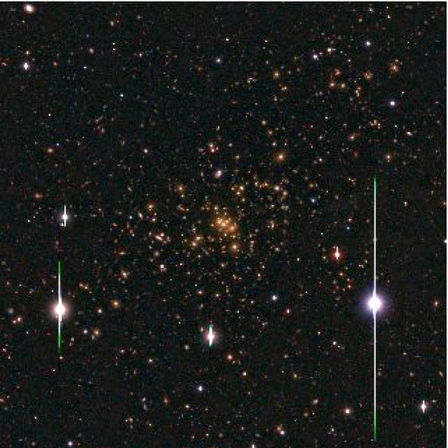
Figure 1.— Subaru $BRz^{\prime}$ pseudo-color image of the central $8\arcmin\times 8\arcmin$ region of the galaxy cluster Cl0024+1654 at $z=0.395$. The side length of the field is $1.8$ Mpc $h^{-1}$ at the cluster redshift.

Figure 2.— The quadrupole PSF anisotropy field as measured from stellar ellipticities before and after the PSF anisotropy correction. The left panel shows the raw ellipticity field of stellar objects, and the right panel shows the residual ellipticity field after the PSF anisotropy correction. The orientation of the sticks indicates the position angle of the major axis of stellar ellipticity, whereas the length is proportional to the modulus of stellar ellipticity. A stick with the length of $5\%$ ellipticity is indicated in the top right of the right panel.

Figure 3.— Stellar ellipticity distributions before and after the PSF anisotropy correction. The left panel shows the raw ellipticity components $(e_{1}^{*},e_{2}^{*})$ of stellar objects, and the right panel shows the residual ellipticity components $(\delta e_{1}^{*},\delta e_{2}^{*})$ after the PSF anisotropy correction.

Figure 4.— Mean statistical weight $u_{g}$ as measured from the magnitude-selected galaxy sample, shown as a function of the object Gaussian size $r_{g}$ (left) and of the $R_{\rm c}$ magnitude (right). In each of the panels, the statistical weight $u_{g}$ is normalized to unity in the first bin.

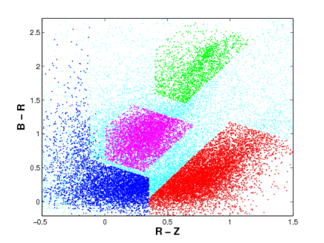
Figure 5.— Sample selection in the color-color diagram of Cl0024+1654, displaying the green sample (green points), comprising mostly cluster member galaxies, and the red (red points) and blue (blue points) samples, comprising of background galaxies. The galaxies that we identify as predominantly foreground lie in between the cluster and background galaxies are marked in magenta.

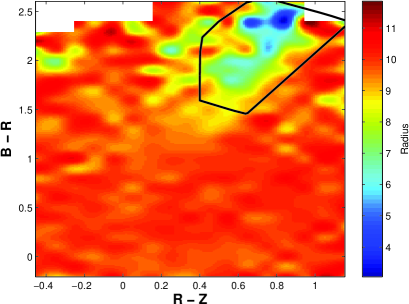
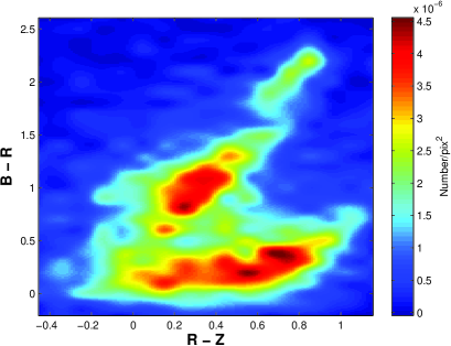
Figure 6.— Left: Distribution of mean projected distances from the cluster center for all galaxies in the Cl0024+1654 field, displayed in color-color (CC) space. The bluer colors imply smaller mean radii, hence correspond to the location of the cluster in CC space. The black box marks the boundaries of the green galaxy sample we select which conservatively includes all cluster members. Right: Number density of galaxies in CC space. Several distinct density peaks are shown to be different galaxy populations - the reddest peak in the upper-right corner of the plot depicts the overdensity of cluster galaxies, whose colors are lying on the red sequence; the middle peak with colors bluer than the cluster shows the overdensity of foreground galaxies; the remaining peaks in the bottom part (bluest in $B-R_{\rm c}$) can be demonstrated to comprise of blue and red (left and right, respectively) background galaxies.

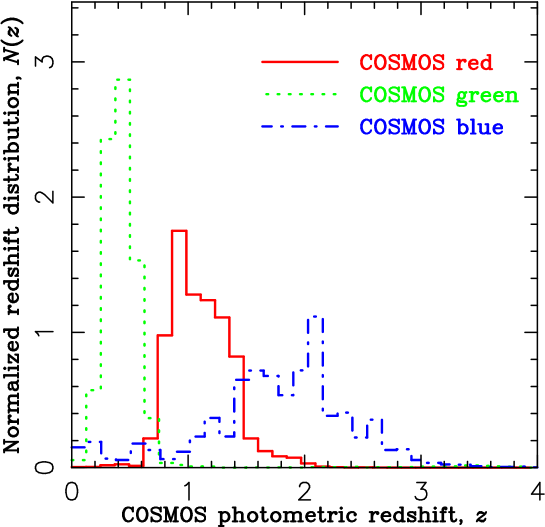
Figure 7.— Photometric redshift distributions $N(z)$ of $BR_{\rm c}z^{\prime}$ selected galaxy samples in the 2-deg² COSMOS field. The green (green dotted line), red (red solid line), and blue (blue dotted-dashed line) galaxy samples are selected according to color-color/magnitude limits used in the weak-lensing analysis of Cl0024+1654. Each distribution is normalized by $\int\!dz\,N(z)=1$.

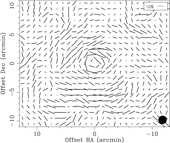
Figure 8.— Gravitational reduced-shear field in Cl0024+1654 obtained from shape distortions of the blue+red background galaxies, smoothed with a Gaussian with ${\rm FWHM}=1.4\arcmin$ for visualization purposes. A stick with a length of $10\%$ shear is indicated in the top right corner. The filled circle indicates the FWHM of the Gaussian. The coordinate origin is at the center of the cD galaxy.

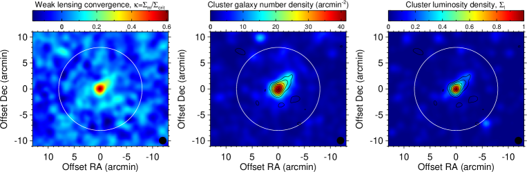
Figure 9.— Comparison of the surface mass density field and the cluster galaxy distributions in Cl0024+1654. Left: Dimensionless surface mass density field, or the lensing convergence $\kappa(\mbox{\boldmath$\theta$})=\Sigma_{m}(\mbox{\boldmath$\theta$})/\Sigma_{\rm crit}$, reconstructed from Subaru distortion data. Middle: Observed surface number density distribution $\Sigma_{n}(\mbox{\boldmath$\theta$})$ of $BR_{\rm c}z^{\prime}$-selected green galaxies ($17.3<z^{\prime}<25.5$ AB mag), representing unlensed cluster member galaxies. Right: Observed $R_{\rm c}$-band surface luminosity density distribution $\Sigma_{l}(\mbox{\boldmath$\theta$})$ of the same cluster membership. The solid circle in each panel indicates the cluster virial radius of $\theta_{\rm vir}\simeq 8\arcmin$, or $r_{\rm vir}\simeq 1.8$ Mpc $h^{-1}$ at the cluster redshift of $z=0.395$. All images are smoothed with a circular Gaussian of FWHM $1.4\arcmin$. Also overlaid on the $\Sigma_{n}(\mbox{\boldmath$\theta$})$ and $\Sigma_{l}(\mbox{\boldmath$\theta$})$ maps are the $\kappa(\mbox{\boldmath$\theta$})$ field shown in the left panel, given in units of $2\sigma$ reconstruction error from the lowest contour level of $3\sigma$. The field size is $26\arcmin\times 22\arcmin$. North is to the top, east to the left.

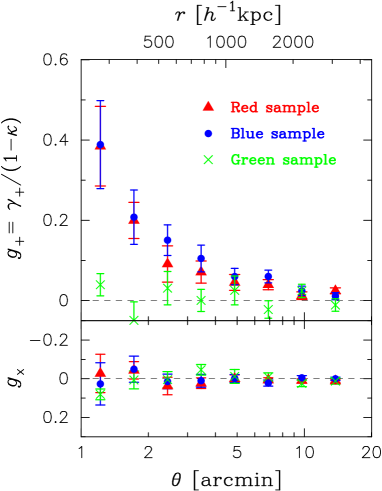
Figure 10.— Azimuthally-averaged radial profiles of the tangential reduced shear $g_{+}$ (upper panel) and the $45^{\circ}$ rotated ($\times$) component $g_{\times}$ (lower panel) for our red (triangles), blue (circles), and green (crosses), galaxy samples. The error bars represent $68.3\%$ confidence intervals estimated by bootstrap resampling techniques. The red and blue populations show a very similar form of the radial distortion profile which declines smoothly from the cluster center, remaining positive to the limit of our data, $\theta_{\rm max}=16\arcmin$. For all of the samples, the $\times$-component is consistent with a null signal at all radii, indicating the reliability of our distortion analysis.

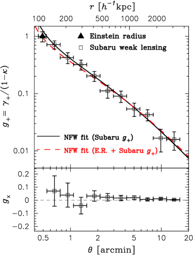
Figure 11.— Azimuthally-averaged radial profile of the tangential reduced shear $g_{+}$ (upper panel) as measured from Subaru distortion data of our composite blue+red background sample. The Einstein radius constraint (triangle) of $\theta_{\rm E}=30\arcsec\pm 3\arcsec$ (at $z_{s}=1.675$), determined from multiply lensed images in HST/ACS/NIC3 observations (Zitrin et al., 2009b), is translated to the corresponding depth of the Subaru blue+red background sample (Table 3), using the best-fit NFW model to the Subaru and ACS/NIC3 data (see Figure 14), and added to the distortion profile ($g_{+}=1$), marking the point of maximum distortion. The solid curve shows the best-fit NFW profile for the Subaru $g_{+}$ measurements. The dashed curve shows the NFW profile from a joint fit to the inner Einstein-radius constraint and the outer Subaru $g_{+}$ profile. Shown in the bottom panel is the $45^{\circ}$-rotated $g_{\times}$ component.

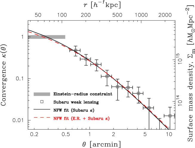
Figure 12.— Radial profile of lensing convergence $\kappa(\theta)=\Sigma_{m}(\theta)/\Sigma_{\rm crit}$ as reconstructed from Subaru distortion data. The open squares show the results from a non-linear extension of aperture mass densitometry based on azimuthally-averaged tangential distortion measurements. The error bars are correlated. The gray-shaded region represents the Einstein-radius constraint on the mean interior convergence, $\bar{\kappa}(<\theta_{\rm E})=1$, translated into the corresponding depth of the Subaru blue+red background sample. The dashed and solid curves are the best-fitting NFW profiles from the Subaru $\kappa$ data with and without the inner Einstein radius constraint combined, respectively.

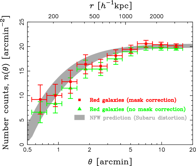
Figure 13.— Number-count profile of $BR_{\rm c}z^{\prime}$-selected red galaxies (squares) in the background of Cl0024+1654. The triangles show the counts without the mask correction due to cluster members and bright foreground objects. The gray-filled region represents the $68.3\%$ confidence bounds for the predicted count depletion curve from an NFW model constrained by our Subaru distortion analysis, demonstrating clear consistency between these two independent lensing observables.

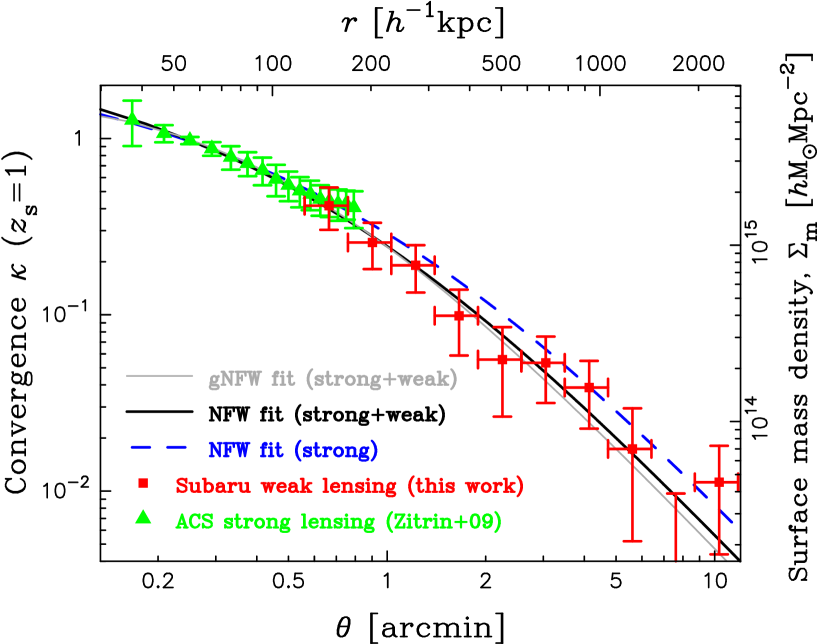
Figure 14.— Radial surface mass density profile of the galaxy cluster Cl0024+1654 over a wide range of radius from 40 to 2300 kpc$\,h^{-1}$ reconstructed from our joint weak and strong lensing analysis of Subaru and ACS/NIC3 observations. All of the radial profiles are scaled to a fiducial redshift of $z_{s}=1$. The squares represent our Subaru results (this work) from a one-dimensional reconstruction by a non-linear extension of aperture mass densitometry based on azimuthally-averaged tangential distortion measurements. The error bars are correlated. The triangles represent the inner $\kappa$ profile derived from the strong-lensing analysis of Zitrin et al. (2009b) based on 33 multiply-lensed images, spread fairly evenly over the central region, $8\arcsec\lower 2.15277pt\hbox{$\;\buildrel<\over{\sim}\;$}\theta\lower 2.15277pt\hbox{$\;\buildrel<\over{\sim}\;$}48\arcsec$. The thick (black) and thin (gray) solid curves show the best-fitting NFW and gNFW profiles, respectively, from our full lensing analysis of ACS/NIC3 and Subaru observations. The best-fitting NFW profile from the inner $\kappa$ profile from the ACS/NIC3 observations is also shown as a (blue) dashed curve. The Subaru weak-lensing constraint at the innermost radius is fully consistent with the strong-lensing information within the measurement uncertainty.

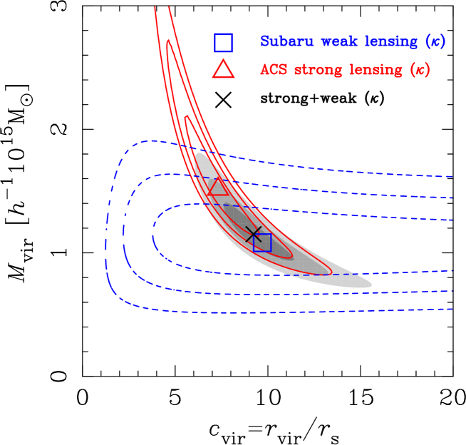
Figure 15.— Joint constraints on the NFW model parameters $(c_{\rm vir},M_{\rm vir})$ for Cl0024+1654 derived from the radial profile of lensing convergence, $\kappa(\theta)=\Sigma_{m}(\theta)/\Sigma_{\rm crit}$ (see Figure 14). The open square shows the best-fit set of the NFW model parameters, and the dashed contours show the 68.3%, 95.4%, and 99.7% confidence levels in the $c_{\rm vir}$-$M_{\rm vir}$ plane. The solid contours show the same confidence levels, but for an NFW fit to the inner ($10\arcsec\lower 2.15277pt\hbox{$\;\buildrel<\over{\sim}\;$}\theta\lower 2.15277pt\hbox{$\;\buildrel<\over{\sim}\;$}48\arcsec$) $\kappa$ profile constrained by deep ACS/NIC3 observations of Zitrin et al. (2009b). The corresponding best-fit set of $(c_{\rm vir},M_{\rm vir})$ is shown by the open triangle. Also shown by the filled gray areas are the same confidence areas, but obtained for a joint fit to the combined ACS/NIC3 and Subaru $\kappa(\theta)$ data. The corresponding best-fit set of $(c_{\rm vir},M_{\rm vir})$ is shown by the cross.

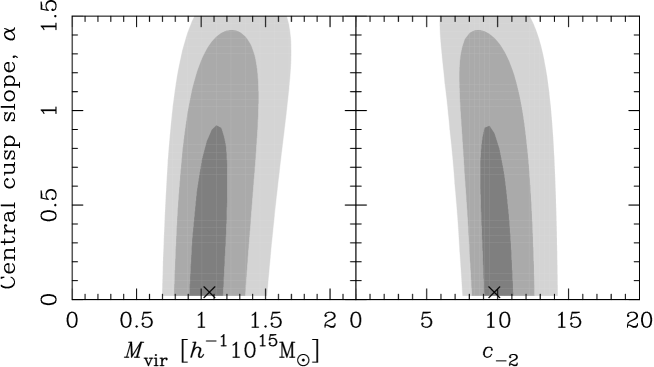
Figure 16.— Constraint on the the gNFW model parameters, namely the central cusp slope $\alpha$, the halo virial mass $M_{\rm vir}$, and the halo concentration $c_{-2}=c_{\rm vir}/(2-\alpha)$, when all of them are allowed to vary, derived from the full lensing profile of CL0024+1654 shown in Figure 14. The left and right panels show the two-dimensional marginalized constraints on $(M_{\rm vir},\alpha)$ and $(c_{-2},\alpha)$, respectively. In each panel of the figure, the contours show the 68.3%, 95.4%, and 99.7% confidence levels, and the cross indicates the best-fit model parameters.

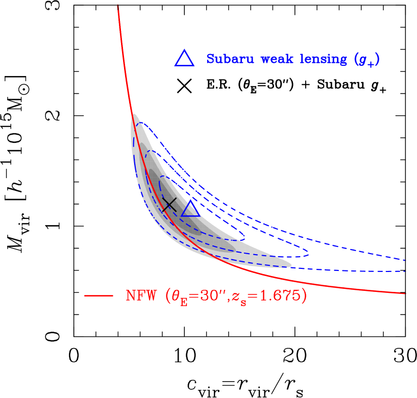
Figure 17.— Joint constraints on the NFW model parameters $(c_{\rm vir},M_{\rm vir})$ derived from Subaru distortion data. The dashed contours show the 68.3%, 95.4%, and 99.7% confidence levels in the $c_{\rm vir}$-$M_{\rm vir}$ plane, estimated from $\Delta\chi^{2}\equiv\chi^{2}-\chi^{2}_{\rm min}=2.3,6.17$, and $11.8$, respectively, for the tangential distortion ($g_{+}$) profile (Figure 11). Also shown by the filled gray areas are the same confidence regions, but obtained for a joint fit to the outer Subaru $g_{+}$ profile and the strong-lensing constraint on the location of the Einstein radius, $\theta_{\rm E}=30\arcsec\pm 3\arcsec$ at $z_{s}=1.675$. The open triangle shows the best-fit set of the NFW model parameters, $(c_{\rm vir},M_{\rm vir})$, for the Subaru $g_{+}$ results. The cross shows the best-fit set of $(c_{\rm vir},M_{\rm vir})$ for the combined Subaru $g_{+}$ and Einstein-radius constraints. The solid curve shows the NFW $c_{\rm vir}$-$M_{\rm vir}$ relation for $\theta_{\rm E}=30\arcsec$ at $z_{s}=1.675$.

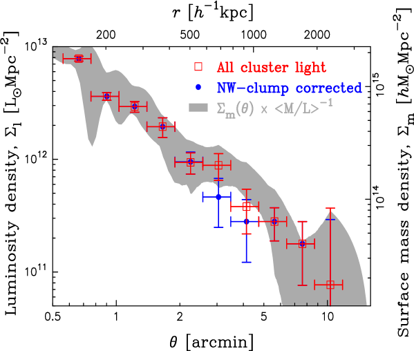
Figure 18.— The $R_{\rm c}$-band surface luminosity density profile $\Sigma_{l}(\theta)$ (squares) of $BR_{\rm c}z^{\prime}$-selected cluster member galaxies in Cl0024+1654. The gray-filled region represents the 68.3% confidence bounds for the surface mass density profile $\Sigma_{m}(\theta)$ reconstructed from our joint weak and strong lensing analysis (Figure 14), converted into a luminosity density assuming a constant mass-to-light ratio of $\langle M/L_{R}\rangle(<3\arcmin)\simeq 230h\,(M/L_{R})_{\odot}$. Also shown with filled circles is the same cluster luminosity density profile, but corrected for the presence of the northwest clump located at a projected distance of $\theta\sim 3\arcmin$.

Figure 19.— Model-independent radial profile of the differential mass-to-light ratio $\delta M(\theta)/\delta L_{R}(\theta)=\Sigma_{m}(\theta)/\Sigma_{l}(\theta)$ derived using the surface mass density profile $\Sigma_{m}(\theta)$ (see Figure 12) from the Subaru weak-lensing analysis and the $K$-corrected $R_{\rm c}$-band surface luminosity density profile $\Sigma_{l}(\theta)$ measured from $BR_{\rm c}z^{\prime}$-selected cluster member galaxies. The error bars represent 68.3% confidence limits.

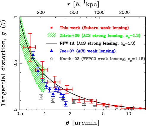
Figure 20.— Comparison of tangential distortion ($g_{+}$) profiles from different lensing studies. No correction is applied to the mean depth of lensing observations between different studies. The hatched region shows the $68.3\%$ confidence interval for the ACS strong-lensing results based on the azimuthally-averaged $\kappa$ profile of Zitrin et al. (2009b), scaled to a source redshift of $z_{s}=1.3$, roughly matching the mean depth of the Subaru blue+red background sample (see Table 3). Also shown with the solid curve is the best-fit NFW model ($z_{s}=1.3$) from the ACS strong lensing constraints. The squares show our Subaru $g_{+}$ profile as measured from $BR_{\rm c}z^{\prime}$-selected blue+red background galaxies. A simple extrapolation of the ACS/NIC3-derived NFW profile (solid curve) fits well with the outer Subaru distortion information (squares) over a wide range of radius, but somewhat overpredicts the distortion profile at $3\arcmin\lower 2.15277pt\hbox{$\;\buildrel<\over{\sim}\;$}\theta\lower 2.15277pt\hbox{$\;\buildrel<\over{\sim}\;$}5\arcmin$. The triangles show the $g_{+}$ profile from the weak lensing analysis of Jee et al. (2007, Figure 13) based on deep 6-passband HST/ACS images, where the data are limited to the positive parity region ($\theta\lower 2.15277pt\hbox{$\;\buildrel>\over{\sim}\;$}40\arcsec$) in this comparison. The open circles show the $g_{+}$ profile at $0.9\arcmin\lower 2.15277pt\hbox{$\;\buildrel<\over{\sim}\;$}\theta\lower 2.15277pt\hbox{$\;\buildrel<\over{\sim}\;$}11\arcmin$ from the weak lensing analysis of Kneib et al. (2003, Figure 7) based on a sparse-sampled mosaic of 2-band (F450W, F814W) WFPC2 observations. The flattened slope of Kneib et al. $g_{+}$ profile ($\overline{z}_{s}=1.15\pm 0.3$) at $\theta\lower 2.15277pt\hbox{$\;\buildrel<\over{\sim}\;$}2\arcmin$ is likely due to contamination of the weak lensing signal by unlensed cluster member galaxies. Note that Kneib et al. (2003) made a correction for this dilution effect in their two-dimensional lens modelling.

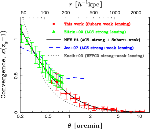
Figure 21.— Comparison of projected mass density ($\kappa$) profiles of Cl0024+1654 from different lensing studies. All of the radial profiles are scaled to a fiducial redshift of $z_{s}=1$. The squares represent our model-independent $\kappa(\theta)$ profile (this work) reconstructed from Subaru distortion data (Figure 12). The error bars are correlated. The triangles represent the results from the strong-lensing analysis of Zitrin et al. (2009b) based on deep ACS/NIC3 images. The solid curve shows the best-fitting NFW profile from our full lensing analysis of ACS/NIC3 and Subaru observations covering a wide range of radii, $R\simeq[40,2300]$ kpc$\,h^{-1}$. The dashed curve shows the $\kappa$ profile ($\theta\lower 2.15277pt\hbox{$\;\buildrel<\over{\sim}\;$}1.8\arcmin$) reconstructed from the ACS weak and strong lensing analysis of Jee et al. (2007). The dotted curve shows the two-component lens mass model constrained from the WFPC2 weak lensing measurements of Kneib et al. (2003) combined with the inner strong-lensing constraint on the Einstein radius.

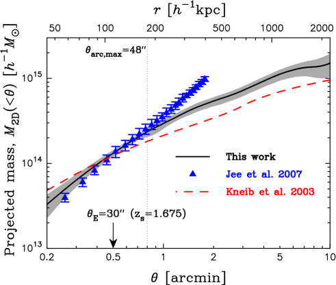
Figure 22.— Comparison of cumulative projected mass profiles $M_{\rm 2D}(<\theta)$ of the galaxy cluster Cl0024+1654 from different lensing studies. The solid curve (this work) represents the results from our joint weak and strong lensing analysis of deep Subaru and ACS/NIC3 observations over a wide radial range from $40$ kpc $h^{-1}$ to $2300$ kpc $h^{-1}$. The gray-shaded area shows the $68.3\%$ confidence interval at each radius estimated from a Monte-Carlo error analysis taking into account the error covariance matrix of our full lensing constraints. Shown with a dotted vertical line is the maximum radius of multiply-lensed images used in the strong lensing analysis of Zitrin et al. (2009b). The triangles represent the results from the ACS weak lensing analysis of Jee et al. (2007, Figure 12). The dashed curve shows the best-fit two-component lens model of Kneib et al. (2003), constrained from their WFPC2 weak lensing measurements combined with the inner Einstein radius constraint, taking into account the contribution of both the central and northwest clumps identified in projection space. The three mass profiles from different lensing work are in good agreement at the Einstein radius $\theta_{\rm E}\simeq 30\arcsec$ (as indicated by the arrow) for the 5-image system ($z_{s}=1.675$), by which each profile is normalized. The projected mass profile of Jee et al. (2007) is in an excellent agreement with our joint mass profile out to $\theta\simeq 1.1\arcmin$ ($r\simeq 250$ kpc $h^{-1}$ in projection space), but increasingly exceeds our profile at $\theta\lower 2.15277pt\hbox{$\;\buildrel>\over{\sim}\;$}1.1\arcmin$ out to the limit of their data.

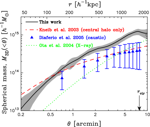
Figure 23.— Comparison of cumulative spherical mass profiles $M_{\rm 3D}(<\theta)$ of the galaxy cluster Cl0024+1654 from different studies. The solid curve (this work) represents the deprojected spherical mass profile from our full lensing analysis of Subaru and ACS/NIC3 data assuming spherical symmetry for the cluster system. The gray shaded area shows the $68.3\%$ confidence interval at each radius estimated from a Monte-Carlo error analysis taking into account the error covariance matrix of our joint Subaru and ACS/NIC3 lensing constraints. Shown with a dashed curve is the spherical NFW model of Kneib et al. (2003) for the central component alone (see also Figure 22). The triangles represent the results from the dynamical analysis of Diaferio et al. (2005) based on the caustic method. The dotted curve shows the best-fitting NFW profile from the Chandra X-ray analysis of Ota et al. (2004) obtained assuming the hydrostatic equilibrium. Note that the maximum limit of the Chandra data of Ota et al. (2004) is about $4\arcmin$ ($900$ kpc $h^{-1}$). Our joint mass profile is only marginally consistent with the dynamical results of Diaferio et al. (2005) out to $\theta\sim 3.5\arcmin$, but increasingly exceeds the caustic-based profile at large radii. A significant increase in $M_{\rm 3D}(<r)$ is seen in our joint mass profile at $3.5\arcmin\lower 2.15277pt\hbox{$\;\buildrel<\over{\sim}\;$}\theta\lower 2.15277pt\hbox{$\;\buildrel<\over{\sim}\;$}5\arcmin$, indicating an additional, extended mass component in the outer radius.

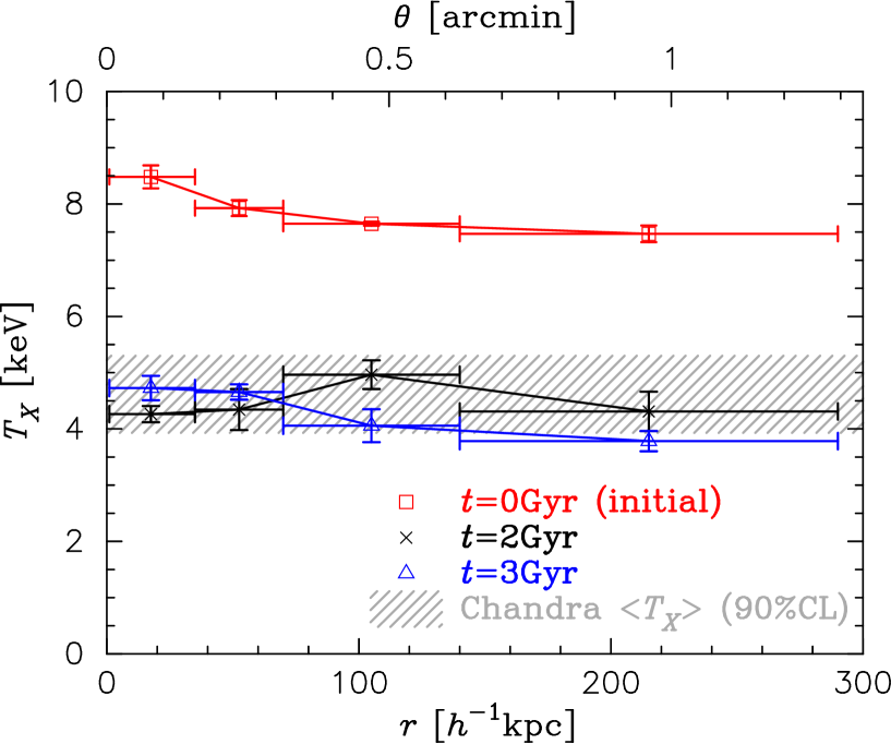
Figure 24.— Projected spectroscopic-like temperature profiles created from mock X-ray observations of our simulated head-on 2:1 mass-ratio cluster merger, shown at three different times, $t=0,2$, and $3$ Gyr after the beginning of the collision (open squares, crosses, and open triangles, respectively). The vertical error bars represent the dispersion due to azimuthal averaging. The hatched region shows the 90% confidence interval for the average X-ray temperature, $T_{X}=4.47^{+0.83}_{-0.54}$, from Chandra X-ray observations of Ota et al. (2004).

References

- Baltz et al. (2007) Baltz, E. A., Marshall, P., & Oguri, M. 2007, ArXiv e-prints, 705, 0705.0682
- Bartelmann (1996) Bartelmann, M. 1996, A&A, 313, 697, arXiv:astro-ph/9602053
- Bartelmann & Schneider (2001) Bartelmann, M., & Schneider, P. 2001, Phys. Rep., 340, 291, arXiv:astro-ph/9912508
- Benítez (2000) Benítez, N. 2000, ApJ, 536, 571
- Bertin (2006) Bertin, E. 2006, in Astronomical Society of the Pacific Conference Series, Vol. 351, Astronomical Data Analysis Software and Systems XV, ed. C. Gabriel, C. Arviset, D. Ponz, & S. Enrique, 112–+
- Bertin & Arnouts (1996) Bertin, E., & Arnouts, S. 1996, A&AS, 117, 393
- Blumenthal et al. (1986) Blumenthal, G. R., Faber, S. M., Flores, R., & Primack, J. R. 1986, ApJ, 301, 27
- Bolzonella et al. (2000) Bolzonella, M., Miralles, J.-M., & Pelló, R. 2000, A&A, 363, 476, arXiv:astro-ph/0003380
- Broadhurst et al. (2005a) Broadhurst, T. et al. 2005a, ApJ, 621, 53, arXiv:astro-ph/0409132
- Broadhurst et al. (2000) Broadhurst, T., Huang, X., Frye, B., & Ellis, R. 2000, ApJ, 534, L15, arXiv:astro-ph/9902316
- Broadhurst et al. (2005b) Broadhurst, T., Takada, M., Umetsu, K., Kong, X., Arimoto, N., Chiba, M., & Futamase, T. 2005b, ApJ, 619, L143, arXiv:astro-ph/0412192
- Broadhurst et al. (2008) Broadhurst, T., Umetsu, K., Medezinski, E., Oguri, M., & Rephaeli, Y. 2008, ApJ, 685, L9, 0805.2617
- Broadhurst & Barkana (2008) Broadhurst, T. J., & Barkana, R. 2008, MNRAS, 390, 1647, 0801.1875
- Broadhurst et al. (1995) Broadhurst, T. J., Taylor, A. N., & Peacock, J. A. 1995, ApJ, 438, 49, arXiv:astro-ph/9406052
- Capak et al. (2007) Capak, P. et al. 2007, ApJS, 172, 99, arXiv:0704.2430
- Clowe et al. (2006) Clowe, D., Bradač, M., Gonzalez, A. H., Markevitch, M., Randall, S. W., Jones, C., & Zaritsky, D. 2006, ApJ, 648, L109, arXiv:astro-ph/0608407
- Clowe et al. (2000) Clowe, D., Luppino, G. A., Kaiser, N., & Gioia, I. M. 2000, ApJ, 539, 540, arXiv:astro-ph/0001356
- Coe et al. (2006) Coe, D., Benítez, N., Sánchez, S. F., Jee, M., Bouwens, R., & Ford, H. 2006, AJ, 132, 926, arXiv:astro-ph/0605262
- Colella & Woodward (1984) Colella, P., & Woodward, P. R. 1984, Journal of Computational Physics, 54, 174
- Colley et al. (1996) Colley, W. N., Tyson, J. A., & Turner, E. L. 1996, ApJ, 461, L83+, arXiv:astro-ph/9512128
- Comerford et al. (2006) Comerford, J. M., Meneghetti, M., Bartelmann, M., & Schirmer, M. 2006, ApJ, 642, 39, arXiv:astro-ph/0511330
- Comerford & Natarajan (2007) Comerford, J. M., & Natarajan, P. 2007, MNRAS, 379, 190, arXiv:astro-ph/0703126
- Crittenden et al. (2002) Crittenden, R. G., Natarajan, P., Pen, U.-L., & Theuns, T. 2002, ApJ, 568, 20, arXiv:astro-ph/0012336
- Czoske et al. (2001) Czoske, O., Kneib, J.-P., Soucail, G., Bridges, T. J., Mellier, Y., & Cuillandre, J.-C. 2001, A&A, 372, 391, arXiv:astro-ph/0103123
- Czoske et al. (2002) Czoske, O., Moore, B., Kneib, J.-P., & Soucail, G. 2002, A&A, 386, 31, arXiv:astro-ph/0111118
- Diaferio (1999) Diaferio, A. 1999, MNRAS, 309, 610, arXiv:astro-ph/9906331
- Diaferio et al. (2005) Diaferio, A., Geller, M. J., & Rines, K. J. 2005, ApJ, 628, L97, arXiv:astro-ph/0506560
- Dressler et al. (1999) Dressler, A., Smail, I., Poggianti, B. M., Butcher, H., Couch, W. J., Ellis, R. S., & Oemler, A. J. 1999, ApJS, 122, 51, arXiv:astro-ph/9901263
- Duffy et al. (2008) Duffy, A. R., Schaye, J., Kay, S. T., & Dalla Vecchia, C. 2008, MNRAS, 390, L64, 0804.2486
- Erben et al. (2001) Erben, T., Van Waerbeke, L., Bertin, E., Mellier, Y., & Schneider, P. 2001, A&A, 366, 717, arXiv:astro-ph/0007021
- Fahlman et al. (1994) Fahlman, G., Kaiser, N., Squires, G., & Woods, D. 1994, ApJ, 437, 56, arXiv:astro-ph/9402017
- Ford et al. (2003) Ford, H. C. et al. 2003, in Presented at the Society of Photo-Optical Instrumentation Engineers (SPIE) Conference, Vol. 4854, Society of Photo-Optical Instrumentation Engineers (SPIE) Conference Series, ed. J. C. Blades & O. H. W. Siegmund, 81–94
- Fryxell et al. (2000) Fryxell, B. et al. 2000, ApJS, 131, 273
- Goldberg & Bacon (2005) Goldberg, D. M., & Bacon, D. J. 2005, ApJ, 619, 741, arXiv:astro-ph/0406376
- Hamana et al. (2003) Hamana, T. et al. 2003, ApJ, 597, 98, arXiv:astro-ph/0210450
- Hennawi et al. (2007) Hennawi, J. F., Dalal, N., Bode, P., & Ostriker, J. P. 2007, ApJ, 654, 714, arXiv:astro-ph/0506171
- Heymans et al. (2006) Heymans, C. et al. 2006, MNRAS, 368, 1323, arXiv:astro-ph/0506112
- Hoekstra (2007) Hoekstra, H. 2007, MNRAS, 379, 317, arXiv:0705.0358
- Hoekstra et al. (2000) Hoekstra, H., Franx, M., & Kuijken, K. 2000, ApJ, 532, 88, arXiv:astro-ph/9910487
- Hoekstra et al. (1998) Hoekstra, H., Franx, M., Kuijken, K., & Squires, G. 1998, ApJ, 504, 636
- Ilbert et al. (2009) Ilbert, O. et al. 2009, ApJ, 690, 1236, 0809.2101
- Jain et al. (2000) Jain, B., Seljak, U., & White, S. 2000, ApJ, 530, 547, arXiv:astro-ph/9901191
- Jee et al. (2007) Jee, M. J. et al. 2007, ApJ, 661, 728, 0705.2171
- Jing & Suto (2000) Jing, Y. P., & Suto, Y. 2000, ApJ, 529, L69, arXiv:astro-ph/9909478
- Kaiser (1995) Kaiser, N. 1995, ApJ, 439, L1, arXiv:astro-ph/9408092
- Kaiser & Squires (1993) Kaiser, N., & Squires, G. 1993, ApJ, 404, 441
- Kaiser et al. (1995) Kaiser, N., Squires, G., & Broadhurst, T. 1995, ApJ, 449, 460, arXiv:astro-ph/9411005
- Kassiola et al. (1992) Kassiola, A., Kovner, I., & Fort, B. 1992, ApJ, 400, 41
- Kneib et al. (2003) Kneib, J.-P. et al. 2003, ApJ, 598, 804, arXiv:astro-ph/0307299
- Kodama et al. (2005) Kodama, T. et al. 2005, PASJ, 57, 309, arXiv:astro-ph/0502444
- Koo (1988) Koo, D. C. 1988, Recent observations of distant matter - Direct clues to birth and evolution, ed. V. C. Rubin & G. V. Coyne, 513–540
- Kravtsov et al. (2006) Kravtsov, A. V., Vikhlinin, A., & Nagai, D. 2006, ApJ, 650, 128, arXiv:astro-ph/0603205
- Lapi & Cavaliere (2009) Lapi, A., & Cavaliere, A. 2009, ApJ, 695, L125, 0903.1589
- Lemze et al. (2008) Lemze, D., Barkana, R., Broadhurst, T. J., & Rephaeli, Y. 2008, MNRAS, 386, 1092, arXiv:0711.3908
- Lemze et al. (2009) Lemze, D., Broadhurst, T., Rephaeli, Y., Barkana, R., & Umetsu, K. 2009, ApJ, 701, 1336, arXiv:astr-ph/0810.3129
- Liesenborgs et al. (2008a) Liesenborgs, J., de Rijcke, S., Dejonghe, H., & Bekaert, P. 2008a, MNRAS, 386, 307, 0801.4255
- Liesenborgs et al. (2008b) ——. 2008b, MNRAS, 389, 415, 0806.2609
- Mahdavi et al. (2008) Mahdavi, A., Hoekstra, H., Babul, A., & Henry, J. P. 2008, MNRAS, 384, 1567, 0710.4132
- Massey et al. (2007) Massey, R. et al. 2007, MNRAS, 376, 13, arXiv:astro-ph/0608643
- Mazzotta et al. (2004) Mazzotta, P., Rasia, E., Moscardini, L., & Tormen, G. 2004, MNRAS, 354, 10, arXiv:astro-ph/0409618
- Medezinski et al. (2007) Medezinski, E. et al. 2007, ApJ, 663, 717, arXiv:astro-ph/0608499
- Medezinski et al. (2009) Medezinski, E., Broadhurst, T., Umetsu, K., Oguri, M., Rephaeli, Y., & Benítez, N. 2009, ApJ, in press, arXiv:0906.4791
- Miyazaki et al. (2002) Miyazaki, S. et al. 2002, PASJ, 54, 833, arXiv:astro-ph/0211006
- Navarro et al. (1997) Navarro, J. F., Frenk, C. S., & White, S. D. M. 1997, ApJ, 490, 493, arXiv:astro-ph/9611107
- Neto et al. (2007) Neto, A. F. et al. 2007, MNRAS, 381, 1450, arXiv:0706.2919
- Newman et al. (2009) Newman, A. B., Treu, T., Ellis, R. S., Sand, D. J., Richard, J., Marshall, P. J., Capak, P., & Miyazaki, S. 2009, ApJ, 706, 1078, 0909.3527
- Oguri & Blandford (2009) Oguri, M., & Blandford, R. D. 2009, MNRAS, 392, 930, arXiv:astro-ph/0808.0192
- Oguri et al. (2009) Oguri, M. et al. 2009, ApJ, 699, 1038, arXiv:astro-ph/0901.4372
- Okabe et al. (2009) Okabe, N., Takada, M., Umetsu, K., Futamase, T., & Smith, G. P. 2009, ArXiv e-prints, arXiv:astro-ph/0903.1103
- Okabe & Umetsu (2008) Okabe, N., & Umetsu, K. 2008, PASJ, 60, 345, arXiv:astro-ph/0702649
- Okura et al. (2007) Okura, Y., Umetsu, K., & Futamase, T. 2007, ApJ, 660, 995, arXiv:astro-ph/0607288
- Okura et al. (2008) ——. 2008, ApJ, 680, 1, arXiv:0710.2262
- Ota et al. (2004) Ota, N., Pointecouteau, E., Hattori, M., & Mitsuda, K. 2004, ApJ, 601, 120, arXiv:astro-ph/0306580
- Ouchi et al. (2004) Ouchi, M. et al. 2004, ApJ, 611, 660, arXiv:astro-ph/0309655
- Park et al. (2003) Park, C.-G., Ng, K.-W., Park, C., Liu, G.-C., & Umetsu, K. 2003, ApJ, 589, 67, arXiv:astro-ph/0209491
- Richard et al. (2009) Richard, J., Pei, L., Limousin, M., Jullo, E., & Kneib, J. P. 2009, A&A, 498, 37, 0901.0427
- Ricker (2008) Ricker, P. M. 2008, ApJS, 176, 293, 0710.4397
- Ricker & Sarazin (2001) Ricker, P. M., & Sarazin, C. L. 2001, ApJ, 561, 621, arXiv:astro-ph/0107210
- Rines et al. (2000) Rines, K., Geller, M. J., Diaferio, A., Mohr, J. J., & Wegner, G. A. 2000, AJ, 120, 2338, arXiv:astro-ph/0007126
- Schneider et al. (2000) Schneider, P., King, L., & Erben, T. 2000, A&A, 353, 41, arXiv:astro-ph/9907143
- Schneider & Seitz (1995) Schneider, P., & Seitz, C. 1995, A&A, 294, 411, arXiv:astro-ph/9407032
- Seitz & Schneider (1997) Seitz, C., & Schneider, P. 1997, A&A, 318, 687, arXiv:astro-ph/9601079
- Shapiro & Iliev (2000) Shapiro, P. R., & Iliev, I. T. 2000, ApJ, 542, L1, arXiv:astro-ph/0006353
- Smail et al. (1996) Smail, I., Dressler, A., Kneib, J.-P., Ellis, R. S., Couch, W. J., Sharples, R. M., & Oemler, A. J. 1996, ApJ, 469, 508, arXiv:astro-ph/9503063
- Soucail et al. (2000) Soucail, G., Ota, N., Böhringer, H., Czoske, O., Hattori, M., & Mellier, Y. 2000, A&A, 355, 433, arXiv:astro-ph/9911062
- Takada & Jain (2003) Takada, M., & Jain, B. 2003, MNRAS, 340, 580, arXiv:astro-ph/0209167
- Tanaka et al. (2005) Tanaka, M., Kodama, T., Arimoto, N., Okamura, S., Umetsu, K., Shimasaku, K., Tanaka, I., & Yamada, T. 2005, MNRAS, 362, 268, arXiv:astro-ph/0506713
- Tyson et al. (1998) Tyson, J. A., Kochanski, G. P., & dell’Antonio, I. P. 1998, ApJ, 498, L107+, arXiv:astro-ph/9801193
- Umetsu et al. (2009) Umetsu, K. et al. 2009, ApJ, 694, 1643, arXiv:astro-ph/0810.0969
- Umetsu & Broadhurst (2008) Umetsu, K., & Broadhurst, T. 2008, ApJ, 684, 177, arXiv:0712.3441
- Umetsu et al. (1999) Umetsu, K., Tada, M., & Futamase, T. 1999, Progress of Theoretical Physics Supplement, 133, 53, arXiv:astro-ph/0004400
- Umetsu et al. (2007) Umetsu, K., Takada, M., & Broadhurst, T. 2007, Modern Physics Letters A, 22, 2099, arXiv:astro-ph/0702096
- Umetsu et al. (2005) Umetsu, K., Tanaka, M., Kodama, T., Tanaka, I., Futamase, T., Kashikawa, N., & Hoshi, T. 2005, PASJ, 57, 877, arXiv:astro-ph/0506746
- Vikhlinin et al. (2009) Vikhlinin, A. et al. 2009, ApJ, 692, 1033, 0805.2207
- Wright & Brainerd (2000) Wright, C. O., & Brainerd, T. G. 2000, ApJ, 534, 34
- Yagi et al. (2002) Yagi, M., Kashikawa, N., Sekiguchi, M., Doi, M., Yasuda, N., Shimasaku, K., & Okamura, S. 2002, AJ, 123, 66
- Zacharias et al. (2004) Zacharias, N., Monet, D. G., Levine, S. E., Urban, S. E., Gaume, R., & Wycoff, G. L. 2004, in Bulletin of the American Astronomical Society, Vol. 36, Bulletin of the American Astronomical Society, 1418–+
- Zhang et al. (2005) Zhang, Y.-Y., Böhringer, H., Mellier, Y., Soucail, G., & Forman, W. 2005, A&A, 429, 85, arXiv:astro-ph/0408545
- Zhao (1996) Zhao, H. 1996, MNRAS, 278, 488, arXiv:astro-ph/9509122
- Zheng et al. (2009) Zheng, W. et al. 2009, ApJ, 697, 1907, 0903.3988
- Zitrin & Broadhurst (2009) Zitrin, A., & Broadhurst, T. 2009, ApJ, 703, L132, 0906.5079
- Zitrin et al. (2009a) Zitrin, A., Broadhurst, T., Rephaeli, Y., & Sadeh, S. 2009a, ApJ, 707, L102, arXiv:astro-ph/0907.4232
- Zitrin et al. (2009b) Zitrin, A. et al. 2009b, MNRAS, 396, 1985, arXiv:0902.3971
- Zu Hone et al. (2009a) Zu Hone, J. A., Lamb, D. Q., & Ricker, P. M. 2009a, ApJ, 696, 694, 0809.3252
- Zu Hone et al. (2009b) Zu Hone, J. A., Ricker, P. M., Lamb, D. Q., & Karen Yang, H.-Y. 2009b, ApJ, 699, 1004, 0808.0930
- Zwicky (1959) Zwicky, F. 1959, Handbuch der Physik, 53, 390