High Velocity Molecular Outflow in CO $J=7-6$ Emission from the Orion Hot Core

Abstract

Using the Caltech Submillimeter Observatory 10.4-meter telescope, we performed sensitive mapping observations of ¹²CO $J=7-6$ emission at 807 GHz towards Orion IRc2. The image has an angular resolution of 10″, which is the highest angular resolution data toward the Orion Hot Core published for this transition. In addition, thanks to the on-the-fly mapping technique, the fidelity of the new image is rather high, particularly in comparison to previous images. We have succeeded in mapping the northwest-southeast high-velocity molecular outflow, whose terminal velocity is shifted by $\sim 70-85$ km s^-1 with respect to the systemic velocity of the cloud. This yields an extremely short dynamical time scale of $\sim$900 years. The estimated outflow mass loss rate shows an extraordinarily high value, on the order of $10^{-3}$ $M_{\odot}$ yr^-1. Assuming that the outflow is driven by Orion IRc2, our result agrees with the picture so far obtained for a 20 $M_{\odot}$ (proto)star in the process of formation.

1 Introduction

Despite its astrophysical importance, the high-mass ($M_{\ast}\mathrel{\hbox{\hbox to0.0pt{\hbox{\lower 4.0pt\hbox{$\sim$}}\hss}\hbox{$>$}}}8$ $M_{\odot}$) star formation process remains poorly understood both observationally and theoretically. High-velocity (HV) molecular outflows are the most prominent phenomena seen, not only in high-mass but also in low-mass star-forming regions. Molecular outflows from low-mass stars are thought to be momentum-driven by highly collimated stellar winds, and are closely related to the accretion process onto the central star (e.g., Arce et al. 2007, and references therein). Although such a paradigm cannot simply be scaled up to the high-mass regime, one may obtain important information about the formation mechanism of early-type stars by observing their outflows. In this context, the Orion Hot Core (HC) is the best site to study massive star formation process, as its proximity allows very detailed studies.

Ground-based mapping observations of CO lines at submillimeter (submm) wavelengths towards the region were pioneered by, e.g., Wilson et al. (2001) in the $J=7-6$ transition and Marrone et al. (2004) in $J=9-8$. These authors focused on studying the properties of the intense low-velocity gas around the velocity of the natal molecular cloud, which arises predominantly from a photo-dissociation region (PDR). Observations of low-$J$ lines, such as $J=2-1$, allow observers to attain high angular resolution images down to $\sim$1″ by utilizing interferometers, as demonstrated by Chernin & Wright (1996), Beuther & Nissen (2008), and others. However, such low-$J$ line observations of molecular outflows usually make it difficult to distinguish low-velocity outflowing gas from the quiescent ambient gas. The $J=7$ level is approximately 156 K above the ground-state level, and thus more sensitive to the presence of hot ($T>100$ K) gas. The Einstein A coefficient for the $J=7-6$ transition is 50 times greater than for the $J=2-1$ line, providing a high contrast between the warm and cold gas. Such characteristics greatly help us to distinguish HV outflowing gas from the surrounding material. To characterize the physical properties of the outflowing gas in the Orion HC, we performed observations of CO $J=7-6$ using the Caltech Submillimeter Observatory (CSO) 10.4-meter telescope, making full use of its high spatial and high spectral resolution.

2 Observations and Data Reduction

We carried out on-the-fly (OTF) mapping observations of the CO $J=$7–6 line (rest frequency, $\nu_{\rm rest}$ = 806651.720 MHz) with the CSO on 2009 January 21 and 22. The observations took 1–2 hrs each day. Prior to the submm observations, we performed optical pointing observations on 2009 January 20. Therefore, we believe that the overall pointing accuracy was better than 3″. We used the 850 GHz receiver (Kooi et al., 2000) with the Fast Fourier Transform Spectrometer (FFTS) as a back-end, yielding an effective velocity resolution ($\Delta v_{\rm res}$) of 0.0454 km s^-1 with the 1 GHz bandwidth mode. During the observations, the atmospheric zenith optical depth at 225 GHz ranged between 0.035 and 0.055, and the single side-band (SSB) system temperature ($T_{\rm sys}$) stayed between $\sim$2500 K and 8000 K, depending on the optical depth and the airmass. We wish to point out that our observations are almost twice as sensitive as the previous ¹²CO (7–6) observations by Wilson et al. (2001), whose typical $T_{\rm sys}$ was $\sim 14,000$ K. The OTF mapping was carried out over an area of $\sim 170\arcsec$ centered on Orion IRc2 (R.A. $=5^{h}35^{m}14.5^{s}$, Dec. $=-$5^∘ 22′ 30$\farcs$4 in B1950) by scanning once each along the R.A. and Dec. directions. Subsequently, we decided to concentrate on mapping the central 85″ region, which we further scanned twice along the R.A. and once along the Dec. directions. The OTF mapping scans were gridded with a pixel size scale of 5$\farcs$0 by employing a position-switching method. The telescope pointing was checked by observing the continuum emission towards Venus and Saturn every hour. At the line frequency, the beam size ($\theta_{\rm HPBW}$) is estimated to be 10″  and the main-beam efficiency ($\eta_{\rm mb}$) was 0.34 from our measurements towards Saturn. All the spectra were calibrated by the standard chopper wheel method, and were converted to main-beam brightness temperature ($T_{\rm mb}$) scale by dividing by $\eta_{\rm mb}$. The uncertainty in the intensity calibration is estimated to be $\sim$ 20%. After calibrating all the spectra, we made two 3D data cubes from two groups of the spectra taken by scanning along R.A. and Dec. directions. These two cubes were processed with the code “Basket-Weave”, implemented in the NOSTAR package (Sawada et al. 2007) to remove the scanning effect using the method developed by Emerson & Graeve (1988).

3 Results and Discussion

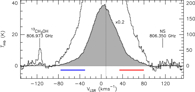
Figure 1: Single-dish spectra of the ¹²CO $7-6$ emission toward Orion IRc2 in the main-beam brightness temperature ($T_{\rm mb}$) scale with a velocity resolution of 0.726 km s^-1. See the $y$-axis labels of the right- and left-hand sides for the overall (filled histogram) and the magnified spectra, respectively. The RMS noise level is 0.72 K for 81 seconds integration. The blue- and red-colored horizontal bars below the spectra indicate the LSR-velocity ranges used to obtain the integrated intensity map shown in Figure 4. The systemic velocity of the cloud is $V_{\rm LSR}$ $\sim\,9$ km s^-1 which is indicated by the vertical dashed line.

Figure 1 shows our CO (7–6) spectrum towards Orion IRc2 in the $T_{\rm mb}$ scale. The spectral profile is rather broad, and shows prominent HV wing emission. The HV wing is seen both blue- and redshifted sides up to $\sim$80 km s^-1 away from the systemic velocity ($V_{\rm sys}$) of the cloud, $V_{\rm LSR}$$=9$ km s^-1. The peak $T_{\rm mb}$ is 202 K at $V_{\rm LSR}$$=\,1.9$ km s^-1, which is consistent with that measured by Comito et al. (2005), although the pointing centers differ between our maps and theirs by 5$\farcs$0. The CO spectrum shows a dip at $V_{\rm sys}$, suggesting that the line is optically thick around $V_{\rm sys}$. The two isolated emission lines can be seen at $V_{\rm LSR}$$\sim+110$ km s^-1 and $\sim-115$ km s^-1; they are identified as lines of NS ($f_{\rm rest}=$ 806350 MHz) and ¹³CH₃OH (806973 MHz), on the basis of the line survey (Comito et al., 2005) at the 350 µm band.

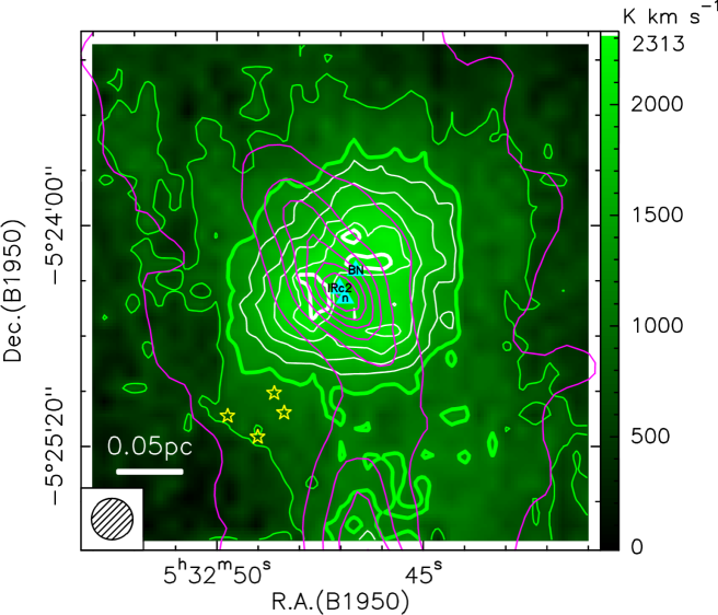
Figure 2: Overlay of the bulk emission of the ¹²CO (7–6) (green image plus white and green contours) on the 350 $\mu$m continuum emission (magenta contours; Lis et al. 1998). The contours for the ¹²CO (7–6) emission are the 95% level (thick white), 90%, 80%, 70%, 60% (thin white), 50% (thick green), and 30% (thin green) level of the peak for the clarity of the plot. The CO map is obtained by integrating the emission between $V_{\rm LSR}$$=$ 4.5 km s^-1 and 14.5 km s^-1. The light blue triangles with source names show the positions of the radio continuum sources [Menten & Reid (1995); Rodríguez et al. (2009)], and the yellow stars indicate the positions of the Trapezium members. Note that the peak position of the infrared source IRc2 is displaced from the radio source I by 0$\farcs$8 (Gezari, 1992). The hatched ellipse at the bottom left corner indicates the HPBW of the CSO beam (10″).

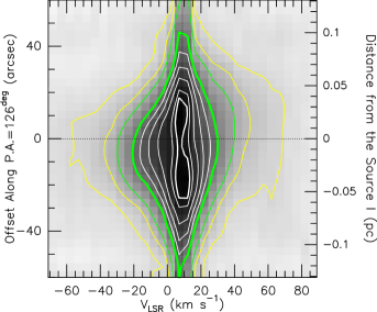
Figure 5: Position-velocity (PV) diagram of the ¹²CO (7–6) emission along the outflow axis (P.A.$=+126$^∘) passing through the position of IRc2 (see Figure 4). The white and green contours are the same as those in Figure 2, and the two yellow contours indicate the 20% and 10% levels with respect to the peak intensity. The vertical dashed-line at $V_{\rm LSR}$ $=$ 9 km s^-1 shows the $V_{\rm sys}$.

Figure 2 shows an overlay of the low-velocity bulk emission of the CO (7–6) and the 350 µm continuum emission (Lis et al., 1998). The (7–6) line shows intense emission surrounding IRc2, and spreads along the north-south direction if we consider the weak extended component. The CSO beam is too large to resolve the spatial separation of $\sim$0$\farcs$8 between IRc2 and Source I (Gezari, 1992) which has been proposed as a powering source for the Orion outflow (Beuther & Nissen 2008, and references therein). The north-south elongation of the weak emission corresponds to the Orion Ridge; the northern tip of the Orion South core can be recognized at the bottom (i.e., south) of our map. The widespread quiescent CO (7–6) emission is thought to be associated with the PDR heated by $\Theta^{1}C$ Orionis (Wilson et al., 2001). The bulk emission shows a condensation with a diameter of $\sim 80\arcsec$, measured at the 50% level contour, corresponding to 0.065 pc at $d=450$ pc. It should be noted that the CO (7–6) line and the 350 $\mu$m continuum emission do not show similar spatial structure; the former has a roundish shape, whereas the latter is elongated along the north-south direction. Another result deduced from Figure 2 is that the bulk emission does not show a single peak at the position of the 350 $\mu$m continuum peak. Instead, it shows two local maxima; one of them lies to the west of the BN object and the other is $\sim 10\arcsec$ east of IRc2. Positions of the two local maxima are roughly consistent with the peak positions of the blue- and redshifted CO (7–6) wing emission reported in Wilson et al. (2001), although their HV wing emission maps (see their Figure 5) show a scanning effect.

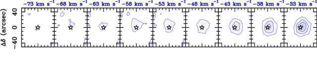
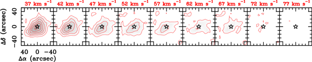
Figure 3: Velocity channel maps of the high-velocity ¹²CO (7–6) emission toward the Orion IRc2 (the star) with an effective angular resolution of 13″ (see text). Each channel map is averaged over a 5.0 km s^-1 bin whose central LSR-velocity is shown on the top of each panel. All the contours are 2$\sigma$ intervals, increasing from the 3$\sigma$ level where 1$\sigma$ is 11 K in $T_{\rm mb}$.

Figure 3 shows velocity channel maps of the HV emission. To produce the channel maps, we convolved the data with a Gaussian beam so that the effective beam size ($\theta_{\rm eff}$) becomes 13″, to obtain a higher signal-to-noise ratio (S/N). Here, the choice of 13″ is to compare with the previous work by Wilson et al. (2001), who used the HHT 10-meter telescope. The channel maps show that the redshifted gas is elongated to the (south)east of the central star, whereas the blueshifted gas seems to be distributed westward.

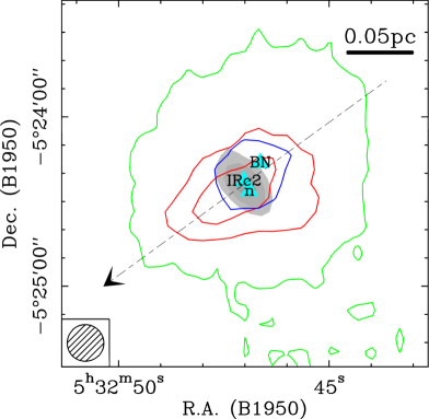
Figure 4: Comparison of the blue- and redshifted ¹²CO (7–6) high-velocity (HV) wing emission. The green contour, taken from Figure 2, represents the 50 % level contour of the CO bulk emission, and the greyscale shows the 350 $\mu$m continuum emission (Lis et al., 1998). The contours for the HV emission are 2$\sigma$ intervals, increasing from the $4\sigma$ level where $\sigma=$ 10.6 and 9.9 K$\cdot$ kms for the blue- and redshifted wings, respectively. The blue- and redshifted emission are integrated over the velocity ranges of $-75.5\leq$$V_{\rm LSR}$/km s^-1$\leq-30.5$, and $+34.5\leq$$V_{\rm LSR}$/km s^-1$\leq+79.5$, respectively (see the horizontal color-coded bars in Figure 1). The hatched circle at the bottom-right corner indicates the effective beam size ($\theta_{\rm eff}$) of 13″. The dashed line indicates the cut axis for the position-velocity diagram shown in Figure 5. The other symbols are the same as those in Figure 2. Notice that the possible heating sources discussed by de Vicente et al. (2002) are located within a region of $\sim$1$\farcs$5 radius, whose spatial-scale is almost comparable with the blue-triangle representing the IRc2 position.

The distribution of the blue- and redshifted HV wing emission is compared in Figure 4 by overlaying the integrated intensity maps. Clearly, the HV gas is confined to the innermost region of the core, inside the 50% level contour of the low-velocity bulk emission. Here, we integrated the HV emission over the velocity ranges shown in Figure 1, i.e., over the velocity range between the boundary velocity ($V_{\rm b}$), which divides the LSR-velocity range of the outflowing gas from the bulk emission, and the first highest LSR-velocity where the wing drops below the 5$\sigma$ level. We refer to such an LSR-velocity as the terminal velocity ($V_{\rm t}$). Since it is almost impossible to separate low-velocity outflowing gas from the bulk ambient gas, we arbitrarily estimated $V_{\rm b}$ from Figures 1 and 3. The redshifted gas shows an extended structure along the east-west direction, whereas the blueshifted emission arises from a compact condensation, rather than an elongated structure. It appears that the distribution of the blue- and redshifted gas is symmetric with respect to the peak position of the 350 $\mu$m continuum source, although the blue- and redshifted gas overlap each other. We prefer to interpret this as representing the pair of molecular outflow lobes previously reported [Chernin & Wright (1996); Rodríguez-Franco et al. (1999); de Vicente et al. (2002); Beuther & Nissen (2008)]. This is because their terminal velocities are too high to be interpreted in the context of the other scenarios, such as rotation or/and infall. Given its position, we exclude the BN object as a candidate source for the outflow. However, due to the limited angular resolution, our data do not give further constraints on identifying the driving source, as discussed by e.g., de Vicente et al. (2002), Beuther & Nissen (2008), Rodríguez et al. (2009), and others. Assuming that the position of IRc2 represents the center of the outflow, we made a position-velocity (PV) diagram of the CO (7–6) emission along the outflow axis (Figure 5). The PV diagram principally confirms our findings described above. Unfortunately, the CSO beam is too large to provide more detailed information about, e.g., driving mechanisms for outflow and/or outflow history.

Subsequently, we estimated the outflow lobe mass ($M_{\rm lobe}$) to calculate kinematical properties such as mass-loss rate ($\dot{M}_{\rm flow}$) and momentum rate ($F_{\rm co}$). Here, we assumed that the HV gas is optically thin and in LTE because neither isotope line, i.e., ¹³CO $J=7-6$, nor similar high-$J$ lines, e.g., ¹²CO $J=6-5$, are available with the 10″ beam. We obtained $M_{\rm lobe}$ $=$ $(1.3\pm 0.3)$ and $(3.5\pm 0.9)$ $M_{\odot}$ for the blue and red lobes, respectively, by obtaining a mean column density over the lobes of $(9.0\pm 2.4)\times 10^{17}$ and $(1.0\pm 0.3)\times 10^{18}$ cm^-2. Here, we adopted an excitation temperature ($T_{\rm ex}$) of 150 K (Comito et al., 2005), and used a ¹²CO/H₂ abundance ratio of $10^{-4}$ (Dickman, 1978). For comparison with previous publications, we adopted $d=\,450$ pc, although recent astrometry using the VLBI technique has revised the distance to the region (414$\pm$7 pc, Menten et al. 2007; 437$\pm$19 pc, Hirota et al. 2007). It is likely that the outflow masses are underestimated because of the uncertainty in defining $V_{\rm b}$. Since the highest outflow velocity is given by $\mbox{$V_{\rm flow}$}=|V_{\rm t}-V_{\rm sys}|$, the dynamical time scale ($t_{\rm d}$) is estimated from $l_{\rm lobe}$/$V_{\rm flow}$, where the lobe length $l_{\rm lobe}$ is defined as the maximum extent of the lobe measured from the IRc2 position. We assumed that the outflow inclination angle ($i$) is 45^∘, here defined as the angle between the outflow axis and the line of sight. The estimated $t_{\rm d}$ $\sim$ 900 years suggests that the outflow is extremely young. Hereafter, we describe the mean values of the outflow properties, because the derived outflow properties for the blue- and redshifted lobes are comparable within the errors. We can estimate the outflow mass-loss rate from $M_{\rm lobe}$/$t_{\rm d}$. This is $\sim 4\times 10^{-3}$ $M_{\odot}$ yr^-1 for both lobes. Since molecular outflows appear to be momentum-driven (Cabrit & Bertout, 1992), the momentum rate $F_{\rm co}$=$M_{\rm lobe}$$V_{\rm flow}^{2}$/$l_{\rm lobe}$ may be taken as an indicator of the outflow strength and hence of the mass and luminosity of the young stellar object (YSO) powering it. The outflow lobe has $\mbox{$F_{\rm co}$}\simeq 0.3$ $M_{\odot}$ km s^-1 year^-1. The derived properties are not affected significantly if one takes into account the unknown inclination angle $i$, which is defined as the angle between the outflow axis and line of sight. In fact, $t_{\rm d}$, $\dot{M}_{\rm flow}$, and $F_{\rm co}$ are corrected with factors of $\cot i$, $\tan i$, and $\sin i/\cos^{2}i$, respectively (see e.g., Davis et al. 1997). Thus, even if we assume extreme values of $i\sim 20\arcdeg$ and $70\arcdeg$, the corrections for the three quantities above would only be a factor of 3–5, thus leaving our estimates unaffected. All the derived outflow parameters are extraordinarily large, implying that the powering YSO has a bolometric luminosity of $\sim 10^{5}-10^{6}$ $L_{\odot}$, if we apply the empirical relationship between the two quantities (see Figure 5 of Richer et al. 2000 and Figure 4 of Beuther et al. 2002).

Our estimate of $\dot{M}_{\rm flow}$ to be on the order of $10^{-3}$ $M_{\odot}$ yr^-1 strongly suggests that the central massive YSO is gaining mass toward its final stellar mass through a disk-outflow system. We do not exclude the possibility that mass accretion onto the central star (or/and disk system) is currently enhanced. A statistical study of molecular outflows in 26 high-mass star-forming regions by Beuther et al. (2002) suggests that the ratio between the jet mass-loss rate and mass-accretion rate ($\dot{M}_{\rm acc}$) may be $\sim 0.2$. If this is the case, the accretion rate onto the outflow powering source would be on the order of $\sim 10^{-2}$$M_{\odot}$ yr^-1. Although the driving source of the Orion outflow has not been firmly identified, and has been a matter of debate (de Vicente et al. 2002; Beuther and Nissen 2008; Rodríguez et al. 2009), it is tempting to suggest that this accretion rate does not contradict that estimated by Nakano et al. (2000), who proposed that the central massive YSO in Orion IRc2 is either a protostar with a stellar radius of $R_{\ast}\mathrel{\hbox{\hbox to0.0pt{\hbox{\lower 4.0pt\hbox{$\sim$}}\hss}\hbox{$>$}}}300$ $R_{\odot}$ or a protostar which has a disk with $\dot{M}_{\rm acc}\approx 10^{-2}$ $M_{\odot}$ yr^-1. Nakano et al. (2000) used a one-zone model to account for the observational results of $R_{\ast}\mathrel{\hbox{\hbox to0.0pt{\hbox{\lower 4.0pt\hbox{$\sim$}}\hss}\hbox{$>$}}}300$ $R_{\odot}$ and an effective temperature of $T_{\rm eff}$$\sim$ 3000 – 5500 K (Morino et al., 1998); they adopted the latter interpretation because their model could not reproduce an $L_{\rm bol}$ $\mathrel{\hbox{\hbox to0.0pt{\hbox{\lower 4.0pt\hbox{$\sim$}}\hss}\hbox{$>$}}}4\times 10^{4}$ $L_{\odot}$ (proto)star (Kaufman et al. 1998; Gezari et al. 1998) using the low $T_{\rm eff}$ and a stellar radius larger than 30 $R_{\odot}$. More stringent calculations recently performed by Hosokawa & Omukai (2009) considered the possibility that such a massive protostar can be formed if $\dot{M}_{\rm acc}$ is higher than $4\times 10^{-3}$ $M_{\odot}$ yr^-1. If this is the case, the Keplerian speed at the protostellar surface ($v_{\rm kep}=\sqrt{GM_{\ast}/R_{\ast}}$), which is believed to represent the jet velocity (e.g., Richer et al. 2000; Arce et al. 2007), becomes $\sim 220$ km s^-1 for a 25 $M_{\odot}$ and 100 $R_{\odot}$ star. Here, the stellar mass and radius are taken from Hosokawa & Omukai (2009). We believe that our result of $V_{\rm flow}$ $\sim$ 80 – 90 km s^-1 agrees with the picture of Orion IRc2 so far obtained, especially when we consider that molecular outflows are made of ambient material entrained by a jet/winds from the central star. In conclusion, our sensitive and high-fidelity ¹²CO (7–6) line imaging demonstrates that a massive YSO is driving an extraordinarily powerful molecular outflow, suggestive of a large accretion rate. Clearly, higher resolution and better sensitivity imaging of the submm transition, as well as identification of its driving source, are required to study the spatial structure of the outflow. It may retain a history of the outflow events, a clue to understanding the mass accretion history.

References

- Arce et al. (2007) Arce, H. G., Shepherd, D., Gueth, F., Lee, C.-F., Bachiller, R., Rosen, A., & Beuther, H. 2007, Protostars and Planets V, 245
- Beuther et al. (2002) Beuther, H., Schilke, P., Sridharan, T. K., Menten, K. M., Walmsley, C. M., & Wyrowski, F. 2002, A&A, 383, 892
- Beuther & Nissen (2008) Beuther, H., & Nissen, H. D. 2008, ApJ, 679, L121
- Cabrit & Bertout (1992) Cabrit, S., & Bertout, C. 1992, A&A, 261, 274
- Chernin & Wright (1996) Chernin, L. M., & Wright, M. C. H. 1996, ApJ, 467, 676
- Comito et al. (2005) Comito, C., Schilke, P., Phillips, T. G., Lis, D. C., Motte, F., & Mehringer, D. 2005, ApJS, 156, 127
- Davis et al. (1997) Davis, C. J., Eisloeffel, J., Ray, T. P., & Jenness, T. 1997, A&A, 324, 1013
- de Vicente et al. (2002) de Vicente, P., Martín-Pintado, J., Neri, R., & Rodríguez-Franco, A. 2002, ApJ, 574, L163
- Dickman (1978) Dickman, R. L. 1978, ApJS, 37, 407
- Emerson & Graeve (1988) Emerson, D. T., & Graeve, R. 1988, A&A, 190, 353
- Gezari (1992) Gezari, D. Y. 1992, ApJ, 396, L43
- Gezari et al. (1998) Gezari, D. Y., Backman, D. E., & Werner, M. W. 1998, ApJ, 509, 283
- Hirota et al. (2007) Hirota, T., et al. 2007, PASJ, 59, 897
- Hosokawa & Omukai (2009) Hosokawa, T., & Omukai, K. 2009, ApJ, 691, 823
- Kaufman et al. (1998) Kaufman, M. J., Hollenbach, D. J., & Tielens, A. G. G. M. 1998, ApJ, 497, 276
- Kooi et al. (2000) Kooi, J., et al. 2000, Int. J. Infrared Millimeter Waves, 21, 689
- Lis et al. (1998) Lis, D. C., Serabyn, E., Keene, J., Dowell, C. D., Benford, D. J., Phillips, T. G., Hunter, T. R., & Wang, N. 1998, ApJ, 509, 299
- Marrone et al. (2004) Marrone, D. P., et al. 2004, ApJ, 612, 940
- Menten & Reid (1995) Menten, K. M., & Reid, M. J. 1995, ApJ, 445, L157
- Menten et al. (2007) Menten, K. M., Reid, M. J., Forbrich, J., & Brunthaler, A. 2007, A&A, 474, 515
- Morino et al. (1998) Morino, J.-I., Yamashita, T., Hasegawa, T., & Nakano, T. 1998, Nature, 393, 340
- Nakano et al. (2000) Nakano, T., Hasegawa, T., Morino, J.-I., & Yamashita, T. 2000, ApJ, 534, 976
- Richer et al. (2000) Richer, J. S., Shepherd, D. S., Cabrit, S., Bachiller, R., & Churchwell, E. 2000, Protostars and Planets IV, 867
- Rodríguez et al. (2009) Rodríguez, L. F., Zapata, L. A., & Ho, P. T. P. 2009, ApJ, 692, 162
- Rodríguez-Franco et al. (1999) Rodríguez-Franco, A., Martín-Pintado, J., & Wilson, T. L. 1999, A&A, 344, L57
- Sawada et al. (2008) Sawada, T., et al. 2008, PASJ, 60, 445
- Wilson et al. (2001) Wilson, T. L., Muders, D., Kramer, C., & Henkel, C. 2001, ApJ, 557, 240