Abelian deterministic self organized criticality model: Complex dynamics of avalanche waves.

Abstract

The aim of this study is to investigate a wave dynamics and size scaling of avalanches which were created by the mathematical model [J. Černák, Phys. Rev. E 65, 046141 (2002)]. Numerical simulations were carried out on a two dimensional lattice $L\times L$ in which two constant thresholds $E_{c}^{I}=4$ and $E_{c}^{II}>E_{c}^{I}$ were randomly distributed. A density of sites $c$ with the threshold $E_{c}^{II}$ and threshold $E_{c}^{II}$ are parameters of the model. I have determined autocorrelations of avalanche size waves, Hurst exponents, avalanche structures and avalanche size moments for several densities $c$ and thresholds $E_{c}^{II}$. I found correlated avalanche size waves and multifractal scaling of avalanche sizes not only for specific conditions, densities $c=0.0$, $1.0$ and thresholds $8\leq E_{c}^{II}\leq 32$, in which relaxation rules were precisely balanced, but also for more general conditions, densities $0.0<c<1.0$ and thresholds $8\leq E_{c}^{II}\leq 32$, in which relaxation rules were unbalanced. The results suggest that the hypothesis of a precise relaxation balance could be a specific case of a more general rule.

I Introduction

Bak, Tang, and Wiesenfeld (BTW) BTW introduced a concept of self-organized criticality (SOC) to study dynamical systems with spatial degree of freedom. They proposed a simple model with conservative and deterministic relaxation rules to demonstrate the SOC phenomenon. Manna Manna designed another conservative SOC model in which stochastic relaxation rules were defined. Striving to find common features of the models and to know their basic behaviors stimulated many numerical and theoretical studies during the past two decades.

Based on renormalization group calculations, Pietronero et al. Pietro claimed that both deterministic BTW and stochastic models Manna belong to the same universality class, i.e. a small modification in the relaxation rules cannot change universality class. Chessa et al. Stanley assumed that finite size scaling (FSS) is common property of both deterministic BTW and stochastic Manna models. With FSS the avalanche size, area, lifetime, and perimeter follow power laws with cutoffs Stanley :

$$P(x)=x^{-\tau_{x}}F(x/L^{D_{x}}),$$ (1)

where $P(x)$ is the probability density function of $x$, $F$ is the cutoff function, and $\tau_{x}$ and $D_{x}$ are the scaling exponents. The set of scaling exponents $(\tau_{x},\>D_{x})$ defines the universality class Stanley . A SOC model is Abelian if a final stable configuration (see below) does not depend on the relaxation order. The BTW model is Abelian, however the M model is also Abelian Dhar only if we consider probabilities of many stable configurations.

Based on numerical simulations and an extended set of exponents, Ben-Hur and Biham Hur claimed that the BTW and M models cannot belong to the same universality class. A precise numerical analysis of probability density functions $P(x)$ led Lübeck and Usadel Lubeck to the same conclusion. Essential progress to understand the discrepancy between theoretical Pietro ; Stanley and numerical conclusions Hur ; Lubeck has been achieved by Tebaldi et al. Tebaldi . They found that avalanche size probability density functions $P(s)$ do not display FSS but show a multifractal scaling i.e. the avalanche size exponent $\tau_{s}$ (Eq. 1) does not apply to the BTW model. Karmakar et al. Karmakar_prl proposed a hypothesis that the presence or absence of a precise relaxation balance between the amount released by a site and the total quantity which the same site receives when all its neighbors relax at once determines the appropriate universality class. Based on the precise relaxation balance hypothesis Karmakar_prl Karmakar and Manna Karmakar_pre proposed a flow chart to classify different SOC models into two universality classes i.e. the BTW and Manna universality classes.

The probability density functions of avalanche sizes $P(s)$ in Eq. 1 show transitions from multifractal to FSS scaling for certain densities of disturbing sites Karmakar_prl ; Cernak_2006 . The models Karmakar_prl ; Cernak_2006 are stochastic and non-Abelian with unbalanced relaxation rules Karmakar_prl . In this study, I focus on verifying an existence of such transitions for the deterministic and Abelian model cer_2002 (In the orginal paper cer_2002 the model was incorrectly clasified as non-Abelian) with unbalanced relaxation rules. The model cer_2002 displays an anomalous increase of the avalanche size area exponents $\tau_{a}$ (Eq. 1) for densities near $c=0.01$ and thresholds $E_{c}^{II}\geq 16$. However, the cause of this anomalous behavior is not well understood. I assumed that the transition from multifractal to FSS scaling could take place for density $c<0.01$ and threshold $E_{c}^{II}\geq 16$, because relaxation rules change character from balanced ($c=0.0$) to unbalanced ($c>0.0$). To characterize avalanche size scaling I investigated avalanche wave dynamics Menech ; Stella , Hurst exponents Menech , avalanche structures Hur and avalanche size moments Menech .

The paper is organized as follows. In Sec. II I repeat a definition of the inhomogeneous sand pile model cer_2002 . In Sec. III I determine autocorrelations and fluctuations of avalanche size waves, avalanche structures and avalanche size moments for several densities $0.0\leq c$$\leq 1.0$ and thresholds $8\leq E_{c}^{II}\leq 32$. Sec. IV is devoted to a discussion which is followed by conclusions in Sec. V.

II An Abelian deterministic and conservative self organized criticality model

The inhomogeneous sand pile model cer_2002 is defined on a two dimensional lattice of size $L\times L$. Each site $\mathbf{i}$ has assigned variables $E(\mathbf{i})$ and $E_{c}(\mathbf{i})$. The variable $E(\mathbf{i})$ is dynamical and it represents a physical quantity such as energy, grain density, and etc. The threshold $E_{c}(\mathbf{i})$ is a static value at site $\mathbf{i}$ which is defined only once during initialization of simulations. The threshold $E_{c}(\mathbf{i})$ has two values cer_2002 :

$$E_{c}(\mathbf{i}) = \begin{cases}E_{c}^{I}=2d\\ E_{c}^{II}=2dk,&k=2,3,4,\ldots,\end{cases}$$ (2)

where $d$ is a dimension and $k$ is a natural number. The model has two parameters namely the density $c=n/L^{2}$ and threshold $E_{c}^{II}$ where $n$ is a number of sites with the threshold $E_{c}(\mathbf{i})=E_{c}^{II}$, remaining $L^{2}-n$ sites have the threshold $E_{c}^{I}=4$. During initializations of simulations, $n$ sites with thresholds $E_{c}(\mathbf{i})=E_{c}^{II}$ were picked out randomly and all remaining sites had the threshold $E_{c}^{II}=4$, thus a set of the thresholds $\left\{E_{c}(\mathbf{i})\right\}$ represents a quenched disorder. A stable configuration is defined by a condition $E(\mathbf{i})<E_{c}(\mathbf{i})$ for each site $\mathbf{i}$. Let us assume that from a stable configuration we iteratively select $\mathbf{i}$ at random and increase $E(\mathbf{i})$$\rightarrow E(\mathbf{i})+1$. If an unstable configuration is reached i.e. $E(\mathbf{i})\geq E_{c}(\mathbf{i})$ then a relaxation starts. The relaxation rules are conservative and deterministic cer_2002 :

$$E(\mathbf{i})\rightarrow E(\mathbf{i})-\sum_{e}\triangle E(\mathbf{e}),$$ (3)

$$E(\mathbf{i}+\mathbf{e})\rightarrow E(\mathbf{i}+\mathbf{e})+\triangle E(\mathbf{e}),$$ (4)

$$\sum_{e}\triangle E(\mathbf{e})=E_{c}(\mathbf{i}),$$ (5)

where $\mathbf{e}$ is a set of vectors from the site $\mathbf{i}$ to its neighbors. The relaxation rules (Eqs. 3-5) are repeated until the site $\mathbf{i}$ becomes stable. If the neighbors of the site $\mathbf{i}$ become unstable then avalanche can run on. All unstable sites belong to the avalanche. The relaxations given by Eqs. 3-5 are repeated until a stable configuration is reached, i.e. $E(\mathbf{i})<E_{c}(\mathbf{i})$ for all sites $\mathbf{i}$. Stable and unstable configurations are repeated many times. A total number of relaxations during one avalanche is an avalanche size $s.$

III Numerical results

Numerical simulations were carried out on two dimensional lattices $L\times L$ where the linear lattice size $L$ was $L=128,\>256,\>512,\>1024,\>2048,$ and $4096$. A density $c$ and thresholds $E_{c}^{I}=4$, $E_{c}^{II}=8,\>16$ and $32$ were chosen based on the previous results cer_2002 to cover a parameter space in which interesting behaviors were expected (Sec. I). For example, near the density $c=0.01$ an anomalous increase of the avalanche area scaling exponent $\tau_{a}$ (Eq. 1) has been observed cer_2002 . Near densities $c=0.0$ and $1.0$ local relaxation rules change character from balanced ($c=0.0$ and $1.0$) to unbalanced ($c>0.0$ and $c<1.0$) Karmakar_prl ; Karmakar_pre , thus a transition from multifractal to finite size scaling could take place in the intervals $c>0.0$ and $c<1.0$. Considering these assumptions, I have selected the density $c$ as follows: $c=a$ (surroundings of $c=0.0$) or $c=1.0-a$ (surroundings of $c=1.0$) where $a=0,\>0.001,\>0.002,\>0.004,\;0.008,\;0.01,\>0.02,\>0.04,$ and $0.08$. In addition, to cover the whole interval $0.0<c<1.0$, I added the sample concentrations $c=l/10$, where $l=1,\>2,\ldots,\;9$. I have recorded about $10^{6}$ avalanches after initializations of simulations in which an avalanche dynamics has to reach the SOC state BTW . To qualify a reproducibility of the results all numerical simulations were repeated once for each lattice size $L\times L$, concentration $0.0\leq c$$\leq 1.0$ and threshold $E_{c}^{II}$. A comparison of these data sets showed that the results are well reproducible.

A possibility to decompose an avalanche into waves Ivash is a significant advantage of computer models. Because avalanche wave dynamics Menech ; Stella can provide valuable initial information about the character of an SOC model. An avalanche of size $s$ is decomposed into $m$ waves with size $s_{k}$, where $s=\sum_{k=1}^{m}s_{k}$. A time sequence of avalanche waves $s_{k}$ is used to determine the autocorrelation function Menech ; Stella

$$C(t,\>L)=\frac{\langle s_{k+t}s_{k}\rangle_{L}-\langle s_{k}\rangle_{L}^{2}}{\langle s_{k}^{2}\rangle_{L}-\langle s_{k}\rangle_{L}^{2}},$$ (6)

where time is $t=1,\>2,\ldots,$ and the time averages are taken over $5\times 10^{6}$ waves. Autocorrelations $C(t,\>L,\>c)$ have been analyzed for the time $1\leq t\leq 1000$, lattice sizes $128\leq L\leq 4096$, selected concentrations $0.0\leq c\leq 1.0$ and thresholds $E_{c}^{I}=4,$ $E_{c}^{II}=8,\>16$, and $32$ (see above). The autocorrelations $C(t,\>L=4096,\>c)$ for the biggest lattice size $L=4096$ are shown in Fig. 1. I have observed that for the density $c=1.0$, the autocorrelations $C(t,\>L=4096,\>c=1.0)$ agree within experimental error with autocorrelations of the BTW model Menech ($C(t,\>L=4096,\>c=0.0)$) . I note that the autocorrelations $C(t,\>L=4096,\>c=0.0)$ are not shown in Fig. 1. I have approximated the autocorrelations $C(t,\>L,\>c=0,\>1.0)$ by a simple function $C(t,L,c=0,\>1.0)\sim\exp(-\alpha t)$ where $\alpha$ is a decay rate cer_2008 . For more general conditions, densities $0.0<c<1.0$ (Fig. 1), the autocorrelations $C(t,\>L,\>c)$ are more complex functions than for specific densities $c=0.0$ and $1.0$. I have found that with increasing time $t$, the autocorrelations $C(t,\>L,\>c)$ are decreasing functions. An unexpected finding is the existence of oscillating components of autocorrelations. For all densities $0.0<c<1.0$ (Fig. 1(a)) and the threshold $E_{c}^{II}=8$ their periods are approximately constant. Amplitudes of oscillating components decrease with increasing density $c$ and time $t$. At the given time $t$ the autocorrelations $C(t,\>L,\>c)$ increase if a density $c$ increases, i.e. if $c_{2}\geq c_{1}$ then $C(t,\>L,\>c_{1})\geq C(t,\>L,\>c_{2})$. Near densities $c=0.0$ and $1.0$, the oscillating parts of $C(t,\>L,\>c)$ disappear. I have observed more complex behaviors (Fig. 1 (b) and (c)) for thresholds $E_{c}^{II}\geq 16$ than for the threshold $E_{c}^{II}=8$ ((Fig. 1 (a)). The oscillating components of $C(t,\>L,\>c)$ (Fig. 1(b)) have longer periods for densities $c<0.08$ and threshold $E_{c}^{II}=16$ than for the threshold $E_{c}^{II}=8$. However, odd periods were split for densities $c>0.08$. The same effect take place for the threshold $E_{c}^{II}=32$, but a critical density is higher $c\doteq 0.40$ (Fig. 1(c)). After splitting the oscillating components, for thresholds $E_{c}^{II}=16$ and $32$, their new periods were approximately equal to the period which has been found for the threshold $E_{c}^{II}=8$.

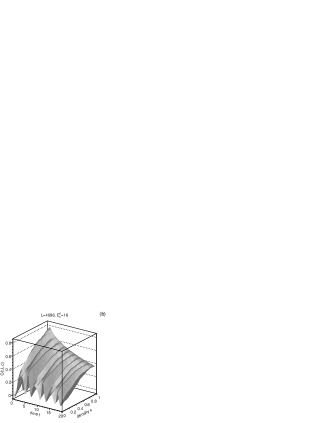
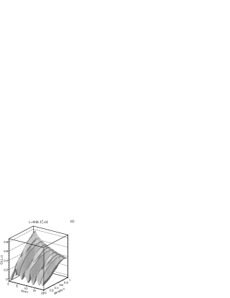
Figure 1: Autocorrelations $C(t,\>L,\>c)$ for the linear lattice size $L=4096$, for densities $0.001\leq c\leq 1.0$ and for thresholds $E_{c}^{I}=4$, (a) $E_{c}^{II}=8$, (b) $E_{c}^{II}=16$, and (c) $E_{c}^{II}=32$. The autocorrelations $C(t,L,c=0)$ are not shown.

Stochastic processes are often characterized by Hurst exponents Mandelbrot . To determine the Hurst exponent the fluctuation $F(t,\>L)$ Menech :

$$F(t,\>L)=\left[\langle\Delta y(t)^{2}\rangle_{L}-\langle\Delta y(t)\rangle_{L}^{2}\right]^{1/2}$$ (7)

is used where $y(t)=\sum_{k=1}^{t}s_{k}$ and $\Delta y(t)=y(k+t)-y(k)$. If a fluctuation $F(t,\>L)$ scales with the time $t$ as $F(t,\>L\rightarrow\infty)\sim t^{H}$ then $H$ is the Hurst exponent.

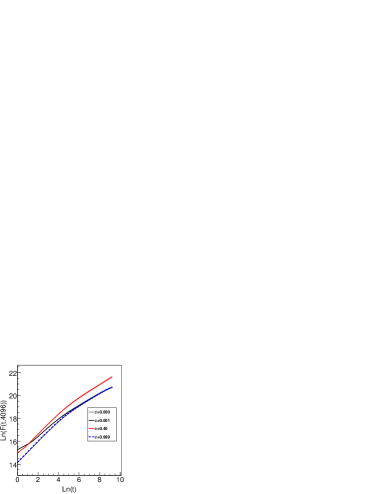
Figure 2: (Color online) Fluctuations $F(t,\>L=4096)$ for densities $c=0.000,\>0.001,\>040$ and $0.999$ and the threshold $E_{c}^{II}=32$.

I have determined fluctuations and the corresponding Hurst exponents for the lattice size $L=4096$, selected concentrations $c$ (see above) and thresholds $E_{c}^{I}=4,$ $E_{c}^{II}=8,\>16$, and $32$. For all these parameters fluctuations show two scaling regions $1<t_{1}<100$ and $1000<t_{2}<10000$. The fluctuations $F(t,\>L)$, for densities $c=0.000,\>0.001,\>040$ and $0.999$ and threshold $E_{c}^{II}=32$, are shown in Fig. 2 to demonstrate the existence of two scaling intervals. The Hurst exponents $H_{1}(c)$ and $H_{2}(c)$ as functions of density $c$ and threshold $E_{C}^{II}$ are shown for all parameters (densities $0.0\leq c\leq 1.0$ and thresholds $8\leq E_{c}^{II}\leq 32$) in Fig. 3. I have observed that the exponents $H_{1}(c)$ and $H_{2}(c)$ depend on the parameters (density $c$ and threshold $E_{C}^{II}$) in a nontrivial manner (Fig. 3). For densities $0.0\leq c\leq 1.0$ and thresholds $8\leq E\leq 32$ functions $H_{1}(c)$ are bounded by the interval $0.68<H_{1}(c)<0.81$. Similarly, the functions $H_{2}(c)$ are limited by the interval $0.44<H_{2}(c)\leq 0.56$. The exponents $H_{1}(c)\doteq 0.80$ and $H_{2}(c)\doteq 0.50$ are approximately constant for densities $c>0.50$. I have observed anomalous decreases of functions $H_{1,\,2}(c)$ near low densities $0.0<c\leq 0.01$ (Fig. 3). In addition, functions of $H_{1\,,2}(c)$ have a decreasing tendency if the second thresholds $E_{c}^{II}$ increase. Finally, the functions $H_{1,2}(c)$ are not symmetric around the density $c=1/2$, i.e. $H_{1}(0.5-a)\neq H_{1}(0.5+a)$ and $H_{2}(0.5-a)\neq H_{2}(0.5+a)$ for $0.0<a<0.5$ except the specific densities $c=0.0$ and $c=1.0$, where $H_{1}(0.0)\doteq H_{1}(1.0)$ and $H_{2}(0.0)\doteq H_{2}(1.0)$ within experimental errors.

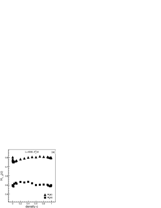
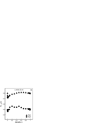
Figure 3: Hurst exponents $H_{1}(c)$and $H_{2}(c)$ as functions of a densities $c$ and thresholds: $E_{c}^{I}=4$, (a) $E_{c}^{II}=8$, (b) $E_{c}^{II}=16$, and (c) $E_{c}^{II}=32$ for the lattice size $4096\times 4096$. The Hurst exponents at given density $c$, $H_{1}(c)$ and $H_{2}(c)$ were approximated using the power laws $F(t,\>L)\sim t^{H_{1}(c)}$ and $F(t,\>L)\sim t^{H_{2}(c)}$ in the intervals $t=1-100$ and $t=10^{3}-10^{4}$.

Ben-Hur and Biham Hur proposed to use avalanche structures to demonstrate a difference between BTW BTW and M Manna models. An avalanche structure consists of clusters of sites with equal numbers of relaxations. The BTW model displays rigorous shell-like structures Hur ; Karmakar_prl and the M model displays disordered structures Hur with inner holes Karmakar_prl . I have analyzed several avalanche structures (Fig. 4) of the inhomogeneous sand pile model cer_2002 to compare them with known structures Hur ; Karmakar_prl .

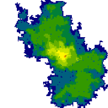
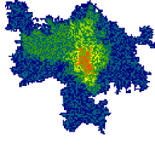
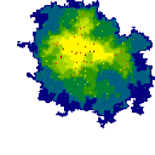
(a) (b) (c)

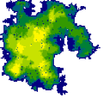
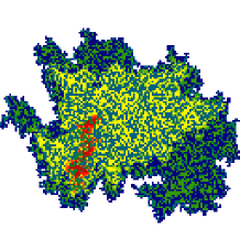
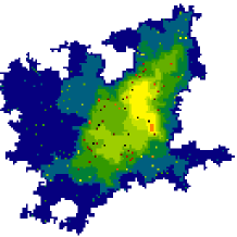
(d) (e) (f)

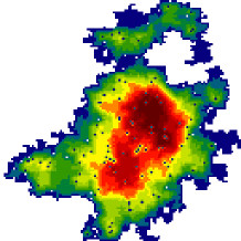
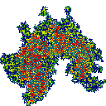
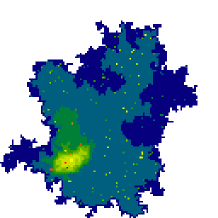
(g) (h) (i)

Figure 4: Avalanche structures on two dimensional lattice $128\times 128$ for parameters $E_{c}^{I}=4$, (a) $E_{C}^{II}=8$, $c=0.02$, (b) $E_{C}^{II}=8$, $c=0.5$, (c) $E_{C}^{II}=8$, $c=0.98$, (d) $E_{C}^{II}=16$, $c=0.02$, (e) $E_{C}^{II}=16$, $c=0.5$, (f) $E_{C}^{II}=16$, $c=0.98$, (g) $E_{C}^{II}=32$, $c=0.02$, (h) $E_{C}^{II}=32$, $c=0.5$, and (i) $E_{C}^{II}=32$, $c=0.98$. Lattice sites with the same numbers of relaxations are shown by the same color (rainbow pseudo-color coding).

I have observed the avalanche structures which resemble the shell-like structure for densities $c=0.02$ (Fig. 4(a), (d), and (g)) and $c=0.98$ (Fig. 4 (c), (f), and (i)). However, these structures are not exactly shell-like. A clear visible difference is the existence of holes in an avalanche, for example see Figs. 4(a), (b), and (d). The sizes of these holes vary from one site (obviously a site with $E_{c}^{II}>E_{c}^{I}$) to several sites. Mainly, for low densities ($c=0.02)$ an existence of holes is clearly demonstrated in Figs. 4(a), (d), and (g) where the sites with the threshold $E_{c}^{II}$ can absorb and relax more energy than surrounding sites with $E_{c}^{I}$. If the sites ($E_{c}^{II}$) absorb energy then they are well identified as small holes inside the avalanche structure (Figs. 4(a), (d), and (g)). If the sites ($E_{c}^{II}$) release more energy than their neighbors (with threshold $E_{c}^{I}$) then the sites ($E_{c}^{II}$) involve instabilities of many sites within a certain distance. These sites must relax to be stable (Fig. 4 (d)). At high density $c=0.98$, the sites with the lower threshold $E_{c}^{I}$ are considered for disturbing sites. A site with threshold $E_{c}^{I}$ can receive more energy from neighbors than a critical amount of the site (threshold $E_{c}^{I}$). Then the site ($E_{c}^{I}$) must relax more times than neighbors (sites with the threshold $E_{c}^{II}$) to be stable. The disturbing sites are shown as isolated sites in Figs. 4(c), (f), and (i). The effects of disturbing sites $E_{c}^{II}$ and $E_{c}^{I}$ differs, for the small density $c=0.02$, the disturbing sites $E_{c}^{II}$ can absorb and relax more energy as their neighbors. However, for high density $c=0.98$, the disturbing sites $E_{c}^{I}$ can only do more relaxations than their neighbors sites.

I have found new avalanche structures which resemble neither shell-like (the BTW mode) nor disordered (the M model) Hur ; Karmakar_prl for density $c=0.50$ and thresholds $8\leq E_{c}^{II}\leq 32$ Figs. 4(b), (e), and (h). Their typical feature is the existence of complex clusters in avalanche which more resemble percolation clusters.

The model (Sec. II) displays shell-like avalanche structures as well as the BTW model Hur ; Karmakar_prl only for the specific densities $c=0.0$ and $c=1.0$.

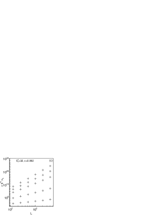
Figure 5: Scaling of avalanche size moments $\langle s^{q}\rangle$ versus the lattice size $128\leq L\leq 4096$. The exponents $q$ are $q=1.0,\>2.0,\>3.0,\>3.5$ and $3.95$ from bottom to top. The model parameters are $E_{c}^{I}=4$, $E_{c}^{II}=32$, (a) $c=0.008$, (b) $c=0.40$ and (c) $c=0.992$.

Sometimes we cannot decompose an avalanche into waves, obviously if we study real systems, then avalanche moments Menech are useful. A property $x$ in FSS obeys scaling given by Eq. 1. The moments $q$ are Menech :

$$\langle x^{q}\rangle=\int_{{}_{0}}^{x_{max}}x^{q}P(x,L)dx\sim L^{\sigma_{x}(q)}$$ (8)

where $\sigma_{x}(q)=(q+1-\tau_{x})D_{x}$ and $x_{max}\sim L^{D_{x}}$. I have determined only avalanche size moments $\langle s^{q}\rangle$ versus the lattice size $L$ which are shown in Fig. 5 for densities $c=0.008$, $c=0.40$ and $c=0.992$ and for thresholds $E_{c}^{I}=4$ and $E_{c}^{II}=32$. The moments $\langle s^{q}\rangle$ scale with the lattice size $L$ as well as $\langle s^{q}\rangle\sim L^{\sigma_{x}(q)}$ (Eq. 8), thus a basic requirement is met to determine $\sigma_{s}(q)$.

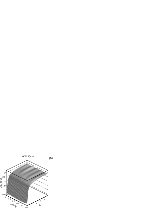
Figure 6: Plots $\partial\sigma_{s}(q)/\partial q$ versus exponent $q$ for the lattice size $4096\times 4096$, concentrations $0.0<c\leq 1.0$ and thresholds: $E_{c}^{I}=4,$ (a) $E_{c}^{II}=8$, (b) $E_{c}^{II}=16$, and (c) $E_{c}^{II}=32$.

Using the functions $\sigma_{s}(q)$ I determined the plots $\partial\sigma_{s}(q)/\partial q$ versus the exponent $q$ which are shown in Fig. 6 for densities $0.0<c\leq 1.0$ and thresholds $4<E_{c}^{II}\leq 32$. I have observed that the functions $\partial\sigma_{s}(q)/\partial q$ are increasing if exponents $q$ increase (Fig. 6) for exponents $q>1.0$, densities $0.0<c<1.0$ and thresholds $8\leq E_{c}^{II}\leq 32$. Surface cuts $\partial\sigma_{s}(q)/\partial q\>\mid_{q=1.0}$ and $\partial\sigma_{s}(q)/\partial q\>\mid_{q=4.0}$, for exponents $q=1.0$ and $q=4.0$, as functions of density $c$ are shown in Fig. 7 to demonstrate this increasing tendency. I have found that $\partial\sigma_{s}(q)/\partial q\>\mid_{q=4.0}>\partial\sigma_{s}(q)/\partial q\>\mid_{q=1.0}$, $\partial\sigma_{s}(q)/\partial q\>\mid_{q=1.0}\neq const.$ and $\partial\sigma_{s}(q)/\partial q\>\mid_{q=4.0}\neq const.$ (Fig. 7) for densities $0.0<c<1.0$ and thresholds $8\leq E_{c}^{II}\leq 32$. This implies that functions $\partial\sigma_{s}(q)/\partial q$ differ from the function $\partial\sigma_{s}(q)/\partial q$ of the BTW model. However, for the specific parameters $c=0.0$, $c=1.0$ and $8\leq E_{c}^{II}\leq 32$ relaxation rules are precisely balances and the functions $\partial\sigma_{s}(q)/\partial q$ versus $q$ ($q\geq 1.0$) are identical within experimental errors with the function $\partial\sigma_{s}(q)/\partial q$ of the BTW model Menech ; Karmakar_prl .

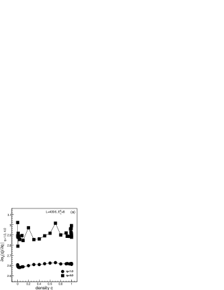
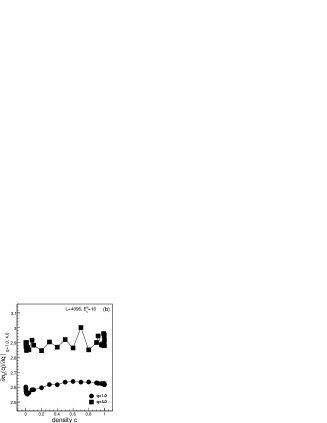
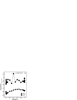
Figure 7: The plots $\partial\sigma_{s}(q)/\partial q\mid_{q=1}$ (errors $\pm 0.01$) and $\partial\sigma_{s}(q)/\partial q\mid_{q=4}$(errors $\pm 0.03$) versus density $c$ for the linear lattice size $L=4096$ and thresholds $E_{c}^{I}=4$, (a) $E_{c}^{II}=8$, (b) $E_{c}^{II}=16$, and (c) $E_{c}^{II}=32$.

IV Discussion

I have found that autocorrelations $C(t,\>L,\>c)$ (Fig. 1) are more complex functions than an autocorrelation of the BTW model Menech ; Karmakar_prl . The autocorrelations exhibit oscillating components (Fig. 1) which periods and amplitudes depend on both densities $0.0<c<1.0$ and thresholds $8\leq E_{c}^{II}\leq 32$. The oscillating components are probably caused by a periodicity in an avalanche wave sequence. I assume that the periodicity could be a consequence of an excessive energy storing and release in sites with the thresholds $E_{c}^{II}$, apparently when the sites have low concentration $c<0.5$. In such conditions, relaxations of these sites trigger relaxations of surrounding sites, i.e. all surrounding sites within a certain distance from a disturbing site have to relax cer_2002 . This hypothesis could be supported by finding that for the same time $t$ amplitudes of oscillating components are decreasing if densities $c$ increase and oscillations disappear near the density $c=1.0$ (Fig. 1). The periods were longer for low densities $c<0.4$ and thresholds $E_{c}^{II}\geq 16$ than for the threshold $E_{c}^{II}=8$. This could be connected with the stronger effect of disturbing sites $E_{c}^{II}\geq 16$ which can store and release much more energy than disturbing sites $E_{c}^{II}=8$. However, a nontrivial dependence of periods on thresholds $E_{c}^{II}\geq 8$ and densities $c$ (Fig. 1) and the cause of period splitting for thresholds $E_{c}^{II}\geq 16$ and critical densities $c$ (Fig. 1 (b) and (c)) are not understood. For specific densities $c=0.0$ and $c=1.0$, the autocorrelations $C(t,\>L,\>c=0.0)$ and $C(t,\>L,\>c=1.0)$ agree well with autocorrelation of the BTW model Karmakar_prl ; Menech . I have found correlated avalanche waves under more general conditions in which the relaxation rules are unbalanced Karmakar_prl for densities $0.0<c<1.0$ and thresholds $8\leq E_{c}^{II}\leq 32$. This is completely opposite to the result the hypothesis predicted Karmakar_prl ; Karmakar_pre . I think that the hypothesis about a precise relaxation balance Karmakar_prl ; Karmakar_pre is valid only for the specific densities $c=0.0$ and $c=1.0$ and thresholds $8\leq E_{c}^{II}\leq 32$.

Two scaling intervals of fluctuations $F(t,\>L=4096)$ (Fig. 3) support correlated avalanche waves Menech for densities $0.0\leq c\leq 1.0$ and thresholds $8<E_{c}^{II}\leq 32$. The fluctuations $F(t,\>L=4096)$ agree well with a fluctuation of the BTW model only for the densities $c=0.0$ and $c=1.0$ Menech ; Karmakar_prl when relaxation rules are precisely balanced Karmakar_prl . For all other parameters, densities $0.0<c<1.0$ and thresholds $8\leq E_{c}^{II}\leq 32$, relaxation rules are unbalanced and the hypothesis Karmakar_prl ; Karmakar_pre predicts a single scaling region with the Hurst exponent $H=1/2$. However, I have not found single scaling regions of $F(t,\>L=4096)$. So the fluctuations $F(t,\>L=4096)$ contradict the hypothesis of precise relaxation balance Karmakar_prl ; Karmakar_pre . Asymmetries of functions $H_{1,2}(c)$ to permutations of densities $c$ (Fig. 3) could be a consequence of different local effects of disturbing sites $E_{c}^{II}$ near density $c=0.0$ and disturbing sites $E_{c}^{I}$ near density $c=1.0$. The Hurst exponents $H_{1}(c)$ are limited by the interval $0.68<H_{1}(c)<0.8$ near the density $c=0.0$ thus avalanche waves are less correlated than in the BTW model ($H_{1}=0.8$) and they are more correlated than in the M model ($H=0.5$). The Hursts exponents $H_{2}(c)$ are limited by the interval $0.44<H_{2}(c)\leq 0.56$ which indicate that local perturbation effects can change a long-term persistence (antipersistence) Mandelbrot . The changes of Hurst exponents $H_{1,2}(c)$ with density $c$ and threshold $E_{c}^{II}$ demonstrate that local perturbation effects could change a global wave dynamics.

I assume that avalanche wave dynamics (autocorrelations and fluctuations) on a finite size lattices $L\times L$, for $L>L_{c}$ where $L_{c}$ is a critical length, can provide basic information about correlated (the BTW model) or uncorrelated (the M model) nature of waves in avalanches not only for the finite size $L$ but also for the size $L$ which goes to infinity. I assume that $L=4096$ is greater than $L_{c}$. Then conclusions regarding an avalanche wave dynamics for the finite lattice size $L=4096$ could be extended for infinite systems.

A comparison of avalanche structures, for densities $0.0<c<1.0$ and thresholds $8\leq E_{c}^{II}\leq 32$, shows that the avalanche structures of the model (Sec. II) are more disordered than shell-like structures of the BTW Hur ; Karmakar_prl model but they are more ordered than structures of the M model Hur ; Karmakar_prl . Only for the specific densities $c=0.0$ and $c=1.0$, the avalanche structures are exactly shell-like as well as in the BTW model Hur ; Karmakar_prl . I assume that connection between avalanche structures and autocorrelations near the density $c=0.5$ are more weak for the model (Sec. II) than for the BTW or M models Hur ; Karmakar_prl . Because avalanche structures are more disordered (Fig. 4) than structures of the BTW model and more ordered than structures of the M model, however avalanche waves are correlated as in Fig. 1.

A hypothesis about a precise relaxation balance Karmakar_prl for unbalanced relaxation rules predicts FSS where $\partial\sigma_{s}(q)/\partial q=const.$ for all exponents $q>1.0$. In such case, an expectation $\partial\sigma_{s}(q)/\partial q\>\mid_{q=4}\doteq\partial\sigma_{s}(q)/\partial q\>\mid_{q=1}$ is correct. However, avalanche size moments do not support this expectation, because I have found that $\partial\sigma_{s}(q)/\partial q\>\mid_{q=4}>\partial\sigma_{s}(q)/\partial q\>\mid_{q=1}$ and functions $\partial\sigma_{s}(q)/\partial q\>\mid_{q=4}$ and $\partial\sigma_{s}(q)/\partial q\>\mid_{q=1}$ (Fig. 7) depend on a density $c$ for all densities $0.0<c<1.0$ and thresholds $8\leq E_{c}^{II}\leq 32$. This is a reason why functions $\partial\sigma_{s}(q)/\partial q$ of the model (Sec. II) cannot be identical with the function $\partial\sigma_{s}(q)/\partial q$ of the BTW model Karmakar_prl ; Manna ($c=0.0$ and $1.0$) for densities $0.0<c<1.0$. Although, I conclude that avalanche waves are correlated in avalanches and avalanche sizes scale as a multifractal for all investigated parameters.

For specific densities $c=0.0$ and $1.0$, the basic assumptions $H_{i}-H_{i}^{{}^{\prime}}=0$ of the precise relaxation balance hypothesis Karmakar_prl are correct. However, all results (Sec. III) show a multifractal scaling of avalanche sizes not only for the specific conditions but also for the more general conditions $0.0<c<1.0$ and $8\leq E_{c}^{II}\leq 32$ in which $|H_{i}-H_{i}^{{}^{\prime}}|=4n$, $0\leq n\leq 7$ where $n$ is a natural number. Thus I conclude that the hypothesis about precise relaxation balance Karmakar_prl is valid only for the specific parameters $c=0.0$ and $1.0$ and $E_{c}^{II}>4$.

I have not observed a transition from multifractal scaling to FSS of avalanche sizes which has been expected for low densities near $c=0.0$ (Sec. I). However, the autocorrelations, Hurst exponents and avalanche size moments support the previous conclusions cer_2002 ; cer_2008 ; Cernak_2006 that multifractal scaling is very sensitive to local perturbations for densities near $c=0.0$.

Does the model belong to the BTW class? The answer is not uniform. The model shows common features with the BTW model for example, correlated waves in avalanches and multifractal scaling of avalanche sizes. However, I have demonstrated that the autocorrelations (Fig. 1) are complex functions, Hurst exponents are functions of densities $c$ (Fig. 3) and holes can be found in avalanches while all these features are not typical for the BTW model. A possible difference between the inhomogeneous sand pile model cer_2002 and the BTW model BTW is supported by functions $\partial\sigma_{s}(q)/\partial q$ (Figs. 6 and 7) which are not identical with the function $\partial\sigma_{s}(q)/\partial q$ of the BTW model except the specific densities $c=0.0$ and $1.0$.

V Conclusion

Applying the classification scheme Karmakar_pre on the inhomogeneous sandpile model model (Sec. II) places the model in the M universality class. However, I have demonstrated (Sec. III) that the model belongs neither in the M universality class nor in the BTW universality class (Sec. IV). I assume that it belongs in a multifractal universality class Tebaldi which is more general than the BTW class cer_2008 . Based on the wave autocorrelations, fluctuations, avalanche structures and avalanche size moments, I conclude that an avalanche wave dynamics and avalanche size scaling depend on local relaxation details. In addition, a hypothesis about precise relaxation balance Karmakar_prl ; Karmakar_pre could be a specific case of a more general rule. The reason why a multifractal scaling is very sensitive to local perturbations is not well understood.

- (1) P. Bak, C. Tang, and K. Wiesenfeld, Phys. Rev. Lett. 59, 381 (1987).
- (2) S. S. Manna, J. Phys. A 24, L363 (1991).
- (3) L. Pietronero, A. Vespignani, and S. Zapperi, Phys. Rev. Lett. 72, 1690 (1994).
- (4) A. Chessa, H. E. Stanley, A. Vespignani, and S. Zapperi, Phys. Rev. E 59, R12 (1999).
- (5) Dhar, Physica A 270, 69 (1999).
- (6) A. Ben-Hur and O. Biham, Phys. Rev. E 53, R1317 (1996).
- (7) S. Lübeck and K. Usadel, Phys. Rev. E 55, 4095 (1997).
- (8) C. Tebaldi, M. De Mennech, and A. L. Stella, Phys. Rev. Lett. 83, 3952 (1999).
- (9) R. Karmakar, S. S. Manna, and A. L. Stella, Phys. Rev. Lett. 94, 088002 (2005).
- (10) R. Karmakar and S.S. Manna, Phys. Rev. E 71, 015101(R) (2005).
- (11) J. Černák, Phys. Rev. E 73, 066125 (2006).
- (12) J. Černák, Phys. Rev. E 65, 046141 (2002).
- (13) M. de Menech and A.L. Stella, Phys. Rev. E 62, R4528 (2000).
- (14) A. L. Stella and M. de Menech, Physica A 295, 101 (2001).
- (15) E. V. Ivashkevich, D.V. Ktitarev, and V. B. Priezzhev, Physica A 209, 347 (1994).
- (16) J. Černák, arXiv:0807.4113v2 [cond-mat.stat-mech].
- (17) Benoit B. Mandelbrot, The fractal geometry of nature (W. E. Freeman and Company, New York, 1983).