Ultrafast stimulated Raman parallel adiabatic passage by shaped pulses

Abstract

We present a general and versatile technique of population transfer based on parallel adiabatic passage by femtosecond shaped pulses. Their amplitude and phase are specifically designed to optimize the adiabatic passage corresponding to parallel eigenvalues at all times. We show that this technique allows the robust adiabatic population transfer in a Raman system with the total pulse area as low as 3 $\pi$, corresponding to a fluence of one order of magnitude below the conventional stimulated Raman adiabatic passage process. This process of short duration, typically pico- and subpicosecond, is easily implementable with the modern pulse shaper technology and opens the possibility of ultrafast robust population transfer with interesting applications in quantum information processing.

I Introduction

Complete or partial population transfer between ground states by pulsed laser fields is at the heart of many quantum processes Shore ranging from laser-controlled chemistry Shapiro to modern quantum optics and quantum information, such as quantum gates QI .

Standard $\pi$-pulse techniques that require a specific pulse area are known to lack robustness Allen ; Holthaus . Adiabatic passage, which allows the dynamics to follow a single eigenstate of the system, is often used to implement such transfers due to its robustness with respect to field fluctuations and to the imperfect knowledge of the studied system. In particular, the stimulated Raman adiabatic passage (STIRAP) process, which induces a complete population transfer in a $\Lambda$ system STIRAP , and various extensions Vitanov-review ; Shapiro_CC ; Adv , have become very popular. The main advantage relies on its dark-state dynamics which does not involve the upper state in the adiabatic limit, and makes thus this process in principle immune to decoherence. However this process requires in practice a large pulse area to satisfy the adiabaticity and prevents in most cases its use for pulses shorter than nanoseconds.

On the basis of the adiabatic theorem, it is commonly believed that a large pulse area for adiabatic passage is inevitable and that it is the price to pay to get the robustness. It has been however found that, for a two-level system driven by an appropriate shaped chirped pulse, the pulse area can be only typically $1.5\pi$ Parallel , which is not much larger than the $\pi$ value (corresponding to the smallest value leading to a complete population transfer for a pulse of a laser perfectly tuned to the resonance, the $\pi$-pulse OptControl ). This finding has been made from a geometric picture showing the surfaces of eigenenergies as functions of the field parameters Topology : the paths that optimize the non-adiabatic losses are level-lines in the diagram of the distance between the two surfaces and correspond to instantaneous eigenvalues that are parallel at all times.

In a $\Lambda$-system (where we assume that the two ground states are not coupled, e.g. for symmetry reasons), the naive simplest way to completely transfer the population between the two ground states is two successive $\pi$ pulses, one for each transition, leading to a total pulse area of $2\pi$. One can also consider two exactly overlapping fields also giving a total pulse area of $2\pi$ Shore . It has been shown that the minimum area for such a process is $\sqrt{3}\pi$, which corresponds to the singular-Riemannian geodesic OptControl .

We show in this paper that one can extend the optimization procedure making the dynamics follow parallel eigenvalues at all times to a $\Lambda$-system driven by two appropriately shaped fields of chirped frequencies. One gets a complete population transfer for a total pulse area as low as 3$\pi$ with the standard robustness of adiabatic processes. This opens the possibility to implement ultrafast Raman adiabatic passage technique, i.e. in the pico-and subpicosecond regime, using the state-of-the-art technology of shaped femtosecond laser pulses (see for instance Weiner ; Chatel and its recent use and proposals for strategies of control Gerber ; Silberberg ; Brixner ; Baumert ; Ultimate ).

The paper is organized as follows. We first describe the technique of parallel adiabatic passage in $\Lambda$-systems. We next compare it with respect to the conventional STIRAP. Robustness with respect to fluctuations is analyzed. Before concluding, we propose an implementation of the parallel STIRAP using pulse shaping techniques.

II Parallel adiabatic passage in $\Lambda$-systems

II.1 The system

The $\Lambda$-system, with the two ground states denoted respectively $|1\rangle$ and $|3\rangle$, driven by two fields, respectively the pump and the Stokes fields, is described in the resonant approximation Shore in the dressed-state basis by the Hamiltonian

$${\sf H}^{[\Omega_{P},\Omega_{S},\Delta,\delta]}=\frac{1}{2}\left[\begin{array}[]{ccc}0&\Omega_{P}&0\\ \Omega_{P}&2\Delta&\Omega_{S}\\ 0&\Omega_{S}&2\delta\end{array}\right].$$ (1)

The available parameters that can a priori vary during time are $\Omega_{P}$ and $\Omega_{S}$ (chosen real for simplicity) the pump and Stokes Rabi frequencies coupling the transitions $|1\rangle-|2\rangle$ and $|3\rangle-|2\rangle$ respectively, $\Delta$ and $\delta$ respectively the one-photon detuning (with respect to the pump) and the two-photon detuning: $\Delta=\omega_{2}-\omega_{1}-\omega_{P}$, $\delta=\omega_{3}-\omega_{1}-\omega_{P}+\omega_{S}$ with $\hbar\omega_{j}$, $j=1,2,3$, the energies of the corresponding state $|j\rangle$ and $\omega_{P}$, $\omega_{S}$ the frequencies of the pump and Stokes fields respectively.

II.2 Construction of parallel eigenvalues

We apply the analysis that was made in Ref Parallel for a two-state system to the three-state model: We require an adiabatic passage process such that the eigenvalues stay parallel at each time in order to optimize the adiabatic passage. We first remark that this imposes fields of chirped frequency. The use of (non-optimized) linearly chirped fields has been proposed in Band and studied in Sola with the aim of minimizing the intermediate-level population. We first determine sufficient conditions to achieve the parallelism of the eigenvalues and next give a time-dependent realization that can be implemented using modern pulse shapers.

Adiabatic passage processes require the knowledge of the eigenelements. For the case of a two-photon detuning, they have been determined and studied for instance in Fewell . Here we require the parallelism of the eigenvalues. More precisely, denoting $\omega_{-,0,+}$ the three eigenvalues satisfying at each time $\omega_{-}<\omega_{0}<\omega_{+}$ and $|\psi_{-,0,+}\rangle$ the corresponding eigenstates, we impose for reasons of symmetry $\omega_{+}-\omega_{0}=\omega_{0}-\omega_{-}$ and that $|\psi_{0}\rangle$ transports adiabatically the population, thus connecting at early times the initially populated state $|1\rangle$ and at late times the target state $|3\rangle$: $|1\rangle\buildrel t\to-\infty\over{\longleftarrow}|\psi_{0}\rangle\buildrel t\to+\infty\over{\longrightarrow}|3\rangle$. The eigenvalues are thus of the form

$$\omega_{0}=\frac{1}{3}(\Delta+\delta),\quad\omega_{\pm}=\frac{1}{3}(\Delta+\delta)\pm\frac{1}{2}\Omega_{0},$$ (2)

with

$$\Omega_{0}=\sqrt{\Omega_{P}^{2}+\Omega_{S}^{2}+\frac{4}{3}(\Delta^{2}-\Delta\delta+\delta^{2})}$$ (3)

and the condition

$$0=[9(\Omega_{P}^{2}+\Omega_{S}^{2})-4(2\Delta-\delta)(2\delta-\Delta)]\frac{\Delta+\delta}{27}-\Omega_{P}^{2}\delta.$$ (4)

The initial connection, when $\Omega_{P}=\Omega_{S}=0$, imposes for the time-dependent detuning $\delta(-\infty)=-\Delta(-\infty)=\Omega_{0}/2$ corresponding to $\omega_{0}(-\infty)=0$, and $\omega_{\pm}(-\infty)=\pm\Omega_{0}/2$. The final connection can be chosen in two ways: Either $\omega_{+}(+\infty)=0$, $\omega_{0}(+\infty)=-\Omega_{0}/2$, $\omega_{-}(+\infty)=-\Omega_{0}$, or $\omega_{+}(+\infty)=\Omega_{0}$, $\omega_{0}(+\infty)=\Omega_{0}/2$, $\omega_{-}(+\infty)=0$. We have chosen below the latter situation corresponding to $\delta(+\infty)=\Omega_{0}/2$ and $\Delta(+\infty)=\Omega_{0}$. At this stage, we expect many solutions for the four available parameters from Eqs. (3) and (4) with boundary conditions: $0\buildrel t\to-\infty\over{\longleftarrow}\Omega_{P,S}(t)\buildrel t\to+\infty\over{\longrightarrow}0$, $-\Omega_{0}/2\buildrel t\to-\infty\over{\longleftarrow}\Delta(t)\buildrel t\to+\infty\over{\longrightarrow}\Omega_{0}$, $\Omega_{0}/2\buildrel t\to-\infty\over{\longleftarrow}\delta(t)\buildrel t\to+\infty\over{\longrightarrow}\Omega_{0}/2$.

II.3 Numerical implementation

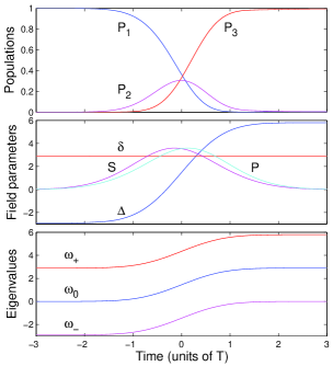
Figure 1: Transition Probability for a level line dynamics as function of time for $\Omega_{0}=5.8/T$ (corresponding to the total pulse area ${\cal A}\approx 3.6\pi$). Upper frame: Population $P_{j}=|\langle j|\phi(t)\rangle|^{2}$ with $\phi(t)$ the state solution. Middle frame: The field parameters (in units of $1/T$) $\Delta(t)$, $\delta(t)$ given by Eqs. (5) (for $\alpha=0$), and $\Omega_{P}(t)$ and $\Omega_{S}(t)$ determined from Eqs. (3) and (4). Lower frame: The eigenvalues (in units of $1/T$).

To find a simple implementable solution, we additionally impose the time parametrization as a monotonic smooth function for $\Delta(t)$, symmetric around $t=0$, and a symmetric Gaussian shape for $\delta(t)$:

$$\Delta(t)=\frac{3\Omega_{0}}{4}\text{erf}\bigl{(}\frac{t}{T}\bigr{)}+\frac{\Omega_{0}}{4},\ \delta(t)=\frac{\Omega_{0}}{2}[1+\alpha e^{-(\beta t/T)^{2}}],$$ (5)

with $\alpha$ and $\beta$ to be chosen. The quantity $T$ corresponds to a characteristic time of the duration of the process. The choice $\alpha=0$ is simple since it leads to a constant two-photon detuning; it will be shown to give already very good results. For given $\alpha$ and $\beta$, the choice $\Omega_{0}$ comes down to choose a unique level line for the problem and set the values of the Rabi frequencies $\Omega_{P}(t)$ and $\Omega_{S}(t)$ from Eqs. (3) and (4). Note that the parametrization (5) is somewhat arbitrary. Other smooth shapes for the detunings lead to very similar (but not strictly identical) results.

We define the total pulse area for the process as

$${\cal A}=\int_{-\infty}^{+\infty}dt\sqrt{\Omega_{P}^{2}(t)+\Omega_{S}^{2}(t)}.$$ (6)

This characteristic quantity is known to be at least $\pi$ when one considers a two-state transition (for instance the 1-2 transition by the pump field) OptControl . The pulse area has a clear-cut dynamical meaning only for resonant pulses in two-level systems. In other (nonresonant, multilevel) situations, different pulses with the same individual area can produce different results even in near-adiabatic cases. This choice of the total pulse area takes also into account the delay between the pulses. Considering for simplicity two identical delayed pulses of individual area ${\cal A}_{P}$, the area ${\cal A}$ is bounded between $\sqrt{2}{\cal A}_{P}$ (no delay) and $2{\cal A}_{P}$ (consecutive pulses without overlapping). This criterion favors thus overlapping pulses since they lead to faster processes. In the $\Lambda$ system, the use of two successive $\pi$ pulses, respectively for the pump and Stokes fields, or of two overlapping fields corresponds both to ${\cal A}=2\pi$ Shore . However it is known that the minimum area for such a process is $\sqrt{3}\pi$ OptControl . An alternative quantity of interest is the total fluence corresponding to an integrated intensity:

$${\cal F}=\int_{-\infty}^{+\infty}dt(\Omega_{P}^{2}(t)+\Omega_{S}^{2}(t)).$$ (7)

Figure 1 shows the resulting dynamics corresponding to parallel eigenvalues with $\Omega_{0}=5.8/T$ and $\alpha=0$. We obtain ${\cal A}\approx 3.6\pi$ and ${\cal F}\approx 40/T$ in these conditions. The obtained final population transfer $P_{3}(+\infty)\approx 0.995$ shows a very efficient population transfer by adiabatic passage for a quite modest pulse area, only approximately twice the minimum required area $\sqrt{3}\pi$. One can notice the counterintuitive sequence of the pulses (i.e. the Stokes field coming first before the pump field), which appears here as a consequence of the level line procedure for the choice (5). We notice a non-negligible transient population in the upper state 2 since here the dynamics is not governed by a dark state. We however anticipate that a fast enough process, typically subpicosecond, will allow one to neglect the resulting loss from the upper state.

III Comparison with the conventional STIRAP

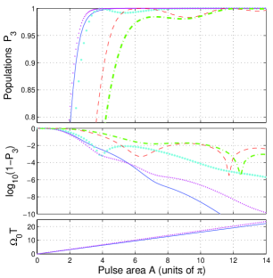
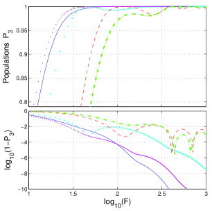
Figure 2: Upper frame: Final population transfer for the parallel STIRAP with $\alpha=0$ (full line), linearization of $\Delta(t)$ [see Eq. (10)] (large-dotted line), the conventional STIRAP with the delay $\tau=1.1T$ (dashed line) and with the delay $\tau=T$ (dot-dashed line), and parallel STIRAP with $\alpha=0.1/T$ and $\beta=1.25$ (thin-dotted line) as a function of the total pulse area ${\cal A}$. Middle frame: logarithmic scale of the deviation from the complete population transfer. Lower frame: The corresponding $\Omega_{0}T$ for the parallel STIRAP’s.

Figure 3: Same as Fig. 3 but as a function of the fluence ${\cal F}$ (in units of $1/T$) in logarithmic scale.

Figures 3 and 3 show a comparison of the Stimulated Raman parallel adiabatic passage using (5), for a constant ($\alpha=0$) and a non-constant ($\alpha\neq 0$) two-photon detuning, with the conventional STIRAP in terms of population transfer efficiency with respect to, respectively, the pulse area ${\cal A}$ and the fluence ${\cal F}$. The conventional STIRAP process is considered with a counterintuitive sequence of Gaussian pulses of same peak values that are delayed of $\tau$: $\Omega_{P}=\Omega_{\max}e^{-[(t-\tau/2)/T]^{2}}$, $\Omega_{S}=\Omega_{\max}e^{-[(t+\tau/2)/T]^{2}}$. Two values for $\tau$ are considered (with a difference of 10%) in Figs. 3 and 3: We can first notice a significant dependence on this delay for the relatively small areas that are here considered and thus a relative lack of robustness. Note that we have also studied the influence of the delay between the two pulses for the parallel STIRAP: We have obtained a much less significant dependence.

For the constant two-photon detuning case ($\alpha=0$), the population transfer to state 3 by the parallel strategy is already very efficient for ${\cal A}\approx 3.6\pi$ (corresponding to the dynamics considered in Fig. 1) and gets monotonically better for higher values of ${\cal A}$. This value ${\cal A}\approx 3.6\pi$ corresponds to a weak efficiency for the conventional STIRAP. We recover this efficiency for the conventional STIRAP for a pulse area approximately three times larger than for the parallel strategy, corresponding to a fluence approximately one order of magnitude larger (see Fig. 3). This shows the significant superiority of the parallel strategy with respect to the conventional STIRAP. The deviation from the complete population transfer displayed in Figs. 3 and 3 with a logarithmic scale shows the high efficiency of the parallel strategy. We obtain a transfer with an accuracy to more than 4 digits for an area larger or equal to only 5.5$\pi$. We remark that such accuracy for the population transfer is not possible for the conventional STIRAP (see also Vasilev ).

Figures 3 and 3 shows that the efficiency of the parallel strategy can be improved using a non-constant two-photon detuning ($\alpha\neq 0$): We obtain the same transfer (considering a deviation from the complete population transfer not smaller than $10^{-5}$) with a significant smaller area for the non-constant two-photon detuning case with respect to the constant case. Numerics shows that the transfer is generally better when $\alpha$ and $\beta$ are such that the two pulses approximately overlap (requiring $\alpha\neq 0$). The transfer efficiency is shown in Fig. 3 in that case for $\alpha=0.1\Omega_{0}$ and $\beta=1.25$. We obtain a very good transfer efficiency already from ${\cal A}\approx 3\pi$. The gain for the fluence with respect to the conventional STIRAP is more than one order of magnitude as shown in Fig. 3.

IV Robustness of parallel STIRAP

The robustness of the process with respect to an imperfect knowledge of the pulse areas is shown in Fig. 3. Sources of other fluctuations can be various and the robustness of the parallel strategy is questionable since it is mainly based on the use of the Davis-Dykhne-Pechukas formula in the time complex plane with analytic functions as the pulse parameters Parallel .

We consider a white noise of width $\Gamma=0.5T$ on the detunings $\Delta_{F}(t)$ and $\delta_{F}(t)$, on the Rabi frequencies $\Omega_{F,j}(t)$, $j=P,S$, and on their areas, defining

$$\Omega_{F,j}(t) = \Omega_{j}(t)+\Gamma\Lambda_{j}(t)(r_{1}+r_{2})$$ (8a)

$$\Delta_{F}(t) = \Delta(t)+\Gamma r_{3},\quad\delta_{F}(t)=\delta(t)+\Gamma r_{4}$$ (8b)

with $\Omega_{j}(t)$ the Rabi frequency of the field $j$ without fluctuation, $0\leq\Lambda_{j}(t)\leq 1$ the shape of the field $j$ without fluctuation, $\Delta(t)$ and $\delta(t)$ the instantaneous detunings without fluctuation, and $-0.5\leq r_{k}<0.5$, $k=1,\cdots,4$, four (independent) random numbers. The random number $r_{1}$ is drawn once for each realization of a complete dynamics. It allows one to vary randomly the pulse areas. The random numbers $r_{k}$, $k\geq 2$ have been drawn at each time step of calculation (here taken as $T/300$) for all realizations. This allows one to model instantaneous fluctuations of the detunings and of the pulse shapes. We have determined the instantaneous populations shown in Fig. 4 by averaging over many realizations of time histories (Monte Carlo simulation). The averaged final population transfer is here $P_{3}(+\infty)\approx 0.993$ (to be compared to $P_{3}(+\infty)\approx 0.996$ without fluctuations).

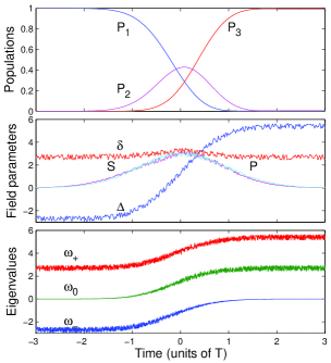
Figure 4: Same as Fig. 1 but for $\Omega_{0}=5.4/T$, $\alpha=0.1$, and $\beta=1.25$, and with fluctuations for the amplitudes and instantaneous frequencies. The field parameters and eigenvalues are shown for a single realization.

V Implementation of parallel STIRAP by pulse shaping techniques

The implementation of the parallel STIRAP requires the design of the pulses and frequencies using the state-of-the-art technology of pulse shaping, such as for instance liquid cristal spatial light modulators. Two such modulators allow the independent shaping of the spectral phase and amplitude of an input femtosecond laser pulse Weiner ; Chatel . We consider here for simplicity a constant two-photon detuning ($\alpha=0$). In that case, we have to chirp both field frequencies exactly in the same way. The difference between the two fields is their mean frequency and their delayed envelope. We can determine approximate curve fitting of the envelopes for $\alpha=0$:

$$\Omega_{P,S}(t)\approx\frac{\Omega_{0}}{2}\beta e^{-[(t\pm 0.14T)/(\beta T)]^{2}},\quad\beta=\sqrt{\frac{\pi}{2}}$$ (9)

with $+$ ($-$) holding respectively for the Stokes (pump) field. Figure 5 shows, for these fields of phase corresponding to (5) with $\alpha=0$ (cf. conditions of Fig. 1), their corresponding spectral amplitudes and phases, respectively denoted $A(\omega)$ and $\phi(\omega)$, and defined through the complex field as ${\cal E}\Lambda(t)e^{i\varphi(t)}=\frac{1}{2\pi}\int d\omega A(\omega)e^{i[\omega t+\phi(\omega)]}$ (for each field). Here $\varphi(t)$ is the instantaneous phase, leading the instantaneous frequency $d\varphi/dt$, $0\leq\Lambda(t)\leq 1$ the shape of the field amplitude, and ${\cal E}$ the peak amplitude of the considered field. The instantaneous frequencies of the pump field $\omega_{P}\equiv d\varphi_{P}/dt$ and of the Stokes field $\omega_{S}\equiv d\varphi_{S}/dt$ are connected to the one- and two-photon detunings as follows: $\omega_{P}(t)=\omega_{2}-\omega_{1}-\Delta(t)$, $\omega_{S}(t)=\omega_{2}-\omega_{3}+\delta-\Delta(t)$. We have chosen for convenience the mean frequency of the pump as $\omega_{0,P}=\omega_{2}-\omega_{1}-\Omega_{0}/4\equiv\omega_{P}(0)$ and of the Stokes as $\omega_{0,S}=\omega_{2}-\omega_{3}+\delta-\Omega_{0}/4\equiv\omega_{S}(0)$. We have considered fields of full width at half maximum $T_{\text{FWHM}}=500$ fs corresponding to $\Omega_{0}=17.1$ THz for the considered case $\Omega_{0}=5.8/T$. For typical transition strengths of 1 Debye, this leads to fields of peak intensities 15 GW/cm². For each field, the spectral parameters of Fig. 5 have been generated from a Gaussian Fourier transform limited pulse centered at the mean frequency $\omega_{0}$ with a full width at half maximum of 100 fs, shaped in phase and amplitude using two spatial light modulators. Note that we have considered the realistic effect of pixelization for the modulators (using 320 pixels, almost not noticeable at the scale of Fig. 5) which does not show any noticeable difference for the output pulses and the corresponding dynamics of Fig. 1.

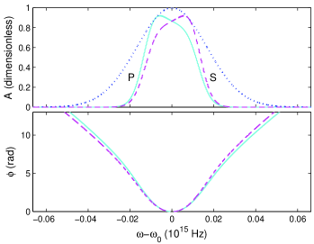
Figure 5: Tailored spectral normalized amplitudes $A$ (upper frame) and phases (lower frame) for the pump (full lines) and Stokes (dashed lines) fields from 100 fs Fourier transform limited pulses (upper frame, dotted line) of mean frequency $\omega_{0}$ to produce the fields of Fig. 1.

For practical implementation, it could be of interest to alternatively use, with the fitting Gaussian pulses (9), linearly chirped frequencies constructed from the linearization of (5) around $t=0$:

$$\Delta(t)=\frac{3\Omega_{0}}{2T\sqrt{\pi}}t,$$ (10)

where $\sqrt{\Omega_{P}^{2}+\Omega_{S}^{2}}$ is maximum. This would indeed allow one to use for instance gratings to produce the chirp instead of modulators (see for instance Noordam ). In this case, the duration of the pulse is connected to the slope of the chirp and the pulses have to be delayed additionally. Its efficiency is shown in Figs. 3 and 3: It is not as efficient as the level line strategy but is still well superior to the standard STIRAP. For instance, one can see that the deviation from the complete transfer is less than $10^{-2}$ with a pulse area larger than 3.5$\pi$ for this linearization, corresponding to a fluence larger than $10^{1.6}/T$. One recovers this accuracy for STIRAP for a fluence larger than 10.5$\pi$, corresponding to a fluence larger than $10^{2.5}/T$ (almost one order of magnitude larger). This linearization also allows an error smaller than 10^-4 for an area larger than 10$\pi$ (it should be larger than only 5.5$\pi$ for parallel STIRAP). Such accuracy is not reachable using the conventional STIRAP.

VI Conclusion and discussions

In conclusion, we have developed a strategy of adiabatic passage in $\Lambda$-systems with field designed such that the eigenvalues stay parallel at each time. This strategy allows one to combine the energetically efficiency of “$\pi$-pulse” and related strategies with the robustness of adiabatic passage. It has been shown in particular to be superior to the conventional STIRAP. It is expected to be easily implementable using modern tools of pulse shaping.

To implement the proposed strategy in real systems, one has to consider several limitations due to the presence of other states and to lossy processes such as ionization. In order to avoid the latter, the requirements are to consider a system which does not show a one-photon resonance into the continuum from the excited state and to use moderate field intensities, typically not more than 100 GW/cm² for atoms. Additional non-resonant states lead to Stark shifts which can be considered in general negligible with respect to the one-photon resonances considered here. However for the considered field intensities, they can play a role in deforming the dressed energies. In that case one has to recalculate the field parameters such that the eigenenergies stay parallel. The conditions that permit these additional states to stay non resonant can be estimated as $\Delta^{(j)}_{k}T\gg 1$ and $\Omega_{k}^{(j)}\lesssim\Delta^{(j)}_{k}$ with $\Delta^{(j)}_{k}$ the one-photon detuning for the state $j$ and the field $k$ and $\Omega_{k}^{(j)}$ the corresponding peak Rabi frequency.

This parallel adiabatic passage strategy should be adapted to produce in an optimal way superpositions of states such as in the case of fractional STIRAP fstirap . This should find applications in quantum information processing, for instance to implement fast quantum gates or quantum algorithm (such as the implementation of the parallel adiabatic passage for the quantum search QS ). The high efficiency of the parallel strategy shown in Fig. 2 is compatible with such applications imposing severe limitations on the admissible error, typically on a level below $10^{-4}$ (see, e.g., Vasilev and references therein).

- (1) B.W. Shore, The Theory of Coherent Atomic Excitation (Wiley, New York, 1990); ”Coherent manipulations of atoms using laser light”, Acta Physica Slovaka 58, 243 (2008).
- (2) M. Shapiro and P. Brumer, Principles of the Quantum Control of Molecular Processes (Wiley, New York, 2003).
- (3) M. A. Nielson and I. L. Chuang, Quantum Computation and Quantum Information (Cambridge University Press, Cambridge, England, 2000.
- (4) L. Allen and J. H. Eberly, Optical Resonance and Two-Level Atoms (Dover, New York, 1987).
- (5) M. Holthaus and B. Just, Phys. Rev. A 49, 1950 (1994).
- (6) J. Oreg, F. T. Hioe, and J. H. Eberly, Phys. Rev. A 29, 690 (1984); U. Gaubatz et al., J. Chem. Phys. 92, 5363 (1990).
- (7) N.V. Vitanov, T. Halfmann, B.W. Shore and K. Bergmann, Annu. Rev. Phys. Chem. 52, 763 (2001).
- (8) P. Král, I. Thanopulos, and M. Shapiro, Rev. Mod. Phys. 79, 53 (2007).
- (9) S. Guérin and H.R. Jauslin, Adv. Chem. Phys 125, 147 (2003).
- (10) S. Guérin, S. Thomas, and H.R. Jauslin, Phys. Rev. A 65, 023409 (2002).
- (11) U. Boscain, G. Charlot, J.-P. Gauthier, S. Guérin, and H. R. Jauslin, J. Math. Phys. 43, 2107 (2002).
- (12) S. Guérin, L. P. Yatsenko and H. R. Jauslin, Phys. Rev. A 63, 031403(R) (2001); L. P. Yatsenko, S. Guérin and H. R. Jauslin, Phys. Rev. A 65, 043407 (2002).
- (13) A. M. Weiner, Rev. Sci. Instrum. 71, 1929 (2000)
- (14) A. Monmayrant and B. Chatel, Rev. Sci. Instrum. 75, 2668 (2004).
- (15) T. Brixner and G. Gerber, Physica Scripta T110, 101 (2004).
- (16) N. Dudovich, T. Polack A. Pe’er, and Y. Silberberg, Phys. Rev. Lett. 94, 083002 (2005).
- (17) M. Aeschlimann, M. Bauer, D. Bayer, T. Brixner, F.J. Garc a de Abajo, W. Pfeiffer, M. Rohmer, C. Spindler, and F. Steeb, Nature 446, 301 (2007).
- (18) M. Wollenhaupt, A Präkelt, C. Sarpe-Tudoran, D. Liese and T. Baumert, J. Phys. B 41, 074007 (2008).
- (19) S. Guérin, A. Rouzée, and E. Hertz, Phys. Rev. A 77, 041404(R) (2008).
- (20) Y.B. Band and O. Magnes, Phys. Rev. A 50, 584 (1994).
- (21) I.R. Solá, V.S. Malinovsky, B.Y. Chang, J. Santamaria, and K. Bergmann, Phys. Rev. A 59, 4494 (1999).
- (22) M.P. Fewell, B.W. Shore, and K. Bergmann, Aust. J. Phys. 50, 281 (1997).
- (23) G. S. Vasilev, A. Kuhn, N. V. Vitanov, Phys. Rev. A 80, 013417 (2009).
- (24) D. J. Maas, C.W. Rella, P. Antoine, E.S. Toma, and L.D. Noordam, Phys. Rev. A 59, 1374 (1999).
- (25) N.V. Vitanov, K.-A. Suominen and B.W. Shore, J. Phys. B 32 4535 (1999).
- (26) D. Daems, S. Guérin, and N. Cerf, Phys. Rev. A 78, 042322 (2008).