Simulating Supersonic Turbulence in Magnetized Molecular Clouds

Abstract

We present results of large-scale three-dimensional simulations of weakly magnetized supersonic turbulence at grid resolutions up to $1024^{3}$ cells. Our numerical experiments are carried out with the Piecewise Parabolic Method on a Local Stencil and assume an isothermal equation of state. The turbulence is driven by a large-scale isotropic solenoidal force in a periodic computational domain and fully develops in a few flow crossing times. We then evolve the flow for a number of flow crossing times and analyze various statistical properties of the saturated turbulent state. We show that the energy transfer rate in the inertial range of scales is surprisingly close to a constant, indicating that Kolmogorov’s phenomenology for incompressible turbulence can be extended to magnetized supersonic flows. We also discuss numerical dissipation effects and convergence of different turbulence diagnostics as grid resolution refines from $256^{3}$ to $1024^{3}$ cells.

1 Introduction

Supersonic turbulence plays an important role in shaping hierarchical internal substructure of molecular clouds (MCs) [1, 2]. This turbulence is the key ingredient in statistical theories of star formation as it controls initial conditions for gravitationally collapsing objects [3, 4, 5]. The nature of molecular cloud turbulence is still poorly understood and no simple conceptual theory exists akin to that of Kolmogorov’s phenomenology for turbulence in fluids. Two major complications are strong compressibility of interstellar gas mediated by radiative energy losses and presence of dynamically important magnetic fields. While these two factors bring into play additional variables and equations rendering the modeling hardly tractable analytically and complicating numerical analysis, the nature of underlying nonlinearity contained in the advection terms remains the same. From a mathematician’s perspective, the general problem is essentially the same as in the Navier-Stokes turbulence, one of the remaining six unsolved Millennium Prize Problems for which the Clay Institute of Mathematics is offering a bonus of $1 million. Thus hopes to find universality in interstellar turbulence are not entirely unfounded, see e.g. [6], although some researchers believe that breakdown of universality in incompressible isotropic magnetohydrodynamic (MHD) turbulence is possible, e.g. due to nonlocality of interactions [7, 8].

The supersonic regime typical of MC turbulence is extremely hard to achieve in the laboratory and the information available from astronomical observations is rather limited [6]. This makes numerical simulations, perhaps, the only tool available to explore the statistics of supersonic turbulence in detail. High dynamic range simulations can shed light on the energy transfer between scales and on the key spatial correlations of the relevant fields in these flows only if they provide sufficient scale separation to resolve the dynamics of prevailing nonlinear interactions in the inertial range. In addition, low numerical dissipation and high-order numerical methods for three-dimensional compressible MHD are needed to achieve an accurate description of the inertial range of supersonic turbulence.

Stable, accurate, divergence-free simulation of magnetized supersonic turbulence is a severe test of numerical MHD schemes and has been surprisingly difficult to achieve due to the range of flow conditions present. Over the last two years we have developed Piecewise Parabolic Method on a Local Stencil (PPML), a new higher order-accurate, low dissipation numerical method which requires no additional dissipation or local “fixes” for stable execution [9, 10, 11]. PPML is a local stencil variant of the popular PPM algorithm [12] for solving the equations of compressible ideal magnetohydrodynamics. The principal difference between PPML and PPM is that cell interface states are “evolved” rather that reconstructed at every timestep, resulting in a compact stencil. Interface states are evolved using Riemann invariants containing all transverse derivative information. The scheme is fully multidimensional as the conservation laws are updated in an unsplit fashion, including the terms corresponding to the tangential directions in the amplitude equations. This helps to avoid numerous well-known pathologies, such as “carbuncles”, etc. [13]. Divergence-free evolution of the magnetic field is maintained using the higher order-accurate constrained transport technique [14]. The low dissipation and wide spectral bandwidth of this method make it an ideal choice for direct simulations of compressible turbulence.

In Ref. [15] we reported results from a set of three simulations of driven isothermal supersonic turbulence at a sonic Mach number of 10 on $512^{3}$ meshes demonstrating the performance of our PPML solver on models with different degrees of magnetization from super-Alfvénic through trans-Alfvénic regimes. Turbulence statistics derived from these three-dimensional models show that the density, velocity, and magnetic energy spectra vary strongly with the strength of turbulent magnetic field fluctuations. At the same time, the three cases suggest that a linear scaling in the 4/3-law of incompressible MHD turbulence [16, 17] is preserved even in the strongly compressible regime at $M_{s}=10$, if the proper density weighting is applied to the Elsässer fields following the 1/3-rule introduced in Refs. [15, 18, 23, 19], see Section 4.2 for more detail.

In this paper we present results from PPML simulations of statistically isotropic MHD turbulence at a sonic Mach number $M_{s}=10$ and Alfvénic Mach number $M_{A}=3$ on grids from $256^{3}$ to $1024^{3}$ cells. We use this set of simulations to check the (self-)convergence rates for various statistical measures with improved grid resolution. We also confirm the universal linear scaling for the mixed third-order structure functions of modified Elsässer fields discussed earlier in [15].

2 Numerical Model and Parameters

We use PPML to solve numerically the MHD equations for an ideal isothermal gas in a cubic domain of size $L=1$ with periodic boundary conditions

$$\frac{\partial\rho}{\partial t}+{\bf\nabla}\cdot(\rho{\bf u})=0,$$ (1)

$$\frac{\partial\rho{\bf u}}{\partial t}+{\bf\nabla\cdot}\left[\rho{\bf uu}-{\bf BB}+\left(p+\frac{{\bf B}^{2}}{2}\right){\bf I}\right]={\bf F},$$ (2)

$$\frac{\partial{\bf B}}{\partial t}+{\bf\nabla}\cdot({\bf uB}-{\bf Bu})=0.$$ (3)

Here $\rho$ and ${\bf u}$ are the gas density and velocity, ${\bf B}$ is the magnetic field, the gas pressure $p\equiv c_{s}^{2}\rho$ and the isothermal sound speed $c_{s}\equiv 1$, ${\bf I}$ is the unit tensor. PPML conserves mass, momentum and magnetic flux, and keeps ${\bf\nabla\cdot B}=0$ to the machine precision. A fixed large-scale ($k\leq 2$) isotropic nonhelical solenoidal force ${\bf F}\equiv\rho{\bf a}-\left<\rho{\bf a}\right>$, where ${\bf a}$ is the acceleration and $\left<\ldots\right>$ indicates averaging over the entire computational domain, is used to stir the gas keeping $M_{s}$ close to 10 during the simulation. The models are initiated with a uniform density $\rho_{0}\equiv 1$, large-scale velocity field ${\bf u}_{0}=\tau{\bf a}$, where $\tau$ is a constant such that $\left<{\bf u}_{0}^{2}\right>^{1/2}=8$, and a uniform magnetic field ${\bf B_{0}}$ aligned with the $x$-coordinate direction. The magnetic field strength is parameterized by the ratio of thermal-to-magnetic pressure $\beta_{0}\equiv p_{0}/{\bf B_{0}}^{2}$. In Ref. [15] we carried out three pilot simulations with $\beta_{0}=0.2$, 2, and 20 at $512^{3}$. Here we present results for three simulations with $\beta_{0}=2$ and grid resolutions $256^{3}$, $512^{3}$, and $1024^{3}$ cells. The largest of these three experiments was carried out using 2048 cores of Ranger supercomputer at TACC.

Our numerical experiments covered the transition to turbulence and evolution for up to eight dynamical times, $t_{d}\equiv L/2M_{s}$. The magnetic field was not forced and receives energy passively through interaction with the velocity field. This random forcing does not generate a mean field, but still leads to amplification of the small-scale magnetic energy through compression in shocks in combination with flux freezing and, possibly to some extent, via a process known as small-scale dynamo, e.g. [20] and references therein. It is implicitly assumed that the effective magnetic Prandtl number $P_{M}\approx 1$ in our numerical models. This is far from the realistic values for the interstellar conditions, where $P_{M}\gg 1$. The limitations imposed by the available computational resources allow us to reach effective Reynolds numbers on the order of $10^{4}$ in our largest MHD simulations, while the realistic values for molecular clouds can be as large as $\sim 10^{8}$.

3 The Saturated Turbulent State and Convergence

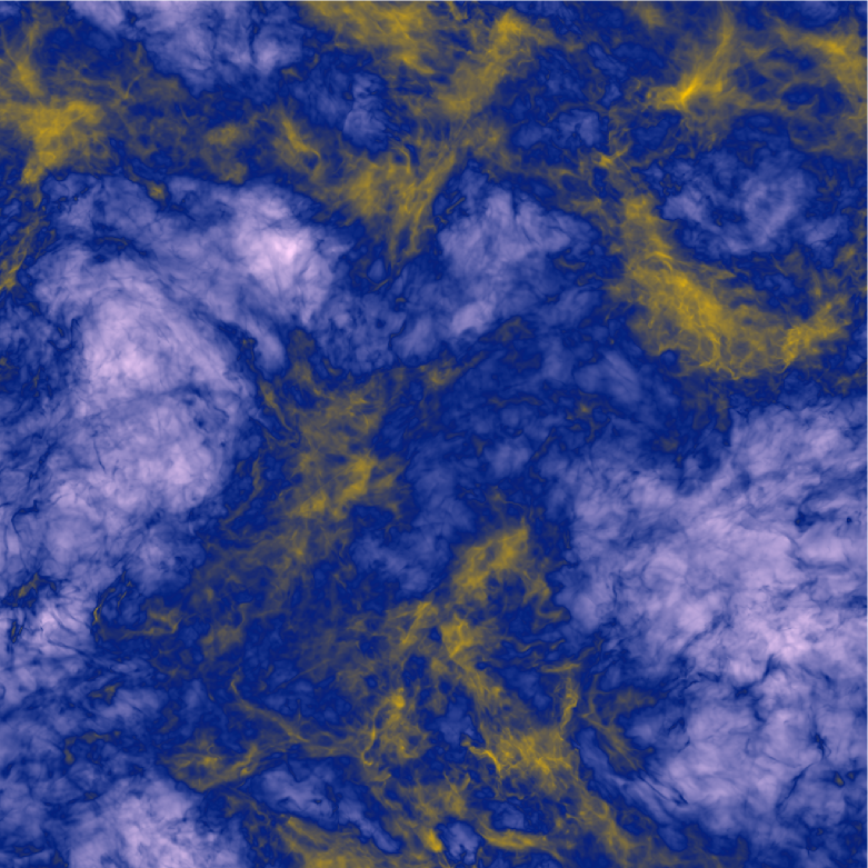
Figure 1: Projected (column) density image for a snapshot at $t=6.35t_{d}$ from a $1024^{3}$ PPML simulation of MHD turbulence at $M_{s}=10$ and $M_{A}=3$ carried out on Ranger (TACC) using 2048 cores. White-blue-yellow colors correspond to low-intermediate-high projected density values. The dynamic range of the image is about 100.

After the initial stir-up phase, our simulations reach a statistical steady state. A snapshot of the projected (column) density in such a saturated state is shown in Fig. 1. The morphology of structures visible in this projected density distribution is surprisingly similar to that from a non-magnetized simulation at $M_{s}=6$ presented in Fig. 1. of Ref. [15], even though the power spectrum index is about $-1.7$ here (see Section 4.1 and Fig. 3d) and $-2.0$ there (see Fig. 2a in Ref. [15]) and the morphology of the density distribution in thin slices (not shown) is clearly different. This illustrates the loss of information in the projection procedure that makes it difficult to measure physical parameters of supersonic turbulent flows from the observed projected density distributions alone.

The properties of this saturated state representing fully developed macroscopically isotropic compressible MHD turbulence are the main focus of this paper. While some level of physical understanding of small-scale rms field amplification and its saturation exists, the structure of the saturated state is poorly known, even in the incompressible case [7].

We compared the saturation levels for several integral characteristics of turbulence for models with three different resolutions: $256^{3}$, $512^{3}$, and $1024^{3}$. Since in the $\beta_{0}=2$ case the kinetic energy $E_{K}\equiv\int\frac{1}{2}\rho u^{2}dV$ dominates over the magnetic energy $E_{M}\equiv\int\frac{1}{2}B^{2}dV$ by a factor of about 3, it is practical to consider $E_{K}$ and $E_{M}$ separately instead of concentrating on the total energy $E_{T}=E_{K}+E_{M}$. Figure 2a shows that the kinetic energy is already converged on $256^{3}$ grids, in agreement with [21]. In contrast, the saturation level of magnetic energy at $\beta_{0}=2$ clearly depends on the grid resolution and there are good chances that convergence can be reached already at resolution of $2048^{3}$ cells. The mean values of $E_{M}$ for $t\in[3,7]$ are 10.0, 12.3, and 13.5 with the highest corresponding to our finest grid resolution of $1024^{3}$. The lack of convergence in $E_{M}$ stems from numerical diffusion suppressing small-scale compressions and also the small-scale dynamo action, if any, in low-resolution runs. The mean value of $E_{K}$ for the same averaging interval is 39.8, thus the magnetic energy contributes about one quarter of the total energy, $E_{M}/E_{T}\approx 0.25$, in the $1024^{3}$ model.

While the root mean square (rms) sonic Mach number $M_{s}$ saturates at a level of about 9.2 independent of the grid resolution, the Alfvén Mach number $M_{A}\approx 4.0$, 3.1, and 2.8 for grids with $256^{3}$, $512^{3}$, and $1024^{3}$ cells, respectively (see Fig. 2b). With the same initial uniform field ${\bf B}_{0}$, we get turbulent states with slightly different $M_{A}$ values with a tendency towards less super-Alfvénic flows at higher grid resolutions.

Figure 2: Statistics of MHD turbulence at $M_{s}=10$ and $\beta_{0}=2$, from PPML simulations at grid resolution of $256^{3}$, $512^{3}$, and $1024^{3}$ cells: (a) mean kinetic, magnetic, and residual energy ($\sigma_{R}\equiv(E_{K}-E_{M})/E_{T}$) vs. time; (b) rms sonic and Alfvénic Mach numbers; (c) mean and rms helicity; (d) mean and rms cross-helicity; (e) rms gas density; (f) compensated density power spectra at $t=3.5t_{d}$; (g) compensated velocity power spectra at $t=3.5t_{d}$; (h) compensated magnetic energy power spectra at $t=3.5t_{d}$.

Since we do not include the explicit dissipative terms in the equations we integrate numerically, the dissipation in our models is purely numerical and the higher resolution models correspond to higher effective Reynolds numbers. This can be traced in the non-converging levels of rms helicity gradually growing with higher grid resolution, see Fig. 2c. Since our driving force is non-helical to a very good approximation, the mean helicity stays close to zero over the course of a simulation. Figure 2d shows a rather slow convergence in the levels of the rms cross-helicity and finite deviations of the mean cross-helicity $H_{C}\equiv\int{\bf u\cdot B}dV$ from zero in low resolution runs. PPML does not exactly conserve cross-helicity, even though it is one of the ideal invariants in MHD. The normalized mean cross-helicity is, however, contained within $\pm 0.8$% for $\beta_{0}=2$ at $1024^{3}$. Even though both the kinetic and the magnetic energy as well as the rms Alfvén Mach number reach saturation after about 3 dynamical times of evolution in our models with $\beta_{0}=2$, the rms cross-helicity continues to grow slowly for up to 4 or even 5 dynamical times meaning that stirring the flow for $3t_{d}$ might not be sufficient to reach a statistical steady state.

Another global diagnostic to look at is the rms density. In models with higher resolution the flow is better resolved and higher level of density fluctuations is observed. The rms denstity is, however, not very sensitive to the grid resolution and changes from 2.2 to 2.3 as the resolution jumps from $256^{3}$ to $1024^{3}$, see Fig. 2e.

Finally, to illustrate the convergence of spectral properties of turbulent fluctuations, in Fig. 2f, g, and h we show compensated power spectra of the density, the velocity, and the magnetic field for a set of snapshots from simulations with different resolutions taken early in the saturated state at $t=3.5t_{d}$. The velocity spectra can be used to access the spectral bandwidth of PPML. As one can see from Fig. 2g, the velocity spectrum is resolved up to $\log_{10}k/k_{min}\approx 1.1$ at $256^{3}$ and up to $\log_{10}k/k_{min}\approx 1.4$ at $512^{3}$, consistent with the grid refinement by a factor of two.

4 Exploring Scaling Laws in Supersonic MHD Turbulence

Here we present time-averaged statistics for our highest resolution $\beta_{0}=2$ model at $1024^{3}$ grid cells and compare these with our previous results for non-magnetized (HD) simulations at $M_{s}=6$ and grid resolutions of $1024^{3}$ and $2048^{3}$ cells [18, 23, 15]. Our MHD data are based on 100 full data snapshots equally spaced in time for $t\in[3,8]t_{d}$, i.e. we do the averaging over five dynamical times which makes it, perhaps, the best available sample for compressible MHD turbulence at this resolution. Our projected density spectra are based on a sample of 750 projections, including all three projection directions, covering the same time span $t\in[3,8]t_{d}$. We first begin with the scaling properties of the basic fields, such as the density, velocity, and magnetic field and then discuss ideal invariants, such as the total energy and the energy transfer rate that may or may not display universal behavior.

4.1 Basic Fields

The probability density function (pdf) of the gas density is one of the most important inputs for the theories of star formation in molecular clouds as it determines the amount of the dense material available for gravitational collapse to form stars [3, 24, 5]. The ability to predict the pdf is important in other extreme astrophysical environments, such as, e.g., accretion onto “seed” black holes in the first galaxies [25]. It is also known as one of the most robust statistical characteristics for compressible isothermal turbulence as its lognormal shape [26, 27, 28, 29] gets quickly established in numerical simulations, e.g. [18]. Here we demonstrate the lognormal form of the pdf in our $\beta_{0}=2$ model which gives a perfect fit for a range of $\sim 10^{8}$ in probability at high densities (Fig. 3a). Compared to the unmagnetized cases at $M_{s}=6$ studied in [18, 15], the lognormal distribution in the MHD case with $M_{s}=10$ is, as expected at higher Mach numbers, somewhat wider. If we parametrize the standard deviation $\sigma$ as a function of the rms sonic Mach number, $\sigma^{2}\equiv\ln(1+b^{2}M_{s}^{2})$, we get $b=0.22$ and 0.27 as the best fit values for $\log_{10}\rho\in[-1,2.8]$ in the MHD and HD cases, respectively. The mean of the distrubution is also a function of the standard deviation, $\left<\ln\rho\right>=-\frac{1}{2}\sigma^{2}$. For more detail on the dependence of the pdf on the value of $\beta_{0}$ see [15].

The density power spectrum (Fig. 3b) scales roughly as $k^{-2/3}$, shallower than the slope of $-1$ in the HD case at a smaller $M_{s}=6$ [18]. The power spectrum of the logarithm of density (Fig. 3c) scales somewhat steeper, $k^{-4/3}$, but still shallower than $-5/3$ found at $M_{s}=6$ [15]. The power spectrum of the logarithm of projected gas density roughly follows the scaling $k^{-5/3}$, which is somewhat steeper than the scaling of the density power spectrum (Fig. 3d), but still shallower than $-2$ measured for the HD case at $M_{s}=6$ [15]. The sensitivity of the density spectra to the value of $\beta_{0}$ is discussed in detail in [15].

Figure 3: Time-average statistics of MHD turbulence at $M_{s}=10$ and $\beta_{0}=2$, from PPML simulation at grid resolution $1024^{3}$ cells: (a) the gas density pdf and lognormal fits for $\log_{10}{\rho}\in[-1,2.8]$; (b) compensated power spectrum of the gas density; (c) as b, but for the logarithm density; (d) as b, but for the projected density and for the logarithm of projected density; (e) as b, but for the velocity and its solenoidal and dilatational parts; (f) ratio of dilatational to total velocity power $\chi_{C}$ as a function of wavenumber $k$; (g) compensated power spectra of total, kinetic, and magnetic energy. (h) compensated third-order structure functions $S_{3}(\ell)$ for generalized Elsässer fields ${\bf Z}^{\pm}$ from $512^{3}$ and $1024^{3}$ simulations.

The velocity power spectrum as well as the results of the Helmholtz decomposition of the velocity ${\bf u}$ into the solenoidal (${\bf\nabla\cdot u}_{s}\equiv 0$) and dilatational (${\bf\nabla}\times{\bf u}_{c}\equiv 0$) parts, ${\bf u}={\bf u}_{s}+{\bf u}_{c}$, are shown in Fig. 3e. The velocity power index is very close to $-3/2$ at $k/k_{min}$ around 30, the value proposed for an isotropic incompressible case with turbulent energy equipartition [30, 31], and the spectrum is dominated by the solenoidal component which follows the same scaling. Note that in the HD simulation of Ref. [18] this range of wavenumbers is buried under the bottleneck bump which is known to be much weaker, if exists at all, in the MHD models. At lower wavenumbers (but still within the inertial range), the velocity spectrum tends to get steeper, as should be expected for a strongly supersonic regime. The spectrum for the dilatational component of velocity is generally slightly steeper, as was previously reported for non-magnetized turbulence [32, 18]. Figure 3f compares the fraction of dilatational component in the velocity power, $\chi_{c}(k)\equiv P({\bf u}_{c},k)/P({\bf u},k)$, from our PPML MHD model at $\beta_{0}=2$ with those in our previous PPM $M_{s}=6$ HD runs at resolutions of $1024^{3}$ and $2048^{3}$ cells [18, 23, 15]. In both HD runs $\chi_{c}(k)\approx 1/3$ in the inertial range, even though we used different driving forces and different parameterizations for PPM diffusion in these simulations. The fact that $\chi_{c}(k)$ tends to be close to $1/3$ in isotropic flows at high Mach numbers can be explained by purely geometric considerations. At the same time, in our MHD model $\chi_{c}(k)\approx 1/4$ or even somewhat lower. A lower mean level of saturation for $\chi_{c}(k)$ in magnetized flows at high Mach numbers can be explained by the additional magnetic pressure term in the momentum conservation equation. A similar value for $\chi_{c}(k)$ was obtained in Ref. [21] for a model with stronger field ($\beta_{0}=0.02$) at the same grid resolution, cf. [33]. The $k^{2}$-compensated power spectra of dilatational velocities in Fig. 14 of Ref. [21], however, demonstrate an unusual rise of power near the Nyquist frequency that we do not observe in our simulations with PPML. Neither do we see such rise in our HD models with PPM (Fig. 3e). The origin of this sharp rise in compressions at high wavenumbers in simulations with the Athena code [34] is unclear.

4.2 Ideal Invariants

Since the total energy $E_{T}$ is a conserved quantity, it is instructive to follow its distribution as a function of scale, $E_{T}(k)\equiv\frac{1}{2}\left[P(\rho^{1/2}{\bf u},k)+P({\bf B},k)\right]$, see Fig. 3g. It appears that to a good approximation the total energy follows a simple scaling law $E_{T}(k)\sim k^{4/3}$. It is hard to believe, though, that this scaling exponent is universal. We have shown that in non-magnetized turbulence the power index for $P(\rho^{1/2}{\bf u},k)$ does depend on the rms Mach number of the flow [18]. In MHD models, the scaling of $E_{T}(k)$ would also depend on the saturation level of the magnetic energy. Nevertheless, it is interesting to see how a combination of the magnetic and kinetic energy, each of which do not display a clear extended scaling range (Fig. 3g) add up to result in an extended flat stretch of the total energy spectrum. Is this coincidental? Or is this a result of self-organization in supersonic super-Alfvénic MHD turbulence?

A better candidate for universal scaling is the energy transfer rate. Indeed, our HD simulations have shown that $P(\rho^{1/3}{\bf u},k)$ follows the Kolmogorov $-5/3$ scaling at $M_{s}=6$ [18]. There is a set of exact scaling laws for homogeneous and isotropic incompressible MHD turbulence analogous to the 4/5-law of Kolmogorov for ordinary turbulence in neutral fluids [35, 16, 17]. The MHD laws can be expressed in terms of Elsässer fields, ${\bf z}^{\pm}\equiv{\bf u}\pm{\bf B}/\sqrt{4\pi\rho}$ [36], as $S_{\parallel,3}^{\pm}\equiv\left<\delta z^{\mp}_{\parallel}(\ell)[\delta z_{i}^{\pm}(\ell)]^{2}\right>=-\frac{4}{d}\epsilon^{\pm}\ell$, where $\delta{\bf z}_{\parallel}(\ell)\equiv[{\bf z}({\bf x+\hat{e}}\ell)-{\bf z}({\bf x})]\cdot{\bf\hat{e}}$, $d$ is the space dimension, ${\bf\hat{e}}$ is a unit vector with arbitrary direction, ${\bf\hat{e}}\ell$ is the displacement vector, the brackets denote an ensemble average, and summation over repeated indices is implied. Equivalently, the scaling laws can be rewritten in terms of the basic fields (${\bf u}$, ${\bf B}$), but in MHD there are no separate exact laws for the velocity or the magnetic field alone. It is important not to neglect the correlations between the ${\bf u}$ and ${\bf B}$ fields or ${\bf z}^{+}$ and ${\bf z}^{-}$ fields constrained by the invariance properties of the equations in turbulent cascade models. In supersonic turbulence, it is equally important to properly account for the density–velocity and density–magnetic field correlations. In incompressible MHD, the total energy $E_{T}$ and the cross-helicity $H_{C}$ play the role of ideal invariants and, thus, the (total) energy transfer rate $\epsilon^{T}=(\epsilon^{+}+\epsilon^{-})/2$ and the cross-helicity transfer rate $\epsilon^{C}=(\epsilon^{+}-\epsilon^{-})/2$. For vanishing magnetic field ${\bf B}$, one recovers the Kolmogorov 4/5-law, $\left<[\delta{\bf u}_{\parallel}(\ell)]^{3}\right>=-4/5\epsilon\ell$, where $\epsilon$ is the mean rate of kinetic energy transfer [17].

Numerical simulations generally confirm these incompressible scalings, although the Reynolds numbers are perhaps still too small to reproduce the asymptotic linear behavior with a desired precision and the results are sensitive to statistical errors [37, 32, 38]. Often, the absolute value of the longitudinal difference is used and still a linear scaling is recovered numerically, while there is no rigorous result for the normalization constant in this case. The third-order transverse velocity structure functions also show a linear scaling in simulations of nonmagnetized turbulence [32, 18] and the difference of scaling exponents for longitudinal and transverse structure functions can serve as a robust measure of statistical uncertainty of the computed exponents [39]. In MHD simulations, the third-order structure functions of the Elsässer fields $\left<|\delta z^{\mp}_{\parallel}(\ell)|^{3}\right>$ were shown to have an approximately linear scaling too [37, 40], but again there is no reason for this result to universally hold in all situations since the correlations between the ${\bf z}^{\pm}$ fields play an important role in nonlinear transfer processes.

Can the 4/3-law for incompressible MHD turbulence be extended to supersonic regimes in molecular clouds? As we discussed in Ref. [15], a proper density weighting of the velocity, $\rho^{1/3}{\bf u}$, preserves the approximately linear scaling of the third-order structure functions at high Mach numbers in the nonmagnetized case (for a more involved approach to density weighting see Ref. [41]). It is straightforward to redefine the Elsässer fields for compressible flows using this “1/3-rule”, ${\bf Z}^{\pm}\equiv\rho^{1/3}({\bf u}\pm{\bf B}/\sqrt{4\pi\rho})$, so that they match the original ${\bf z}^{\pm}$ fields in the incompressible limit and reduce to $\rho^{1/3}{\bf u}$ in the limit of vanishing ${\bf B}$. The new ${\bf Z}^{\pm}$ fields can have universal scaling properties in homogeneous isotropic turbulent flows with a broad range of sonic and Alfvénic Mach numbers.

We use data from our $1024^{3}$ MHD simulation to support the conjecture proposed in Ref. [15] and compute the third-order structure functions $S_{\parallel,3}^{\pm}$ and $S_{\perp,3}^{\pm}$ defined above using the ${\bf Z}^{\pm}$ fields. Since we are interested in the energy transfer through the inertial interval, we compute the sum of $S_{\parallel,3}^{-}$ and $S_{\parallel,3}^{+}$ which determines the energy transfer rate $\epsilon^{T}$ in the incompressible limit. To further reduce statistical errors, we combine the transverse and longitudinal structure functions, but the absolute value operator was not applied to the field differences. Figure 3h shows the compensated scaling for $S_{3}(\ell)\equiv(S_{\parallel,3}^{-}+S_{\parallel,3}^{+}+S_{\perp,3}^{-}+S_{\perp,3}^{+})/4$ averaged over 100 flow snapshots and the best linear fit $S_{3}(\ell)\sim\ell^{1.020\pm 0.001}$ for $\log{\ell/\Delta}\in[1.1,1.8]$. For comparison, we overplot data from our $512^{3}$ simulation discussed in Ref. [15]. Clearly, at $1024^{3}$, we get a more extended scaling range and confirm the linear scaling found in [15]. Howefer, further work is needed to verify this result with high resolution simulations at different levels of magnetization.

5 Conclusions

We verified the applicability of the 1/3-rule of hydrodynamic supersonic turbulence to super-Alfvénic regimes of MHD turbulence using data from a new simulation with the Piecewise Parabolic Method on a Local Stencil on a grid of $1024^{3}$ cells. Our results suggest that the energy transfer rate is approximately constant accross the inertial interval and that the 4/3-law of incompressible MHD can be extended to the supersonic turbulent flows.

This research was supported in part by the National Science Foundation through grants AST-0607675 and AST-0808184, as well as through TeraGrid resources provided by NICS, PSC, SDSC, and TACC (MCA07S014 and MCA98N020).

References

References

- [1] Elmegreen B G and Scalo J 2004 ARA&A 42 211–73 (Preprint arXiv:astro-ph/0404451)
- [2] Scalo J and Elmegreen B G 2004 ARA&A 42 275–316 (Preprint arXiv:astro-ph/0404452)
- [3] Padoan P and Nordlund Å 2002 ApJ 576 870–79 (Preprint arXiv:astro-ph/0011465)
- [4] McKee C F and Ostriker E C 2007 ARA&A 45 565–687
- [5] Padoan P, Nordlund Å, Kritsuk A G, Norman M L and Li P S 2007 ApJ 661 972–81 (Preprint arXiv:astro-ph/0701795)
- [6] Heyer M H and Brunt C M 2004 ApJL 615 L45–8 (Preprint arXiv:astro-ph/0409420)
- [7] Yousef T A, Rincon F and Schekochihin A A 2007 Journal of Fluid Mechanics 575 111
- [8] Beresnyak A and Lazarian A 2009 ArXiv e-prints (Preprint arXiv:0904.2574)
- [9] Popov M V and Ustyugov S D 2007 Computational Mathematics and Mathematical Physics 47 1970–89
- [10] Popov M V and Ustyugov S D 2008 Computational Mathematics and Mathematical Physics 48 477–99
- [11] Ustyugov S D, Popov M V, Kritsuk A G and Norman M L 2009 Preprint arXiv:0905.2960
- [12] Colella P and Woodward P R 1984 J. Comp. Phys. 54 174–201
- [13] Quirk J J 1994 International Journal for Numerical Methods in Fluids 18 555–74
- [14] Gardiner T A and Stone J M 2005 J. Comp. Phys. 205 509–39 (Preprint arXiv:astro-ph/0501557)
- [15] Kritsuk A G, Ustyugov S D, Norman M L and Padoan P 2009 ASP Conference Series 406 15–22
- [16] Politano H and Pouquet A 1998 Phys. Rev. E 57 21
- [17] Politano H and Pouquet A 1998 Geophysical Research Letters 25 273–6
- [18] Kritsuk A G, Norman M L, Padoan P and Wagner R 2007 ApJ 665 416–31 (Preprint arXiv:0704.3851)
- [19] Kowal G and Lazarian A 2007 ApJL 666 L69–72 (Preprint arXiv:0705.2464)
- [20] Schekochihin A A and Cowley S C 2007 Turbulence and Magnetic Fields in Astrophysical Plasmas (Magnetohydrodynamics: Historical Evolution and Trends) p 85
- [21] Lemaster M N and Stone J M 2009 ApJ 691 1092–108 (Preprint arXiv:0809.4005)
- [22] Sytine I V, Porter D H, Woodward P R, Hodson S W and Winkler K H 2000 J. Comp. Phys. 158 225–38
- [23] Kritsuk A G, Padoan P, Wagner R and Norman M L 2007 AIP Conf. Proc. 932 393–9
- [24] Krumholz M R and McKee C F 2005 ApJ 630 250–268 (Preprint arXiv:astro-ph/0505177)
- [25] Milosavljević M, Bromm V, Couch S M and Oh S P 2009 ApJ 698 766–780 (Preprint arXiv:0809.2404)
- [26] Vazquez-Semadeni E 1994 ApJ 423 681
- [27] Padoan P, Nordlund A and Jones B J T 1997 MNRAS 288 145–52
- [28] Nordlund Å K and Padoan P 1999 The Density PDFs of Supersonic Random Flows Interstellar Turbulence ed Franco J and Carraminana A p 218
- [29] Biskamp D 2003 Magnetohydrodynamic Turbulence (Cambridge University Press)
- [30] Iroshnikov P S 1963 Astronomicheskii Zhurnal 40 742
- [31] Kraichnan R H 1965 Physics of Fluids 8 1385–87
- [32] Porter D H, Pouquet A and Woodward P R 2002 Phys. Rev. E 66 026301
- [33] Boldyrev S, Nordlund Å and Padoan P 2002 Phys. Rev. Lett. 89 031102 (Preprint arXiv:astro-ph/0203452)
- [34] Stone J M, Gardiner T A, Teuben P, Hawley J F and Simon J B 2008 ApJS 178 137–77 (Preprint arXiv:0804.0402)
- [35] Chandrasekhar S 1951 Proc. Royal Society London, Ser. A 204 435–49
- [36] Elsässer W M 1950 Physical Review 79 183
- [37] Biskamp D and Müller W C 2000 Physics of Plasmas 7 4889–900
- [38] Boldyrev S, Mason J and Cattaneo F 2006 Preprint arXiv:astro-ph/0605233
- [39] Kritsuk A G and Norman M L 2004 ApJL 601 L55–8 (Preprint arXiv:astro-ph/0310697)
- [40] Momeni M and Mahdizadeh N 2008 Physica Scripta Volume T 131 014004
- [41] Pan L, Padoan P and Kritsuk A G 2009 Phys. Rev. Lett. 102 034501–4 (Preprint arXiv:0808.1330)