The Quantum Normal Form Approach to Reactive Scattering: The Cumulative Reaction Probability for Collinear Exchange Reactions

Abstract

The quantum normal form approach to quantum transition state theory is used to compute the cumulative reaction probability for collinear exchange reactions. It is shown that for heavy atom systems like the nitrogen exchange reaction the quantum normal form approach gives excellent results and has major computational benefits over full reactive scattering approaches. For light atom systems like the hydrogen exchange reaction however the quantum normal approach is shown to give only poor results. This failure is attributed to the importance of tunnelling trajectories in light atom reactions that are not captured by the quantum normal form as indicated by the only very slow convergence of the quantum normal form for such systems.

I Introduction

The classical mechanical picture of a chemical reaction as a scattering problem across a saddle point of the Born-Oppenheimer potential energy surface in configuration space has proven to be a fruitful way of visualizing and thinking about chemical reactions since the 1930’s, when Eyring, Polanyi, and Wigner developed transition state theory (TST). TST provides the framework for computing, using classical mechanics, many of the physically important quantities for describing such chemical reactions. The fundamental geometrical object in TST is a dividing surface that divides the energy surface into a reactant and a product component. With such a dividing surface in hand, one can then compute the reaction rate from the directional phase space flux through this surface. In order not to overestimate the rate the dividing surface must not be recrossed by reactive trajectories, i.e. the dividing surface should have the “no re-crossing” property. In the 70’s Pechukas, Pollak and others PechukasMcLafferty73 ; PechukasPollak78 showed that for two degrees of freedom such a dividing surface can be constructed from a periodic orbit (the so called periodic orbit dividing surface). Recently it has been shown that for more than two degrees-of-freedom a dividing surface that is free of recrossings can be built from a normally hyperbolic invariant manifold (NHIM) Wiggins94 . The dividing surface and the NHIM can be directly constructed from an algorithm based on a Poincaré-Birkhoff normal form procedure UJPYW01 which also gives an expression for the flux WaalkensWiggins04 . The classical phase space transition state theory, based on Poincaré-Birkhoff normal form theory, naturally leads to a quantum version of transition state theory, based on a quantum normal form. Since the normal form is valid in a neighborhood in energy both above and below the saddle point, it includes the quantum effect of tunneling in the region near the saddle. Moreover, it does not require a full quantum simulation in a neighborhood of the TST dividing surface (schubert_prl ; wsw08 ) in order to compute important quantities associated with the reaction. This is significant since much effort has been devoted to developing a quantum version of transition state theory whose implementation remains feasible for multi-dimensional systems (see the flux-flux autocorrelation function formalism by Miller and coworkers Miller98 ). However, in Miller1 Miller stated that “–the conclusion of it all is that there is no uniquely well defined quantum version of TST in the sense that there is in classical mechanics. This is because tunneling along the reaction coordinate necessarily requires one to solve the (quantum) dynamics for some finite region about the TS dividing surface, and if one does this quantum mechanically there is no ‘theory’ left, i.e., one has a full dimensional quantum dynamics treatment that is ipso facto exact, a quantum simulation.” Nevertheless, our approach based on the quantum normal form leads to a quantum version of transition state theory that includes tunneling near the saddle and does not require a full quantum simulation in a neighborhood of the TST dividing surface. Moreover, our computation of the cumulative reaction probability can be viewed as the quantum mechanical flux through a (classically recrossing free) dividing surface, which includes tunneling. The quantum normal form gives a local decoupling of the quantum dynamics to any desired order in $\hbar$ which is the key issue here, i.e. locally, we have a decoupling of the scattering states into forward/backward reactive and non-reactive, and for these states we know the transmission probabilities analytically. Therefore we do not have to ‘simulate’ the quantum dynamics. Hence, it sidesteps the issues and concerns expressed by Miller.

In this paper we illustrate the utility of the quantum normal form approach to quantum transition state theory by considering the computation and behavior of the bimolecular cumulative reaction probability (CRP) ${\mathcal{N}}(E)$, defined as seideman ; miller98

$${\mathcal{N}}(E)=\sum_{{\mathrm{\bf n}}_{\mathrm{r}},{\mathrm{\bf n}}_{\mathrm{p}}}|S_{{\mathrm{\bf n}}_{\mathrm{r}},{\mathrm{\bf n}}_{\mathrm{p}}}(E)|^{2},$$ (1)

where $S(E)$ is the reactive scattering matrix evaluated at energy $E$, and ${\mathrm{\bf n}}_{\mathrm{r}}$ (${\mathrm{\bf n}}_{\mathrm{p}}$) are the quantum numbers describing the asymptotic channel of incoming reactants (outgoing products). The CRP is a fundamental quantity that characterizes the reaction rate: the microcanonical and canonical rate constants can be determined from ${\mathcal{N}}(E)$ by means of simple relations seideman .

This paper is outlined as follows. In Section II we outline the theoretical and computational aspects of the quantum normal form theory. We emphasize the structural features that allow for the treatment of high dimensional quantum problems and show how the quantum normal form leads to a “simple” expression for the CRP. In Section III we apply the quantum normal form approach to the computation of the CRP for the collinear hydrogen and nitrogen exchange reactions. These quantities are compared to the “exact” answer obtained from a reactive quantum scattering calculation. In Section IV we discuss some aspects related to the convergence properties of the quantum normal form, and in Section V we summarize our results and offer some directions for further investigations.

II Quantum normal form theory

In this section we present central aspects of the quantum normal form (QNF) theory; for rigorous mathematical statements, proofs and further details we refer to Ref. schubert_prl ; wsw08 .

We begin by considering a quantum Hamilton operator $\hat{H}$ which we assume to be obtained from the Weyl quantization of a classical Hamilton function $H({\bf p},{\bf q})$. Here ${\bf q}=(q_{1},q_{2},\ldots,q_{d})$ and ${\bf p}=(p_{1},p_{2},\ldots,p_{d})$ denote the canonical coordinates and momenta, respectively, of a Hamiltonian system with $d$ degrees of freedom. Throughout this paper we will use atomic units, so that ${\bf q}$ and ${\bf p}$ are dimensionless. We will denote the corresponding operators by $\hat{{\bf q}}=(\hat{q}_{1},\hat{q}_{2},\ldots,\hat{q}_{d})$ and $\hat{{\bf p}}=(\hat{p}_{1},\hat{p}_{2},\ldots,\hat{p}_{d})$. In the coordinate representation their components correspond to multiplication by $q_{j}$ and the differential operators $\hat{p}_{j}=-\mathrm{i}\hbar_{\mathrm{eff}}\,\partial/\partial q_{j}$. Here $\hbar_{\mathrm{eff}}$ is a dimensionless parameter which corresponds to a scaled, effective Planck’s constant. For molecular reactions described in the Born-Oppenheimer approximation, $\hbar_{\mathrm{eff}}^{2}$ occurs naturally as the ratio of the electronic mass and the reduced mass of the nuclei participating in the reaction as we will see below in more detail.

The main idea of the QNF procedure is to approximate the Hamilton operator $\hat{H}$ by a simpler Hamilton operator obtained from a power series expansion of $\hat{H}$ which is simplified order by order using unitary transformations. As we will describe in more detail in Sec. IV the scaled Planck’s constant, $\hbar_{\mathrm{eff}}$, will play the role of a ‘small parameter’ which controls the quality of the QNF approximation. For our application of bimolecular reactions, the resulting transformed Hamilton operator truncated at a suitable order will be simpler in the sense that it will provide an easy, explicit way to compute the cumulative reaction probability.

To define and implement the unitary transformations it is extremely beneficial not to work with operators but with their Weyl symbols instead. The Weyl symbol of an operator $\hat{H}$ is defined as

$$H^{(0)}({\bf q},{\bf p};\hbar_{\mathrm{eff}})=\int\!d{\bf x}\,\langle{\bf q}-{\bf x}/2|\hat{H}|{\bf q}+{\bf x}/2\rangle\,e^{i{\bf p}{\bf x}/\hbar_{\mathrm{eff}}}.$$ (2)

The superscript $(0)$ is introduced for reasons that will become clear in a moment. The map $\hat{H}\mapsto H^{(0)}({\bf q},{\bf p};\hbar_{\mathrm{eff}})$ leading to (2) is also called the Wigner map. It is the inverse of the transformation which yields a Hamilton operator $\hat{H}$ from the Weyl quantization, $\mathrm{Op}[H]$, of a phase space function $H$ (the Weyl map) which, using Dirac notation, is given by

$$\begin{split}\hat{H}=\mathrm{Op}[H]=&\iint\frac{d{\bf q}d{\bf p}}{\left(2\pi\hbar_{\mathrm{eff}}\right)^{d}}H({\bf q},{\bf p})\\ &\times\displaystyle\int d{\bf x}|{\bf q}-{\bf x}/2\rangle e^{-i{\bf p}{\bf x}/\hbar_{\mathrm{eff}}}\langle{\bf q}+{\bf x}/2|\,.\end{split}$$ (3)

Accordingly, $H^{(0)}({\bf q},{\bf p};\hbar_{\mathrm{eff}})$ in (2) agrees with the classical Hamilton function $H({\bf q},{\bf p})$ in our case. The argument $\hbar_{\mathrm{eff}}$ is introduced for convenience since the Weyl symbol of the unitarily transformed Hamilton operator will in general explicitly depend on $\hbar_{\mathrm{eff}}$.

We will now assume that $H^{(0)}({\bf q},{\bf p};\hbar_{\mathrm{eff}})$ (or equivalently $H({\bf q},{\bf p})$) has a (single) equilibrium point, ${\bf z}_{0}\equiv({\bf q}_{0},{\bf p}_{0})$, of saddle-center-$\ldots$-center stability type. By this we mean that the matrix associated with the linearization of Hamilton’s equations about this equilibrium point has two real eigenvalues, $\pm\lambda$, of equal magnitude and opposite sign, and $d-1$ purely imaginary complex conjugate pairs of eigenvalues $\pm\mathrm{i}\omega_{k}$, $k=2,\ldots,d$. If the classical Hamiltonian is of the form kinetic energy plus potential energy then these type of equilibrium points of Hamilton’s equations correspond to index one saddle points of the potential energy. Using the symbol calculus the QNF theory provides a systematic procedure to obtain a local approximation, $\hat{H}_{\mathrm{QNF}}$, of the Hamiltonian $\hat{H}$ in a phase-space neighborhood of the equilibrium point ${\bf z}_{0}$ in order to facilitate further computation of various quantities, such as the CRP, of the reaction system under consideration. In the following we summarize the essential steps of the QNF procedure.

The QNF procedure consists of a sequence of, in general $\hbar_{\mathrm{eff}}$ dependent, generalized phase-space coordinate transformations changing the symbol as

$$H^{(0)}\rightarrow H^{(1)}\rightarrow H^{(2)}\rightarrow H^{(3)}\rightarrow\ldots\rightarrow H^{(N)}.$$ (4)

The first of the transformations (4) shifts the equilibrium point ${\bf z}_{0}$ to the origin according to

$$H^{(1)}({\bf z};\hbar_{\mathrm{eff}})=H^{(0)}({\bf z}+{\bf z}_{0};\hbar_{\mathrm{eff}})\,,$$ (5)

where ${\bf z}\equiv({\bf q},{\bf p})$. Once the equilibrium point is shifted to the origin, the QNF procedure deals with the Taylor expansion of the symbols in ${\bf z}$ and $\hbar_{\mathrm{eff}}$:

$$H^{(n)}({\bf z};\hbar_{\mathrm{eff}})=E_{0}+\sum_{s=2}^{\infty}H_{s}^{(n)}({\bf z};\hbar_{\mathrm{eff}})\,,$$ (6)

with

$$\begin{split}H_{s}^{(n)}({\bf z};\hbar_{\mathrm{eff}})=&\displaystyle\sum_{|\alpha|+|\beta|+2j=s}\frac{H_{\alpha_{1},\ldots,\alpha_{d},\beta_{1},\ldots,\beta_{d},j}^{(n)}}{\alpha_{1}!\ldots\alpha_{d}!\beta_{1}!\ldots\beta_{d}!j!}\\ &\times q_{1}^{\alpha_{1}}\ldots q_{d}^{\alpha_{d}}p_{1}^{\beta_{1}}\ldots p_{d}^{\beta_{d}}\,\hbar_{\mathrm{eff}}^{j}\,,\end{split}$$ (7)

where $\alpha_{k},\beta_{k},j\in\mathbb{N}_{0}$, $|\alpha|=\sum_{k}\alpha_{k}$, $|\beta|=\sum_{k}\beta_{k}$, and

$$H_{\alpha_{1},\ldots,\alpha_{d},\beta_{1},\ldots,\beta_{d},j}^{(n)}$$ (8)

$$=\displaystyle\left.\prod_{k,l=1}^{d}\frac{\partial^{\alpha_{k}}}{\partial q_{k}^{\alpha_{k}}}\frac{\partial^{\beta_{l}}}{\partial p_{l}^{\beta_{l}}}\frac{\partial^{j}}{\partial\varepsilon^{j}}H^{(n)}({\bf z};\varepsilon)\right|_{({\bf 0};0)}\!\!\!.$$

At the next step of the transformation sequence one finds a symplectic $2d\times 2d$ matrix $M$ such that the second order term of the symbol

$$H^{(2)}({\bf z};\hbar_{\mathrm{eff}})=H^{(1)}(M^{-1}{\bf z};\hbar_{\mathrm{eff}})$$ (9)

takes the particularly simple form:

$$H_{2}^{(2)}({\bf z};\hbar_{\mathrm{eff}})=\lambda q_{1}p_{1}+\sum_{k=2}^{d}\frac{\omega_{k}}{2}(q_{k}^{2}+p_{k}^{2})\,.$$ (10)

Section 2.3 of Ref. wsw08 provides an explicit procedure for constructing the transformation matrix $M$.

In order to proceed with the higher order transformations of the symbol of the Hamiltonian it is essential to introduce the notion of the Moyal bracket. Given two symbols $A({\bf z};\hbar_{\mathrm{eff}})$ and $B({\bf z};\hbar_{\mathrm{eff}})$, corresponding to operators $\hat{A}$ and $\hat{B}$ respectively, the Moyal bracket

$$\begin{split}\{A,B\}_{\mathrm{M}}=\frac{2}{\hbar_{\mathrm{eff}}}A\sin\left[\frac{\hbar_{\mathrm{eff}}}{2}\sum_{j=1}^{d}\left(\frac{\overleftarrow{\partial}}{\partial q_{j}}\frac{\overrightarrow{\partial}}{\partial p_{j}}-\frac{\overleftarrow{\partial}}{\partial p_{j}}\frac{\overrightarrow{\partial}}{\partial q_{j}}\right)\right]B\end{split}$$ (11)

gives the Weyl symbol of the operator $i[\hat{A},\hat{B}]/\hbar_{\mathrm{eff}}$, where $[\cdot,\cdot]$ denotes the commutator. The arrows in (11) indicate whether the partial differentiation acts to the left (on $A$) or to the right (on $B$). Equation (11) implies that, in general, for $\hbar_{\mathrm{eff}}\rightarrow 0$,

$$\{A,B\}_{\mathrm{M}}=\{A,B\}+\mathcal{O}(\hbar_{\mathrm{eff}}^{2})\,,$$ (12)

where $\{\cdot,\cdot\}$ denotes the Poisson bracket. Moreover, if at least one of the functions $A$, $B$ is a second order polynomial in the variables ${\bf q}$, ${\bf p}$ then $\{A,B\}_{\mathrm{M}}=\{A,B\}$. Finally, to simplify further notations we define the Moyal-adjoint operator as

$$\mathrm{Mad}_{A}:B\mapsto\mathrm{Mad}_{A}B\equiv\{A,B\}_{\mathrm{M}}\,.$$ (13)

Continuing with the sequence of transformations of the symbol in (4) we define the spaces

$$\mathcal{W}^{n}=\mathrm{span}\left\{q_{1}^{\alpha_{1}}\ldots q_{d}^{\alpha_{d}}p_{1}^{\beta_{1}}\ldots p_{d}^{\beta_{d}}\hbar_{\mathrm{eff}}^{j}:\right.$$ (14)

$$\left.\phantom{p_{d}^{\beta_{d}}+++++++}|\alpha|+|\beta|+2j=n\right\}\,.$$

Then, the symbol $H^{(n)}$ with $n\geq 3$ is obtained from $H^{(n-1)}$ by means of the transformation generated by a function $W_{n}({\bf z};\hbar_{\mathrm{eff}})\in\mathcal{W}^{n}$,

$$H^{(n)}=\sum_{k=0}^{\infty}\frac{1}{k!}\left[\mathrm{Mad}_{W_{n}}\right]^{k}H^{(n-1)}\,.$$ (15)

The structure of the transformation defined by Eq. (15) implies wsw08 that the operators $\hat{H}^{(n)}$ and $\hat{H}^{(n-1)}$ corresponding respectively (through the Weyl quantization) to the symbols $H^{(n)}$ and $H^{(n-1)}$ are related to one another by means of the unitary transformation $\hat{H}^{(n)}=e^{\mathrm{i}\hat{W}_{n}/\hbar_{\mathrm{eff}}}\hat{H}^{(n-1)}e^{-\mathrm{i}\hat{W}_{n}/\hbar_{\mathrm{eff}}}$, where $\hat{W}_{n}$ is the operator corresponding to the symbol $W_{n}$. In terms of the Taylor expansion defined in Eqs. (6-8) the transformation introduced by Eq. (15) reads

$$H^{(n)}_{s}=\sum_{k=0}^{\left\lfloor\frac{s}{n-2}\right\rfloor}\frac{1}{k!}\left[\mathrm{Mad}_{W_{n}}\right]^{k}H^{(n-1)}_{s-k(n-2)}\,,$$ (16)

where $\lfloor\cdot\rfloor$ gives the integer part of a number, i.e., the ‘floor’-function. Using Eq. (16) one can show that the transformation defined by Eq. (15) satisfies the following properties for $n\geq 3$:

$$H_{s}^{(n)}=H_{s}^{(n-1)}\,,\;\;\;\mathrm{for}\;\;\;s<n\,,$$ (17)

so that, in particular, $H_{2}^{(n)}=H_{2}^{(2)}$, and

$$H_{n}^{(n)}=H_{n}^{(n-1)}-\mathcal{D}W_{n}\,,$$ (18)

where

$$\mathcal{D}\equiv\mathrm{Mad}_{H_{2}^{(2)}}=\{H_{2}^{(2)},\cdot\}\>.$$ (19)

Equation (18) is referred as to the quantum homological equation.

We now specify the generating function $W_{n}$ by requiring $\mathcal{D}H_{n}^{(n)}=0$, or equivalently $H_{n}^{(n)}$ to be in the kernel of the restriction of $\mathcal{D}$ to $\mathcal{W}^{n}$; in view of Eq. (18) this condition yields

$$H_{n}^{(n-1)}-\mathcal{D}W_{n}\in\mathrm{Ker}\,\mathcal{D}|_{\mathcal{W}^{n}}\,.$$ (20)

Section 3.4.1 of Ref. wsw08 provides the explicit procedure of finding the solution of Eq. (20). Provided the linear frequencies $\omega_{2},\ldots,\omega_{d}$ in (10) are rationally independent, i.e. $m_{2}\omega_{2}+\ldots+m_{d}\omega_{d}=0$ implies $m_{2}=\ldots=m_{d}=0$ for all integers $m_{2},\ldots,m_{d}$, it follows that for odd $n$, $H_{n}^{(n)}=0$, and for even $n$,

$$H_{n}^{(n)}\in\mathrm{span}\left\{I^{\alpha_{1}}J_{2}^{\alpha_{2}}J_{3}^{\alpha_{3}}\ldots J_{d}^{\alpha_{d}}\hbar_{\mathrm{eff}}^{j}:|\alpha|+j=n/2\right\}\,,$$ (21)

where $I=q_{1}p_{1}$ and $J_{k}=(q_{k}^{2}+p_{k}^{2})/2$, with $k=2,\ldots,d$, are the analogues of the classical integrals.

Applying the transformation (15), with the generating function defined by Eq. (20), for $n=3,\ldots,N$, and truncating the resulting Taylor series (6) at the $N^{\mathrm{th}}$ order one arrives at the Weyl symbol $H_{\mathrm{QNF}}^{(N)}$ corresponding to the $N^{\mathrm{th}}$ order quantum normal form (QNF) of the Hamiltonian $\hat{H}$:

$$H_{\mathrm{QNF}}^{(N)}({\bf z};\hbar_{\mathrm{eff}})=E_{0}+\sum_{s=2}^{N}H_{s}^{(N)}({\bf z};\hbar_{\mathrm{eff}})\,.$$ (22)

The $N^{\mathrm{th}}$ order QNF operator $\hat{H}_{\mathrm{QNF}}^{(N)}$ is then given by

$$\hat{H}_{\mathrm{QNF}}^{(N)}=\mathrm{Op}\left[H_{\mathrm{QNF}}^{(N)}\right]\,,$$ (23)

where $\mathrm{Op}\left[\cdot\right]$ is the Weyl map defined in (3). The Weyl quantization of the classical integrals $I$ and $J_{k}$, $k=2,\ldots,d$, are

$$\hat{I} \equiv \mathrm{Op}[I]=\displaystyle\frac{1}{2}(\hat{q}\hat{p}+\hat{p}\hat{q})\,,$$ (24)

$$\hat{J}_{k} \equiv \mathrm{Op}[J_{k}]=\displaystyle\frac{1}{2}(\hat{q}_{k}^{2}+\hat{p}_{k}^{2}),\quad k=2,\ldots,d.$$ (25)

Using Eq. (10) and the linearity of the Weyl quantization we get

$$\hat{H}_{2}^{(2)}=\lambda\hat{I}+\sum_{k=2}^{d}\omega_{k}\hat{J}_{k}\,.$$ (26)

Since the higher order terms in (22) are polynomials in $I$ and $J_{k}$, $k=2,\ldots,d$ (see (21)), we need to know how to quantize powers of $I$ and $J_{k}$. As shown in wsw08 this can be accomplished using the recurrence relations

$$\mathrm{Op}\left[I^{n+1}\right]=\hat{I}\mathrm{Op}\left[I^{n}\right]-\left(\frac{\hbar}{2}\right)^{2}n^{2}\mathrm{Op}\left[I^{n-1}\right]$$ (27)

and

$$\mathrm{Op}\left[J_{k}^{n+1}\right]=\hat{J}_{k}\mathrm{Op}\left[J_{k}^{n}\right]+\left(\frac{\hbar}{2}\right)^{2}n^{2}\mathrm{Op}\left[J_{k}^{n-1}\right]$$ (28)

for $k=2,\ldots,d$. Hence, $\hat{H}_{\mathrm{QNF}}^{(N)}$ is a polynomial function of the operators $\hat{I}$ and $\hat{J}_{k}$:

$$\hat{H}_{\mathrm{QNF}}^{(N)} = K_{\mathrm{QNF}}^{(N)}(\hat{I},\hat{J}_{2},\hat{J}_{3},\ldots,\hat{J}_{d})$$ (29)

$$= E_{0}+\lambda\hat{I}+\sum_{k=2}^{d}\omega_{k}\hat{J}_{k}$$

$$\!\!+\!\sum_{n=2}^{\lfloor N/2\rfloor}\!\sum_{|\alpha|+j=n}\!\!\!\!k_{n,\alpha,j}\hat{I}^{\alpha_{1}}\hat{J}_{2}^{\alpha_{2}}\ldots\hat{J}_{d}^{\alpha_{d}}\hbar_{\mathrm{eff}}^{j}\,.\;\;\;$$

The coefficients $k_{n,\alpha,j}$ are systematically obtained by the QNF procedure to compute the symbol $H_{\mathrm{QNF}}^{(N)}$ as desribed above and the recurrence relations (27) and (28). So the full procedure to compute $\hat{H}_{\mathrm{QNF}}^{(N)}$ is algebraic in nature, and can be implemented on a computer. Our software for computing the quantum normal form as well as the classical normal form which is recovered for $\hbar_{\mathrm{eff}}=0$ is publicly available at http://lacms.maths.bris.ac.uk/publications/software/index.html.

We stress that $\hat{H}_{\mathrm{QNF}}^{(N)}$ represents an $N^{\mathrm{th}}$ order approximation of the operator obtained from conjugating the original Hamiltonian $\hat{H}$ by the unitary transformation

$$\hat{U}=\mathrm{e}^{-\mathrm{i}\hat{W}_{1}/\hbar_{\mathrm{eff}}}\mathrm{e}^{-\mathrm{i}\hat{W}_{2}/\hbar_{\mathrm{eff}}}\cdots\mathrm{e}^{-\mathrm{i}\hat{W}_{N}/\hbar_{\mathrm{eff}}}\,,$$ (30)

where we used the fact that the first two steps in the sequence (4) can also be implemented using suitable generators $\hat{W}_{1}$ and $\hat{W}_{2}$ (see wsw08 for more details). This is why it is legitimate to use $\hat{H}_{\mathrm{QNF}}$ instead of $\hat{H}$ in analyzing such properties of the system as the CRP.

The main advantage of having the Hamiltonian in the form of a polynomial in the operators $\hat{I}$ and $\hat{J}_{k}$, $k=2,\ldots,d$, is that the eigenstates of the QNF operator $\hat{H}_{\mathrm{QNF}}^{(N)}$ can be chosen to be simultaneously the eigenstates of the operators $\hat{I}$ and $\hat{J}_{k}$, whose spectral properties are well known:

$$\hat{H}_{\mathrm{QNF}}^{(N)}|I,n_{2},\ldots,n_{d}\rangle=E|I,n_{2},\ldots,n_{d}\rangle\,,$$ (31)

where

$$\hat{I}|I,n_{2},\ldots,n_{d}\rangle = I|I,n_{2},\ldots,n_{d}\rangle\,,$$ (32)

$$\hat{J}_{k}|I,n_{2},\ldots,n_{d}\rangle = \hbar_{\mathrm{eff}}(n_{k}+1/2)|I,n_{2},\ldots,n_{d}\rangle\;\;\;\;\;$$ (33)

with $n_{k}\in\mathbb{N}_{0}$ and $k=2,\ldots,d$, and the energy being given by

$$E=K_{\mathrm{QNF}}^{(N)}\left(I,\hbar_{\mathrm{eff}}(n_{2}+1/2),\ldots,\hbar_{\mathrm{eff}}(n_{d}+1/2)\right)\,.$$ (34)

Effectively, the QNF procedure yields an approximation of the original Hamiltonian, $\hat{H}$, in terms of the operator $\hat{H}_{\mathrm{QNF}}^{(N)}$ whose classical counterpart is integrable while the classical counterpart of $\hat{H}$ is in general not integrable. The approximation is only valid in the neighborhood of the saddle equilibrium point. However, it is crucial to note that this local approximation is sufficient to compute the cumulative reaction probability which in terms of the QNF is given by seideman ; wsw08

$${\mathcal{N}}(E)=\!\!\sum_{n_{2},\ldots,n_{d}}\!\left[1+\exp\left(-2\pi\frac{I(E,n_{2},\ldots,n_{d})}{\hbar_{\mathrm{eff}}}\right)\right]^{-1}\!\!,$$ (35)

where the summation runs over all $n_{2},\ldots,n_{d}$, and for given energy $E$ and quantum numbers $n_{2},\ldots,n_{d}$, the quantity $I$ in (35) is implicitly defined by Eq. (34).

III Collinear hydrogen- and nitrogen-exchange reactions

In this section we demonstrate the efficiency and the capability of the QNF theory by applying it to the computation of the CRP for collinear triatomic reactions. To this end we focus on Hamiltonians of the form

$$\hat{H}\equiv H(\hat{q}_{1},\hat{q}_{2},\hat{p}_{1},\hat{p}_{2})=\frac{1}{2}\left(\hat{p}_{1}^{2}+\hat{p}_{2}^{2}\right)+V(\hat{q}_{1},\hat{q}_{2})\,,$$ (36)

where $V(q_{1},q_{2})$ gives the Born-Oppenheimer potential energy surface (PES) of a two-dimensional atomic system. Here, $q_{1}$ and $q_{2}$ are the Delves mass-scaled coordinates delves , and the effective Planck’s constant is given by $\hbar_{\mathrm{eff}}=\mu^{-1/2}$, where $\mu$ is the (dimensionless) reduced mass of the triatomic system (note that the electronic mass is 1 in the atomic units we are using).

The PES is assumed to possess a single saddle point governing the reaction from the asymptotic reactants and products states. In this paper we analyze the following collinear exchange reactions:

$$\mathrm{H}+\mathrm{H}_{2} \rightarrow \mathrm{H}_{2}+\mathrm{H}\,,$$ (37)

$$\mathrm{N}+\mathrm{N}_{2} \rightarrow \mathrm{N}_{2}+\mathrm{N}\,,$$ (38)

where various isotopes of hydrogen are considered. The Porter-Karplus (PK) PES porter is taken to model the hydrogen exchange reaction (37), and the London-Eyring-Polanyi-Sato (LEPS) PES lagana is adopted for the nitrogen exchange reaction (38).

We applied the algorithm presented in Sec. II to construct the QNF Hamiltonian of various orders for the triatomic systems in (37) and (38). Then, the QNF Hamiltonian was used to compute the CRP for a range of reaction energies $E$ in accordance with Eq. (35). The obtained CRP-vs-energy curves, ${\mathcal{N}}(E)$, were later compared to the results of the full reactive quantum scattering calculations hauke ; kupperman . The latter were performed by integrating the coupled multichannel Schrödinger equation in hyperspherical coordinates hauke ; kupperman from the strong interaction region to the asymptotic reactant and product configurations. The log-derivative matrix method of Manolopoulos and Gray manol together with the six-step symplectic integrator of McLachlan and Atela mclach was used to integrate the radial Schrödinger equation.

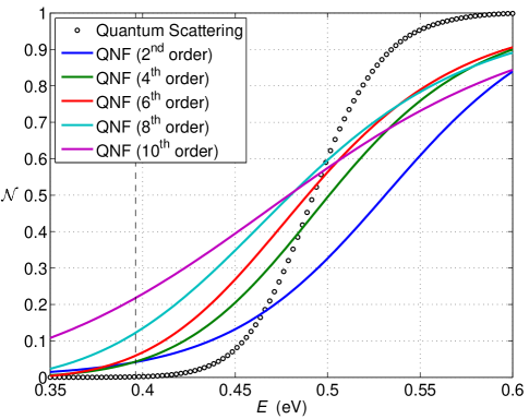
Figure 1: Cumulative reaction probability as a function of the total energy, ${\mathcal{N}}(E)$, for the collinear reaction (37) involving three ¹H atoms. The effective Planck’s constant is $\hbar_{\mathrm{eff}}\approx 3.07\times 10^{-2}$. The vertical dashed line shows the saddle point energy, $E_{0}$, of the PK PES.

Figure 1 shows the CRP, ${\mathcal{N}}(E)$, as a function of the total energy $E$ for a collinear hydrogen, ¹H, exchange reaction, Eq. (37), on the PK PES. The circular points represent ${\mathcal{N}}(E)$ obtained in the reactive quantum scattering calculation, and can, therefore, be regarded as the ‘exact’ CRP values. The vertical dashed line shows the saddle point energy, $E_{0}$, of the PK PES. The five solid colored lines represent the ${\mathcal{N}}(E)$ curves corresponding to different orders, $N=2,4,\ldots,10$, of the QNF computation. As we argue in Sec. IV, one of the sources of the apparent failure of the QNF method to reproduce the correct values of the CPR in the collinear ¹H triatomic system is the very slow convergence (or perhaps even divergence) of the QNF expansion for the value of the effective Planck’s constant, $\hbar_{\mathrm{eff}}\approx 3.07\times 10^{-2}$, characterizing this particular reacting system. Another reason for the QNF theory to be unable to predict correct CPR values for the hydrogen exchange reaction is the importance of the corner cutting tunneling trajectories miller86 in reaction dynamics of light-atom systems. These tunneling trajectories avoid passing through the immediate neighborhood of the saddle-center-…-center equilibrium point in phase space and, therefore, their contribution to the CRP can not be captured by the QNF theory.

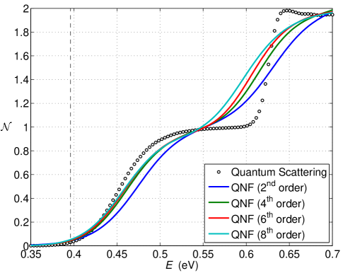
Figure 2: Cumulative reaction probability as a function of the total energy, ${\mathcal{N}}(E)$, for the collinear reaction (37) with ³H (tritium) isotopes of hydrogen. The effective Planck’s constant is $\hbar_{\mathrm{eff}}\approx 1.77\times 10^{-2}$. The vertical dashed line shows the saddle point energy, $E_{0}$, of the PK PES.

Figure 2 presents the CRP-vs-energy curves obtained in the reactive quantum scattering approach (circular points) and by the QNF calculation (colored solid lines) of different orders, $N=2,4,\ldots,8$, for the triatomic collinear system of ³H (tritium) isotopes of hydrogen. The vertical dashed line shows the saddle point energy, $E_{0}$, of the PK PES. The effective Planck’s constant characterizing the system is now $\hbar_{\mathrm{eff}}\approx 1.77\times 10^{-2}$. The convergence of the QNF $\hbar_{\mathrm{eff}}$-expansion, for the energies up to $\sim$0.54 eV, is now evident from the figure. However, the QNF-predicted CRP values approximate the reactive quantum scattering ${\mathcal{N}}(E)$ data only at small energies. As in the case of the ¹H exchange reaction, see fig. 1, we attribute the disagreement of the QNF and reactive quantum scattering CRP values to the non-negligible contributions of tunneling trajectories which avoid passing through the neighborhood of the saddle.

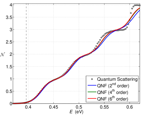
Figure 3: Cumulative reaction probability as a function of the total energy, ${\mathcal{N}}(E)$, for the collinear reaction (37) with hypothetical ²⁰H isotopes of hydrogen. The effective Planck’s constant is $\hbar_{\mathrm{eff}}\approx 6.9\times 10^{-3}$. The ${\mathcal{N}}(E)$ curves obtained with the $4^{\mathrm{th}}$ and $6^{\mathrm{th}}$ order QNF are basically indistinguishable for most of the energy range. The vertical dashed line shows the saddle point energy, $E_{0}$, of the PK PES.

Figure 3 presents the results of the CRP calculations for a collinear system of three hypothetical ²⁰H isotopes of hydrogen. As before, the circular data points correspond to the reactive quantum scattering data and are treated as exact CRP values. The three colored solid lines show the QNF ${\mathcal{N}}(E)$ curves of orders $N=2,4,6$; the ${\mathcal{N}}(E)$ curves obtained with the $4^{\mathrm{th}}$ and $6^{\mathrm{th}}$ order QNF are essentially indistinguishable for most of the energy range. The vertical dashed line shows the saddle point energy, $E_{0}$, of the PK PES. The model system is characterized by $\hbar_{\mathrm{eff}}\approx 6.9\times 10^{-3}$. The convergence of the QNF $\hbar_{\mathrm{eff}}$-expansion, as well as the quantitative agreement of the QNF predictions and exact CPR values for energies $E\lesssim 0.45$ eV, is evident from the figure.

Comparison of figs. 1-3 allows us to conclude that, while basically failing for systems of light atoms, the QNF method of computing the CPR proves very effective for treating heavy-atom reactive systems. On the contrary, the full reactive quantum scattering computations are only feasible for reactive systems consisting of light atoms, and the computations rapidly become formidable as the atomic mass is increased walker .

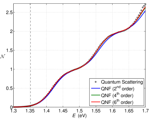
Figure 4: Cumulative reaction probability as a function of the total energy, ${\mathcal{N}}(E)$, for the collinear nitrogen exchange reaction (38). The effective Planck’s constant is $\hbar_{\mathrm{eff}}\approx 8.2\times 10^{-3}$. The ${\mathcal{N}}(E)$ curves obtained with the $4^{\mathrm{th}}$ and $6^{\mathrm{th}}$ order QNF are essentially indistinguishable for most of the energy range. The vertical dashed line shows the saddle point energy, $E_{0}$, of the LEPS PES.

Finally, in order to further illustrate the efficiency of the QNF technique for treating heavy-atom systems we compute the CRP for the collinear nitrogen exchange reaction (38) on the LEPS PES. Figure 4 compares the CRP values obtained in the reactive quantum scattering calculation (circular data points) and those given by the QNF analysis (colored solid lines) of orders $N=2,4,6$. The system is characterized by $\hbar_{\mathrm{eff}}\approx 8.2\times 10^{-3}$. The vertical dashed line shows the saddle point energy, $E_{0}$, of the LEPS PES. The ${\mathcal{N}}(E)$ curves obtained with the $4^{\mathrm{th}}$ and $6^{\mathrm{th}}$ order QNF are essentially indistinguishable for most of the energy range; this fact signals the rapid convergence of the QNF $\hbar_{\mathrm{eff}}$-expansion for the given value of the effective Planck’s constant. The quantitative agreement of the exact and QNF values of ${\mathcal{N}}(E)$ extends up to energies of $\sim$1.5 eV.

The QNF calculation of the CRP requires significantly less computational time than the corresponding full quantum reactive scattering calculation. For example, the 6${}^{\text{th}}$ order QNF computation of the nitrogen-exchange CRP curve in Fig. 4 took about 10 minutes on a 2.6 GHz processor, 2 GB RAM computer, while the corresponding full quantum reactive scattering computation took more than 12 hours on the same machine. The QNF approach becomes even more advantageous for treating chemical systems of atoms heavier than nitrogen: the expense of the full quantum computations rapidly grows with the number of asymptotic channels (and, therefore, with mass) walker , while the QNF expansion only becomes more rapidly convergent making the corresponding analysis computationally cheaper.

IV Convergence of QNF

While it is well known that for $d=2$ degrees of freedom, the classical normal form (CNF) converges in the neighborhood of saddle-center equilibrium points (see, e.g., giorgilli ; moser ) this is not clear for the QNF (for the first results in this direction see anikin ). Still, in the following we provide a qualitative discussion of the convergence of the QNF based on our calculations performed for the triatomic collinear reactions of Sec. III.

The QNF approximates the Hamiltonian of the reaction system in a phase-space vicinity of the saddle-center equilibrium point. Thus, for instance, in computing the CRP one only expects this approximation to render reliable results in a certain energy range around the saddle point energy $E_{0}$ of the PES under consideration. The energy difference $(E-E_{0})$ may therefore be considered as one small parameter in the QNF expansion. The role of the other small parameter is played by the effective Planck’s constant, $\hbar_{\mathrm{eff}}$. It is the convergence of the QNF with respect to this second small parameter that we focus on in this section.

We proceed by considering the right hand side of Eq. (34), i.e., the QNF, at $I=0$, corresponding to no ‘energy’ in the reaction coordinate, and $n_{2}=0$, giving the zero-point ‘vibrational energy’ of the transverse degree of freedom. Then, Eq. (34) becomes

$$E=E_{0}+\sum_{n=1}^{\lfloor N/2\rfloor}c_{n}\hbar_{\mathrm{eff}}^{n}\,.$$ (39)

For the case of the PK PES the first five expansion coefficients are $c_{1}=0.161982$, $c_{2}=1.193254$, $c_{3}=14.90023$, $c_{4}=378.7950$, and $c_{5}=1227.035$. As $N\rightarrow\infty$ the radius of convergence $\hbar_{\mathrm{eff}}^{(0)}$ of the sum in Eq. (39) is given by

$$\hbar_{\mathrm{eff}}^{(0)}=\lim_{n\to\infty}\frac{c_{n}}{c_{n+1}}\,.$$ (40)

Here, we make a crude estimate of $\hbar_{\mathrm{eff}}^{(0)}$ by only considering the first five expansion coefficients in Eq. (40), i.e., $c_{n}$ with $n=1,\ldots,5$; then, the radius of convergence is given by $\hbar_{\mathrm{eff}}^{(0)}\sim 0.04$.

The estimated value of $\hbar_{\mathrm{eff}}^{(0)}$ sheds light on the seeming inefficiency of the QNF theory for CRP computations in light atom reactions. Indeed, the ¹H exchange reaction, see Fig. 1, is characterized by $\hbar_{\mathrm{eff}}=3.07\times 10^{-2}$. This value being close to $\hbar_{\mathrm{eff}}^{(0)}$ signals that the corresponding QNF expansion converges very slowly, if at all, and, possibly, terms of orders far beyond $N=10$ are needed for a reliable CRP prediction in Fig. 1.

In the case of the ³H exchange reaction the effective Planck’s constant is $\hbar_{\mathrm{eff}}=1.77\times 10^{-2}$ and is thus smaller than $\hbar_{\mathrm{eff}}^{(0)}$. This fact is in agreement with the apparent speed-up of the convergence of the CRP values, see Fig. 2, in comparison with the ¹H case. Finally, the convergence is very fast and pronounced for the case of the heavy (hypothetical) ²⁰H atoms, see Fig. 3, for which $\hbar_{\mathrm{eff}}=6.9\times 10^{-3}$ which is much smaller that the estimated convergence radius.

V Conclusions

In this paper we used the quantum normal form (QNF) approach to quantum transition state theory schubert_prl ; wsw08 for computing the cumulative reaction probability for triatomic collinear reactions. The QNF leads to a realization of quantum transition state theory which is very much in the spirit of (classical) transition state theory. Similar to the classical case where a recrossing free dividing surface can be constructed from a classical normal form such that reaction probabilities can be computed from the flux through the dividing surface, the QNF can be viewed to give quantum reaction probabilities as the quantum mechanical flux through the same (classically recrossing free) dividing surface. So unlike reactive scattering techniques which involve full, global quantum computations, the QNF realization of quantum transition state theory requires only local information in the neighborhood of the saddle equilibrium point which governs the reaction. In this paper we demonstrated, that for heavy atom systems (comprised of ten or more nucleons) the QNF this way indeed gives a very efficient method for computing cumulative reaction probabilities. Here we measure ‘efficiency’ by the effort for both implementing and computing the QNF. The latter are both comparable to implementing and computing the classical normal form which lead to the realization of classical transition state theory (in particular for multidimensional systems). The major difference between the classical and quantum case is that the QNF computation involves the Moyal bracket which slightly more complicated (and thus computationally more expensive) than the Poisson bracket in the classical case. Nevertheless the efforts for implementing and computing the QNF are far lower than for the full reactive scattering computations to which we compared our results.

We saw, however, that for reactions involving light reactions (such as the hydrogen exchange reaction) the QNF gave only very poor results. We attributed the failure of the QNF computation in these cases to the presence of corner cutting tunneling trajectories which are not captured by the QNF. This way the QNF and reactive scattering methods can be viewed as complementary methods where the latter gives very good results for light atom systems and the former displays its full power especially for heavy atom systems for which reactive scattering approaches become very difficult or even unfeasible due to the growing number of reactive channels that have to be taken into account walker .

We note that also other approximation techniques such as the initial value representation (IVR) ivr have been shown to be fruitful for reaction probability analysis of collinear triatomic reactions garashchuk . However, in order to properly account for interference effects the IVR method requires propagation of a huge number of classical trajectories and, therefore, can pose difficulties for application to high-dimensional atomic systems whereas the difficulties in computing the QNF do not grow so rapidly with the number of degrees of freedom. In fact it would be very interesting to make a detailed comparison between the QNF and the IVR approach.

Another benefit of the QNF approach to compute cumulative reaction probabilities lies in the fact that it involves only little (local) information of the Born-Oppenheimer PES; namely the Taylor expansion of the PES about the saddle equilibrium point governing the reaction. In fact we saw that highly accurate results over quite a broad energy range can already be obtained from the 4${}^{\text{th}}$ or 6${}^{\text{th}}$ Taylor expansion which enters the QNF of the same order. This is especially useful for systems for which the computation of the global PES required in other methods is very difficult.

VI Acknowledgments

A.G. and H.W. acknowledge support by EPSRC under grant number EP/E024629/1. Part of this work was carried out using the computational facilities of the Advanced Computing Research Centre, University of Bristol. S.W. acknowledges the support of ONR Grant No. N00014-01-1-0769, and also the stimulating environment of the NSF sponsored Institute for Mathematics and its Applications (IMA) at the University of Minnesota, where some of this work was carried out. We are also grateful to Prof. Gregory S. Ezra for reading an earlier version of this manuscript and offering useful comments.

References

- (1) P. Pechukas and F. J. McLafferty, J. Chem. Phys. 58, 1622 (1973).
- (2) P. Pechukas and E. Pollak, J. Chem. Phys. 69, 1218 (1978).
- (3) Wiggins S.: Normally Hyperbolic Invariant Manifolds in Dynamical Systems. Springer: Berlin 1994
- (4) T. Uzer, C. Jaffé, J. Palacián, P. Yanguas, and S. Wiggins, Nonlinearity, 15, 957 (2001).
- (5) H. Waalkens and S. Wiggins, J. Phys. A, 37, L435, (2004).
- (6) R. Schubert, H. Waalkens, and S. Wiggins, Phys. Rev. Lett. 96, 218302 (2006).
- (7) H. Waalkens, R. Schubert, and S. Wiggins, Nonlinearity 21, R1 (2008).
- (8) Miller, W. H.: J. Phys. Chem. A, 102, 793 (1998)
- (9) Miller, W. H.: Spiers Memorial Lecture, Farad. Discuss. 110 1 (1998)
- (10) T. Seideman and W. H. Miller, J. Chem. Phys. 95, 1768 (1991).
- (11) W. H. Miller, J. Phys. Chem. A 102, 793 (1998).
- (12) L. M. Delves, Nucl. Phys. 9, 391 (1959); Nucl. Phys. 20, 275 (1960).
- (13) R. N. Porter and M. Karplus, J. Chem. Phys. 40, 1105 (1964).
- (14) A. Lagana, E. Garcia, and L. Ciccarelli, J. Phys. Chem. 91, 312 (1987).
- (15) G. Hauke, J. Manz, and J. Römelt, J. Chem. Phys. 73, 5040 (1980).
- (16) A. Kuppermann, J. A. Kaye, and J. P. Dwyer, Chem. Phys. Lett. 74, 257 (1980).
- (17) D. E. Manolopoulos and S. K. Gray, J. Chem. Phys. 102, 9214 (1995).
- (18) R. I. McLachlan and P. Atela, Nonlinearity 5, 541 (1991).
- (19) W. H. Miller, Science 233, 171 (1986).
- (20) R. B. Walker and J. C. Light, Ann. Rev. Phys. Chem. 31, 401 (1980).
- (21) A. Giorgilli, Discr. Cont. Dyn. Sys., 7(4), 855 (2001).
- (22) J. Moser, Comm. Pure Appl. Math., 11, 257 (1958).
- (23) A. Anikin, Reg. Chaot. Dyn. 13, 377 (2008).
- (24) W. H. Miller, J. Phys. Chem. A 105, 2942 (2001); Y. Elran and K. G. Kay, J. Chem. Phys. 114, 4362 (2001); J. Chem. Phys 116, 10577 (2002).
- (25) S. Garashchuk, F. Grossmann, and D. Tannor, J. Chem. Soc., Faraday Trans. 93, 781 (1997).