Selectivity in binary fluid mixtures: static and dynamical properties

Abstract

Selectivity of particles in a region of space can be achieved by applying external potentials to influence the particles in that region. We investigate static and dynamical properties of size selectivity in binary fluid mixtures of two particles sizes. We find that by applying an external potential that is attractive to both kinds of particles, due to crowding effects, this can lead to one species of particles being expelled from that region, whilst the other species is attracted into the region where the potential is applied. This selectivity of one species of particle over the other in a localized region of space depends on the density and composition of the fluid mixture. Applying an external potential that repels both kinds of particles leads to selectivity of the opposite species of particles to the selectivity with attractive potentials. We use equilibrium and dynamical density functional theory to describe and understand the static and dynamical properties of this striking phenomenon. Selectivity by some ion-channels is believed to be due to this effect.

I Introduction

Biological ion channels are amazing nanofluidic devices. Ion channels are special proteins with pores through the center that allow for passive transport of ions, such as K⁺ and Na⁺, along their electrochemical gradients, through a membrane formed by a lipid bilayer. The pores of these proteins have a diameter of order a few Ångstroms and, in general, have a charge of their own. Ion channels have two important functions: (i) They can open and close the pore and thereby control the current through the channel. This phenomenon is called gating. (ii) Typically, they can select the type of ions that can pass through the pore, a phenomenon called selectivity. Selectivity can occur with respect to several properties. Some channels can select divalent ions over monovalent ones. Other channels can distinguish ions of the same valency by size. Using gating and selectivity, ion channels are responsible for a wide range of physiological phenomena such as the regulation of ion concentrations inside the cell Hille (2001).

The selectivity with respect to ions of equal electrical charge (e.g., between K⁺ and Na⁺) is rather puzzling. Recent theoretical studies of ion channels with wide pores, such as the l-type Ca channel, examined the effects of entropy (also referred to as molecular crowding) in the three component mixture composed of neutral solvent molecules and two ion species, which differ only in size, and also studied the influence of the electrostatic attraction of the ions into the channel Roth and Gillespie (2005). It was found that the entropic effects can dominate over the electrostatic attractions. The theories used in these studies were (i) equilibrium density functional theory (DFT) for mixtures of hard spheres in an external field and (ii) bulk fluid models of charged hard spheres, in which the external potentials are mapped on to shifts in the chemical potentials of the different components Nonner et al. (2000, 2001); Gillespie et al. (2002).

In recent years, colloidal suspensions have become popular model systems for testing all aspects of liquid state theory, including DFT. In contrast to atomic or molecular fluids, colloidal suspensions can conveniently be studied optically, e.g., by confocal microscopy. In addition, individual or groups of colloids can be manipulated using optics: particles which are optically denser than the surrounding solvent are attracted to regions of higher light intensity, e.g, to a laser focus. This is the working principle of optical tweezers, which allows for the creation of an attractive potential well for the colloids, by means of laser irradiation. Because of this ability to manipulate and observe the individual colloids, we believe that, as has been the case for other liquid state phenomena, colloidal suspensions provide a useful model system in which to understand how selectivity in some ion channels occurs. Thus, although the present study is motivated by the desire to further understand entropy driven selectivity in ion channels, we consider a more general scenario. Using an accurate DFT, we study equilibrium selectivity and using dynamical density functional theory (DDFT) we study the dynamics of selectivity in colloidal binary mixtures.

Dynamical aspects of selectivity have neither been studied experimentally nor theoretically, up to now. While a microscopic dynamical theory for so-called ‘simple’ liquids is still under construction Archer (2006, 2009); Anero and Español (2007); Melchionna and Marconi (2008); Marconi and Melchionna (2009), the DDFT for Brownian particles (i.e. for colloidal suspensions) Marconi and Tarazona (1999, 2000); Archer and Rauscher (2004) has been applied with success to a large number of situations, ranging from phase separation Archer (2005) and spinodal decomposition Archer and Evans (2004) to the micro-rheology of colloid polymer mixtures Rauscher et al. (2007); Gutsche et al. (2008).

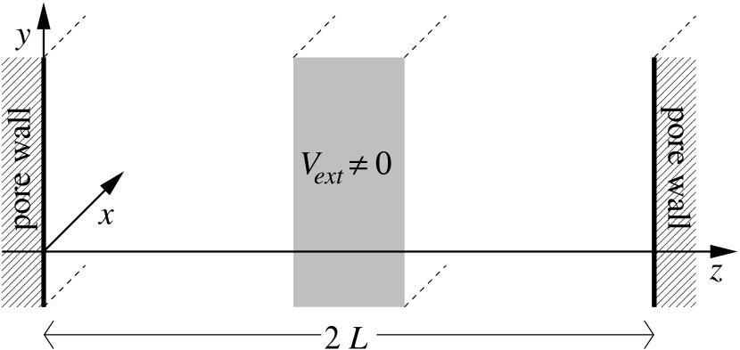
Figure 1: We consider a binary colloidal mixture confined in a three-dimensional slit pore of width $2\,L$. In the center of the slit pore an attractive or repulsive external potential $V_{{ext}}$ acts on the particles. This external potential can lead to selectivity of one species of particle over the other in this region of the slit.

Here, we use DDFT to study the dynamics of selectivity in a binary colloidal mixture of particles of two different sizes. We consider the situation where the mixture is confined within a three-dimensional slit pore, where, apart from the usual fluid ordering near the walls of the slit, the equilibrium fluid is homogeneously distributed within the slit. At time $t=0$, we switch on an external potential in the center of the channel (see Fig. 1) and then follow the time evolution of the system using DDFT. We select this configuration since it may be realized experimentally in a straightforward manner, by using laser tweezers to create the external potentials.

This paper is laid out as follows: In Sec. II we give a short overview of static and dynamical DFT and describe the model system under consideration. Sec. III begins with a discussion of the influence of external potentials on the equilibrium fluid density distributions. This is followed by a discussion of the dynamics of selectivity for a binary mixture of hard spheres. We close with a summary and an outlook in Sec. IV.

II Theory and model system

The theories that we use for describing the fluid are static (equilibrium) DFT and DDFT. Here, we only introduce the aspects of the theories that are relevant to the present study. For a detailed introduction to DFT, see e.g. Refs. Hansen and McDonald (2006); Evans (1992, 1979) and for an introduction to DDFT, see Refs. Marconi and Tarazona (1999, 2000); Archer and Rauscher (2004); Archer and Evans (2004).

II.1 Equilibrium DFT

We consider a fluid mixture composed of $\nu$ different types of particles at a temperature $T$, confined within a fixed volume $\Gamma$. For systems where external potentials $V_{\text{ext}}^{(i)}(\mathbf{r})$ are acting on particles of type $i$, with $i=1\dots\nu$, treating the system in the grand canonical ensemble, one can rigorously prove the existence of the grand potential (free energy) functional $\Omega[\{\rho_{i}\}]$. The set of equilibrium fluid density profiles $\{\rho_{i}^{(\text{eq})}(\mathbf{r})\}$, are those which minimize $\Omega[\{\rho_{i}\}]$. The minimum value of $\Omega[\{\rho_{i}\}]$ is the grand potential of the system Evans (1979). The grand potential functional may be written in the following way:

$$\Omega[\{\rho_{i}\}]=\mathcal{F}[\{\rho_{i}\}]+\sum\limits_{i=1}^{\nu}\int\limits_{\Gamma}\rho_{i}(\mathbf{r})\left[V_{\text{ext}}^{(i)}(\mathbf{r})-\mu_{i}\right]d^{3}r,$$ (1)

where $\mu_{i}$ is the chemical potential for particles of type $i$ and the intrinsic Helmholtz free energy functional

$$\mathcal{F}[\{\rho_{i}\}]=\sum\limits_{i=1}^{\nu}\frac{1}{\beta}\,\int\limits_{\Gamma}\rho_{i}(\mathbf{r})\left[\ln\lambda_{i}^{3}\,\rho_{i}(\mathbf{r})-1\right]d^{3}r+\mathcal{F}_{{ex}}[\{\rho_{i}\}],$$ (2)

which is the sum of the ideal-gas parts, where $1/\beta=k_{B}\,T$ is the thermal energy, $\lambda_{i}$ is the thermal De Broglie wavelength, and $\mathcal{F}_{{ex}}[\{\rho_{i}\}]$ is the free energy contribution originating from the interactions between the particles.

From the minimization principle on $\Omega[\{\rho_{i}\}]$, it follows that the equilibrium fluid density profiles are the solution of the following Euler-Lagrange equations:

$$\frac{\delta\Omega[\{\rho_{i}\}]}{\delta\rho_{i}(\mathbf{r})}=0=\beta^{-1}\ln\lambda_{i}^{3}\rho_{i}(\mathbf{r})+\frac{\delta\mathcal{F}_{{ex}}[\{\rho_{i}\}]}{\delta\rho_{i}(\mathbf{r})}+V_{\text{ext}}^{(i)}(\mathbf{r})-\mu_{i}.$$ (3)

For a given set of external potentials $\{V_{\text{ext}}^{(i)}(\mathbf{r})\}$, these yield a set of non-linear equations for the density profiles $\{\rho_{i}(\mathbf{r})\}$, which can be solved e.g. using an iterative numerical algorithm.

The excess free energy functional $\mathcal{F}_{{ex}}[\{\rho_{i}\}]$ is only known exactly for a few one-dimensional model systems. However, for many experimentally relevant systems, approximate functionals have been constructed which yield results that are in quantitative agreement with experiments and simulations. In particular, this is the case for mixtures of hard spheres, for which functionals arising from fundamental measure theory (FMT), mainly based on geometric considerations, have been developed Rosenfeld (1989); Roth et al. (2002); Hansen-Goos and Roth (2006). In FMT the excess free energy functional is given by

$$\beta{\cal F}_{ex}[\{\rho_{i}\}]=\int\Phi(\{n_{\alpha}(\mathbf{r})\})\,d^{3}r\,,$$ (4)

where the excess free energy density $\Phi$ is a function of a set of weighted densities

$$n_{\alpha}(\mathbf{r})=\sum_{i=1}^{\nu}\int\rho_{i}(\mathbf{r}^{\prime})\,\omega_{\alpha}^{i}(\mathbf{r}-\mathbf{r}^{\prime})\,d^{3}r^{\prime}.$$ (5)

In Eq. (5) the geometrical weight functions are denoted by $\omega_{\alpha}^{i}(\mathbf{r})$ and $\alpha$ labels four scalar and two vector-like weight functions. It is the fundamental measure theory constructed in Ref. Roth et al. (2002) that we implement in this study.

II.2 Dynamical DFT

In a manner analogous to the Runge-Gross theorem for quantum systems Runge and Gross (1984), one can prove the existence of a dynamical density functional theory for classical systems Chan and Finken (2005). As in the static case, the proof of the existence of a DDFT does not lead to having a theory with which one can do calculations. However, for systems of Brownian particles with over-damped stochastic equations of motion [see Eq. (6), below], a successful DDFT has been developed by Marconi and Tarazona Marconi and Tarazona (1999, 2000) for calculating the time evolution of the ensemble average density profiles $\rho_{i}(\mathbf{r},t)$, $i=1\dots\nu$. Note that by ‘ensemble average’ density, we mean an average over the ensemble of different realizations of the stochastic noise terms and particle starting positions in the equations of motion. For a detailed discussion of the differences between the dynamics of the ensemble averaged, the instantaneous, and the coarse grained density, see Ref. Archer and Rauscher (2004).

In real three-dimensional systems, the number of particles in a volume $\Gamma$ can be changed only by a flux through the boundaries $\partial\Gamma$, which, in absence of chemical reactions, directly leads to local particle conservation. In Sec. II.1 above, we discussed DFT, an equilibrium statistical mechanical theory for non-uniform fluid mixtures in the grand canonical ensemble. However, for systems with impermeable boundaries, the equilibrium limit leads to the canonical ensemble. For this reason we consider fixed numbers $N_{i}$ of particles of type $i$ at positions $\mathbf{r}^{(i)}_{n}(t)$, where ${n=1\dots N_{i}}$, and we assume that the particle dynamics is governed by the following over-damped Brownian equations of motion:

$$\frac{d\mathbf{r}^{(i)}_{n}}{dt}=\gamma_{i}\,\left[-\bm{\nabla}V_{\text{ext}}^{(i)}(\mathbf{r}^{(i)}_{n})+\mathbf{F}_{n}^{(i)}\right]+\sqrt{k_{B}\,T\,\gamma_{i}}\,\mathbf{N}_{n}^{(i)}(t),$$ (6)

where $\mathbf{F}_{n}^{(i)}$ is the net force on particle $n$ of type $i$, due to the interactions with all the other particles in the system and $\gamma_{i}$ is the mobility coefficient for particles of type $i$. $\mathbf{N}_{n}^{(i)}$ is a Gaussian random white noise, with zero mean and the correlator

$$\left\langle\mathbf{N}_{n}^{(i)}(t)\circ\mathbf{N}_{m}^{(j)}(t^{\prime})\right\rangle=2\,\delta_{nm}\,\delta_{ij}\,\delta(t-t^{\prime})\,\bm{1}.$$ (7)

The Fokker-Planck equation corresponding to Eq. (6) describes the time evolution of $W(\{\mathbf{r}_{n}^{(i)}\},t)$, the probability of finding the particles in the system at the positions $\mathbf{r}_{n}^{(i)}$ at time $t$. By integrating over $W(\{\mathbf{r}_{n}^{(i)}\},t)$ with respect to all but one of the coordinates of particles of type $i$, one obtains a time evolution equation for the ensemble averaged density $\rho_{i}(\mathbf{r},t)$ Archer (2005). For systems of particles interacting via pairwise interaction potentials, the resulting time evolution equations for $\rho_{i}(\mathbf{r},t)$ depend only on the non-equilibrium two-body distribution functions, but for systems interacting via many-body interaction potentials, the time evolution equations for $\rho_{i}(\mathbf{r},t)$ depend on the higher-body distribution functions Archer and Evans (2004). The time evolution equations for $\rho_{i}(\mathbf{r},t)$ are the lowest members in a hierarchy of $\sum_{i=1}^{\nu}N_{i}$ equations that is similar to the Bogoliubov-Born-Green-Kirkwood-Yvon (BBGKY) hierarchy Archer and Rauscher (2004); Hansen and McDonald (2006); Archer (2005, 2006, 2009). The DDFT is obtained by using a closure relation to truncate the hierarchy. This is done by approximating the non-equilibrium two-body and higher-body distribution functions by the same quantities in an equilibrium system with the same one-body density distributions Marconi and Tarazona (1999, 2000); Archer and Evans (2004). One can show that for a system with a given set of density distributions $\{\rho_{i}(\mathbf{r})\}$, one can find a unique set of external potentials $\{V_{\text{ext}}^{(i)}(\mathbf{r})\}$, such that the system would be at equilibrium if it was exposed to these external potentials. This closure leads to the following set of coupled DDFT equations Archer (2005):

$$\frac{\partial\rho_{i}(\mathbf{r},t)}{\partial t}=\gamma_{i}\,\bm{\nabla}\cdot\left[\rho_{i}(\mathbf{r},t)\,\bm{\nabla}\frac{\delta\Omega[\{\rho_{i}\}]}{\delta\rho_{i}}\right],$$ (8)

where the functional $\Omega[\{\rho_{i}\}]$ is the equilibrium grand potential functional, given in Eq. (1). Note, that the gradient of the variation of the grand potential equals the gradient of the variation of the total free energy, i.e., the sum of the intrinsic free energy $\mathcal{F}[\{\rho_{i}\}]$ and the contributions from the external potentials $V_{{ext}}$. For non-interacting particles, Eq. (8) reduces to the drift-diffusion equation. The (equilibrium) closure approximation used to obtain these equations means that there are some limitations on what kinds of problems the DDFT can be applied to. For example, one can not use it to describe barrier crossing in systems with free energy barriers. However, some aspects of glassy systems can be described within the DDFT framework Archer et al. (2007).

In order to implement Eq. (8) using the FMT approximation for $\Omega[\{\rho_{i}\}]$, we may take advantage of certain simplifications that arise due to the structure of the FMT when calculating the gradient of the variation of the excess free energy. We present this in the Appendix.

II.3 Model system

The model system that we study is a binary mixture of hard-spheres, composed of small ($s$) and big ($b$) particles with sphere radii $R_{s}$ and $R_{b}$, respectively. The particle densities are $\rho_{s}(\mathbf{r},t)$ and $\rho_{b}(\mathbf{r},t)$. We first consider a bulk mixture with given densities and examine the influence of external potentials, which can be either attractive or repulsive, that act on a localized region.

Depending on the origin of the external potentials, they may act in the same way on both types of particles, or alternatively the potentials may be proportional to the volume of the particles. In studies of ion channels with wide selectivity filters with fixed charges, such as the l-type calcium channel, it was found that a competition between energy and entropy can explain size selectivity Nonner et al. (2000, 2001); Gillespie et al. (2002). In such ion-channels the external potentials acting on the ions are generated by the electric field due to the charges fixed in the selectivity filter. Since the potentials generated in this way are the same for particles carrying the same charge, we model these by setting the potentials acting on both species of particles to be equal, i.e. we set $V_{\text{ext}}^{(s)}(\mathbf{r})=V_{\text{ext}}^{(b)}(\mathbf{r})$, to model a mixture with two sizes of particles having the same sign and magnitude charge on them.

However, one may also consider a different situation: that of e.g. optical tweezers applying a force on colloidal particles within a specified region of space. When the forces acting on a colloidal mixture are generated by optical tweezers, then the external potentials acting on the particles are proportional to the volume of the particles. To model this situation, one should set $V_{\text{ext}}^{(s)}(\mathbf{r})=(R_{s}/R_{b})^{3}V_{\text{ext}}^{(b)}(\mathbf{r})$.

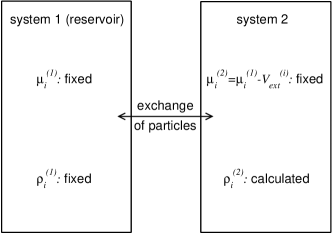
Figure 2: The effect of size selectivity can be rationalized in a simple model of two coupled systems. In system 1, which acts as a reservoir for system 2, the densities of the mixture are fixed to be $\rho_{i}^{(1)}$. In system 2, the chemical potentials are shifted relative to the corresponding values in system 1 by the external potentials $V_{ext}^{(i)}$, which are considered to be constant throughout the system. The different particle densities in system 2 result from these shift in the chemical potentials.

The mechanism of the size selectivity as studied in the next section can be understood by considering a simplified system of a binary colloidal fluid mixture partitioned into two parts: in the first part, a finite region of space, in which the external potentials are applied, and the second part, which acts as a ‘reservoir’, consisting of the remaining parts of the system. If we assume both systems to be infinite in size (i.e., we neglect interface and wall effects) and if we assume $V_{ext}^{(i)}$ to be constant in system 2, we arrive at the situation depicted in Fig. 2 with the chemical potentials $\mu_{i}^{(1)}$ and $\mu_{i}^{(2)}$ in system 1 and 2, respectively given by

$$\mu_{i}^{(\ell)}=\mu_{i}^{(\ell)}(\{\rho_{j}^{(\ell)}\})=\left.\frac{\delta\mathcal{F}}{\delta\rho_{\ell}}\right|_{\left\{\rho_{j}=\rho_{j}^{(\ell)}\right\}}$$ (9)

for $i=s,b$ and $\ell=1,2$ and with the intrinsic free energy $\mathcal{F}[\{\rho_{i}\}]$ defined in Eq. (2). $\rho_{j}^{(\ell)}$ is the spatially constant density of species $j$ in system $\ell$.

In system 1 (which is the reservoir) we specify the densities of the mixture, $\rho_{i}^{(1)}$, where $i=s,b$, which fixes the chemical potentials in system 1. In system 2, which is coupled to system 1, so that particle exchange with the reservoir is allowed, we apply the (spatially constant) external potentials $V_{ext}^{(i)}$. Applying these external potentials is then equivalent to shifts in the chemical potentials in system 2. The densities in system 2, $\rho_{i}^{(2)}$, can thus be computed by solving the following set of equations

$$\mu_{i}^{(1)}(\{\rho_{i}^{(1)}\})=\mu_{i}^{(2)}(\{\rho_{i}^{(2)}\})+V_{ext}^{(i)}\quad\text{for}\quad i=s,b.$$ (10)

If the external potentials are attractive, then the chemical potentials in system 2 are effectively increased over those in system 1, while they are decreased in the case of repulsive potentials. In the low density limit, the Eqs. (10) for $i=s$ and $i=b$ decouple into a pair of independent equations. At higher densities, Eqs. (10) form a non-linear pair of coupled equations for the densities in system 2. As discussed in Sec. IV below, these equations allow us to understand the phenomena described in the next section.

III Results

III.1 The external potentials

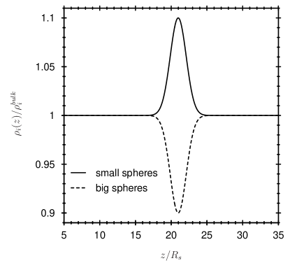
Figure 3: Density profiles $\rho_{i}(z)$, where $i=s,b$, divided by the respective bulk densities $\rho_{i}^{bulk}$ (corresponding to the bulk packing fraction $\eta_{i}=\frac{4}{3}\,R_{i}^{3}\,\pi\,\rho_{i}^{bulk}$), of a binary mixture of hard spheres with a size ratio of $R_{b}=2R_{s}$. The density profiles show small-particle selectivity: locally, with the help of the external potentials, the density of the small spheres (solid line) is slightly increased, while the density of the big spheres (dashed line) is slightly decreased. Using Eq. (11), it is possible to calculate the external potentials $V_{ext}^{i}(z)$, $i=s,b$, which give rise to these equilibrium density profiles. These external potentials are displayed in Fig. 4, for various bulk packing fractions.

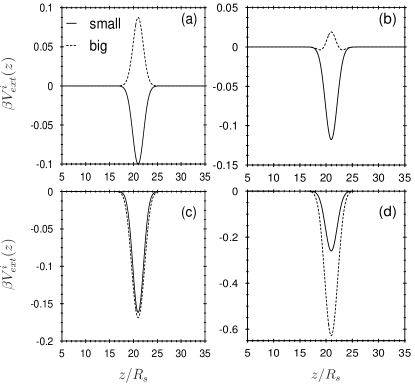
Figure 4: In order to generate a slight local increase in the density of the small spheres and a slight decrease in the density of the big spheres (as displayed in Fig. 3), it is necessary to apply external potentials $V_{ext}^{i}(z)$. Four examples are displayed here for a binary mixture with size ratio $R_{b}=2R_{s}$ and equal bulk packing fractions $\eta_{s}=\eta_{b}$. At low bulk packing fractions $\eta_{s}=\eta_{b}=0.01$, we see in (a) that an attractive potential has to act on the small spheres and a repulsive potential on the big spheres, in order to generate local small-particle selectivity. This can be understood from the ideal-gas limit. In (b), where $\eta_{s}=\eta_{b}=0.04$, the repulsion acting on the big spheres is significantly reduced, as a result of the competition between entropy and energy. In (c), where $\eta_{s}=\eta_{b}=0.09$, both external potentials are roughly the same and are attractive and in (d), where $\eta_{s}=\eta_{b}=0.15$, the attraction required to attract the small particles is weaker than the attraction required to effectively repel the big particles.

Within the framework of static DFT, the equilibrium thermodynamic properties of the system are obtained from the solution of the Euler-Lagrange equations (3), obtained by minimizing the functional in Eq. (1). Typically, one specifies the external potentials $V_{\text{ext}}^{(i)}(\mathbf{r})$ and then computes the resulting equilibrium density distributions $\rho_{i}(\mathbf{r})$, $i=1,\dots,\nu$. However, it is also possible to employ the Euler-Lagrange equations (3) in order to compute the external potentials that give rise to a specified set of density distributions $\{\rho_{i}(\mathbf{r})\}$ Henderson (1991). One obtains:

$$V_{\text{ext}}^{(i)}(\mathbf{r})=-\frac{\delta\mathcal{F}_{{ex}}[\{\rho_{i}\}]}{\delta\rho_{i}(\mathbf{r})}-\beta^{-1}\ln\lambda_{i}^{3}\rho_{i}(\mathbf{r})+\mu_{i}.$$ (11)

It is worth noting that in the limit of vanishing densities, the contribution due to particle interactions, which depends on the variation of $\mathcal{F}_{{ex}}[\{\rho_{i}\}]$, becomes negligible and one recovers the ideal-gas result: $V_{\text{ext}}^{(i)}(\mathbf{r})=-\beta^{-1}\ln\lambda_{i}^{3}\rho_{i}(\mathbf{r})+\mu_{i}$. In the ideal-gas limit, where the density distributions are simply the Boltzmann factors of the external potentials, it is clear that in order to locally increase the density of the particles over the bulk value, attractive potentials are required, and to locally decrease the density, repulsive potentials are needed.

For a one-component interacting system, the behavior is similar to the ideal-gas case, although the density distribution is not simply the Boltzmann factor of the external potential. The density can locally be increased or decreased by an attractive or repulsive external potential, respectively.

The situation becomes more interesting in the case of a binary mixture. If we start with constant densities in an infinite bulk system and wish to generate a set of density profiles such as those shown in Fig. 3, which show a local increase in the density of the small spheres and at the same location a decrease in the density of the big spheres, we can use Eq. (11) to calculate the external potentials required to achieve this.

In Fig. 4 we display the external potentials that one must exert on the system in order to observe the two density profiles shown in Fig. 3, for a binary hard-sphere mixture with $R_{b}=2R_{s}$ and equal bulk packing fractions of the small and large particles, $\eta_{s}$ and $\eta_{b}$, respectively ($\eta_{i}=\frac{4}{3}\,R_{i}^{3}\,\pi\,\rho_{i}^{bulk}$, where $\rho_{i}^{bulk}$ is the density of species $i$ in the bulk, at points in space a large distance from the support of the external potential). At low values of $\eta_{s}=\eta_{b}=0.01$, we see in Fig. 4(a), that the required external potentials are similar to those predicted by the ideal-gas functional. The external potential that gives rise to a local increase in the density of the small spheres is attractive (solid line) and the external potential that gives rise to a decreased in the density of the big spheres is repulsive (dashed line). However, if the bulk packing fractions increase to $\eta_{s}=\eta_{b}=0.04$, as shown in Fig. 4(b), we find that the external potential acting on the big particles is significantly less repulsive than in the low density case displayed in Fig. 4(a). This stems from the competition between energy, due to the interactions of the particles with the external potentials, and entropy, due to the inter-particle interactions and the resulting excluded volume. The influence of the competition between energy and entropy is more pronounced if we increase the bulk packing fractions even further. For $\eta_{s}=\eta_{b}=0.09$, in Fig. 4(c) we see that both species of particles have to be subjected to an attractive potential well, in order to obtain density profiles that locally have an increase in the density of the small particles, at the same time as a decrease in the density of the big particles. For this particular choice of packing fractions, the external potentials for both sizes of particles are roughly the same. In order keep the reduction of the density of the large particles at the same moderate level at much higher packing fractions $\eta_{s}=\eta_{b}=0.15$, the attraction on the big particles has to be much stronger than the attraction on the small particles.

III.2 Equilibrium DFT for selectivity

Figure 5: The external potential acting on the small spheres (solid lines) and big spheres (dashed lines). In addition to the soft slit potentials, we perturb the density distributions by additional potentials in the middle of the slit, which can be either (a) attractive or (b) repulsive.

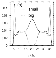
Figure 6: (a) The equilibrium density profiles of a binary hard-sphere mixture with $R_{b}=2\,R_{s}$ confined within a slit with potentials given by Eq. (12). (b) When the attractive potentials in the middle of the slit are switched on [see Fig. 5(a) and Eq. (13)], the density of the small spheres is locally enhanced in the middle of the slit while the density of the big spheres is decreased. This is an example of small particle selectivity. In both (a) and (b) the chemical potentials $\mu_{b}$ and $\mu_{s}$ are chosen such that the adsorptions given by Eq. (14) are $\Upsilon_{b}R_{b}^{2}=0.495$ and $\Upsilon_{s}R_{s}^{2}=1.308$. The chemical potentials in (b) correspond to reservoir packing fractions $\eta_{a}=\eta_{s}=0.15$, as indicated by the dotted line.

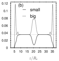
Figure 7: Same as Fig. 6, but for repulsive potentials. (a) The equilibrium density profiles with $R_{b}=2\,R_{s}$ confined within a slit with potentials given by Eq. (12). (b) When the repulsive potentials in the middle of the slit are switched on [see Fig. 5(b) and Eq. (13)], the density of the small spheres is locally reduced in the middle of the slit while the density of the big spheres is increased. This is an example of large particle selectivity. In both (a) and (b) the adsorptions given by Eq. (14) are $\Upsilon_{b}R_{b}^{2}=0.786$ and $\Upsilon_{s}R_{s}^{2}=0.905$. The chemical potentials in (b) correspond to bulk reservoir fractions $\eta_{a}=\eta_{s}=0.15$, as indicated by the dotted line.

From the results presented so far, we can see that the competition between energy and entropy in mixtures can lead to surprising effects. The question that arises is whether or not it is possible to use this competition in order to select one species over the other with the aid of an appropriately chosen external potential. To this end, we consider a binary hard-sphere mixture confined between two planar walls – i.e. in a slit. We model the potentials due to the walls of the slit as follows:

$$V_{\text{ext}}^{(i)}(z)=A\left(\frac{z-z_{0}}{L_{i}}\right)^{m},$$ (12)

where $A=10\,k_{B}\,T$, $z_{0}=20.48\,R_{s}$, $m=20$ and $L_{i}=L+R_{i}$, where $L=15\,R_{s}$. Due to the large value of the power $m$, Eq. (12) models the continuous potentials of a pair of slightly soft parallel planar walls, separated a distance $2\,L$. $z_{0}$ is the center of the slit pore. When the fluid mixture in the slit is at equilibrium, we perturb the fluid by introducing additional external potentials in the middle of the slit, so that the external potentials are:

$$V_{\text{ext}}^{(i)}(z)=A\left(\frac{z-z_{0}}{L_{i}}\right)^{m}+\epsilon_{i}\exp\left[\left(\frac{z-z_{0}}{w}\right)^{2}\right].$$ (13)

The additional second term in the external potentials can be either attractive ($\epsilon_{i}<0$), as shown in Fig. 5(a), or repulsive ($\epsilon_{i}>0$), as indicated in Fig. 5(b). The range of the external potential is $w=3\,R_{s}$ and the depth or height $\epsilon_{i}=\pm 2\,k_{B}\,T$.

First, we consider the case of an attractive potential in the middle of the slit ($\epsilon_{i}<0$). We compare two equilibrium states: (i) the binary mixture in the slit without the additional potentials ($\epsilon_{i}=0$), and (ii) the equilibrium state of the binary mixture with the potentials ($\epsilon_{i}=-2k_{B}T$), shown in Fig. 5(a). We calculate the density profiles which minimize the equilibrium DFT by solving the Euler-Lagrange equations, Eq. (3). Since equilibrium DFT is defined in the grand canonical ensemble, particle exchange between the system and a reservoir, which sets the chemical potentials, is possible. However, we wish to compare our equilibrium DFT calculations with DDFT computations, which preserves the number of particles. In order to make an honest comparison, we minimize the equilibrium DFT under the constraint that the amount of material within the slit is fixed, i.e., that the adsorptions

$$\Upsilon_{i}=\int_{-\infty}^{\infty}\rho_{i}(z)dz,$$ (14)

are fixed. To enforce these constraints, we treat the chemical potentials $\mu_{a}$ and $\mu_{b}$ as Lagrange multipliers and we choose them such that in the case when the potentials in the middle of the slit are switched on, the reservoir packing fractions are $\eta_{s}=\eta_{b}=0.15$. In the case of an attractive potential this results in $\Upsilon_{s}R_{s}^{2}=1.308$ and $\Upsilon_{b}R_{b}^{2}=0.495$, while in the repulsive case the corresponding adsorptions are $\Upsilon_{s}R_{s}^{2}=0.905$ and $\Upsilon_{b}R_{b}^{2}=0.786$. Correspondingly, the reservoir packing fractions when the potentials are switched off are different.

When the attractive potential wells are not switched on, we find that the density profile of the big spheres close to the walls of the slit possess prominent peaks [see Fig. 6(a)], indicating strong packing and correlation effects at the walls of the slit. The density of the small spheres is slightly decreased at the wall. In the middle of the slit we find a region where both densities are constant. When the attractive potentials in the center of the slit are switched on, so that both the small and the big particles are subjected to the external potentials shown in Fig. 5(a), we find that there is a significant local increase in the density of the small particles in the region of the attraction, while the density of the big particles is strongly decreased here – see Fig. 6(b). Hence, if the bulk densities of the big and the small particles are sufficiently large, an attractive potential well can be small particle selective due to the competition between energy and entropy.

We now turn our attention to the case when a repulsive potential is turned on in the middle of the slit – see Fig. 5(b). In Fig. 7(a) we display the equilibrium density profiles for the case when the repulsive potentials are not switched on. The profiles are similar to those shown in Fig. 6(a). The difference is due to our treatment of the chemical potentials as Lagrange multipliers to set the adsorptions in Eq. (14), for the case when the potentials in the middle of the slit are switched on. This leads to the adsorptions and therefore also to the density profiles being different in the two cases when the potentials are switched off.

In Fig. 7(b) we display the equilibrium fluid density profiles for the case when the repulsive potentials in the middle of the slit, for both components, are switched on. In the region where the repulsive external potentials are applied, the local density of the small spheres is decreased and the density of the big spheres is increased. It is interesting to note that despite the repulsion acting on the big particles, the local density of the big spheres is greater than the density in the surrounding fluid. This is an example of big-particle selectivity.

III.3 Dynamics of selectivity

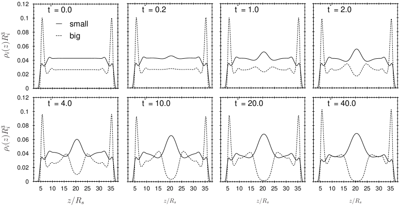
Figure 8: Time evolution of the density profiles of the small (solid lines) and big (dashed lines) spheres from the initial state in Fig. 6(a) towards the final state in Fig. 6(b). At time $t^{*}=0$ we switch on the attractive potentials in the middle of the slit. Note that for short times, both species of particles follow the attraction and move towards the center. However, for larger times $t^{*}>1$, only the density of the small spheres increases in the region of the potential well, while the big spheres move away from the center, despite the attractive external potential.

Figure 9: Time evolution of the density profiles of the small (solid lines) and big (dashed lines) spheres from the initial state in Fig. 7(a) towards the final state in in Fig. 7(b). At time $t^{*}=0$ we switch on the repulsive potentials in the center of the slit. Note that for short times, both species of particles follow the repulsion and move away from the center. However, for larger times $t^{*}>1$, only the density of the small spheres decreases in central region, while the density of the big spheres increases in the center, despite the repulsive external potential.

In order to better understand the behavior of the system, we study the time evolution of the density profiles of both types of particles as they evolve between the two equilibrium states shown in Fig. 6, the case with the attractive potentials applied in the center of the slit, and those shown in Fig. 7, the case where the repulsive potentials are exerted in the center of the slit. In what follows, all times $t^{*}\equiv t/\tau$ are given in units of the Brownian time-scale $\tau=(\beta/\gamma)R_{s}^{2}$; it is roughly the time it takes for a particle to diffuse over a distance equal to its own radius. Note also that we have set the two mobility coefficients to be equal, $\gamma_{1}=\gamma_{2}=\gamma$. In a colloidal suspension this would not be the case: the mobility of spherical particles in a suspension decreases with the inverse of the cross-sectional area. For the systems under consideration here this results in $\gamma_{s}/\gamma_{b}=4$. With the small particles being considerably faster than the big ones, the initial behavior of the big particles described in the following might not be observable in colloidal suspension.

The initial conditions for attractive and repulsive potentials in the center of the slit pore are those displayed in Figs. 6(a) and 7(a), respectively.

In the first case, when we switch on the attractive potentials in the center of the slit at time $t^{*}=0$, initially both types of particles behave as one would intuitively expect: they follow the attraction and move towards the center of the slit. However, this is only the case for short times. This initial influx of particles results in a slight increase in the particle densities at the center of the slit, as can be seen in the density profiles shown in Fig. 8. For times $t^{*}>1$, the drift diffusion behavior of the system qualitatively changes, as the competition between the energy due to the interactions of the spheres with the external potentials and the entropy due to the hard-sphere interactions between particles, sets in. For times $t^{*}>1$, only the small particles follow the attraction and the number density of the small particles in the center of the slit increases further, while the big spheres are expelled from this region. At short times, only spheres in the center of the slit show a net movement and the density profiles do not change over time in the vicinity of the slit walls. However, at longer times, there is a net flux of the small particles from the walls of the slit towards the center and there is also a net flux of big particles from the center towards the walls. This diffusion process is slow and the time it takes for the system to reach the final equilibrium state depicted in Fig. 6(b) is rather long. It also depends on the system size – the wider the slit, the longer it takes for the particles to diffuse (say) from the wall to the center.

We observe similar behavior in the case when we apply repulsive potentials at the center of the slit. When we switch on the repulsive potentials at $t^{*}=0$, both types of particles behave as our intuition suggests, and they follow the repulsion and move way from the center of the slit. This initial flow results in a slight decrease in the particle densities at the center of the slit, as can be seen in the density profiles shown in Fig. 9. However, for longer times $t^{*}>1$, the behavior of the system qualitatively changes, as the competition between the energy and the entropy sets in. For times $t^{*}>1$, only the small particles follow the repulsion and the number density of the small particles in the center of the slit decreases further, while the big spheres become effectively attracted towards this region, and the density of the big particles increases at the center of the slit. The final equilibrium state the one shown in Fig. 7(b).

Note that these counterintuitive results occur only when the densities of the particles are high enough. At low densities, when the system can be modelled as an ideal-gas, attractive potentials always lead to an increase in the densities of both types of particles and repulsive potentials always lead to a decrease.

IV Discussion

Using the bulk approach depicted in Fig. 2 and expressed in Eqs. (10) it is possible to understand the results presented in Sec. III. If the external potentials $V_{ext}^{(i)}$ are the same for all components of the mixture, as assumed in our DFT and DDFT calculations, we can reproduce the increase or decrease of the particle densities in the region where the external potentials are applied: for a binary mixture with size ratio $R_{b}=2\,R_{s}$ and bulk packing fractions of $\eta_{s}=\eta_{b}=0.15$ in the reservoir system 1 (corresponding to $\rho_{s}^{(1)}\,R_{s}^{3}=\rho_{b}^{(1)}\,R_{b}^{3}=0.036$) and an attractive external potential of magnitude $2\,k_{B}\,T$, the density of the small particles in system 2 increases by a factor of 1.91, while the density of the big particles is reduced to 0.008 of its original value. This is in good agreement with the results displayed in Fig. 6: the density of the big particles at the center of the slit pore is negligibly small while the density of the small particles at the same spot is about twice the reservoir density. In the case of a repulsive potential of magnitude $2\,k_{B}\,T$, the density of the big particles increases by a factor of 2.25, while the density of the small spheres is reduced to 0.21 of its value without the field. Again, this agrees rather well with the results shown in Fig. 7.

While we have shown results for size selectivity only for one size ratio, i.e. $R_{b}=2\,R_{s}$, we have confirmed that a binary mixture with less asymmetric radii shows analogous behavior. However, in the case of a less asymmetric size ratio, the amplitude of the attractive or repulsive potential has to be larger to generate a degree of size selectivity similar to that reported in our study.

In addition, Eqs. (10) allows one to easily estimate the influence of the external potentials in other scenarios and determine at what densities the system should or should not display selectivity. For example, if the external potentials are proportional to the volume of the particles, which would be the case in an experimental realization using laser tweezers, then one should expect results similar to those reported here, for a binary mixture with a size ratio $R_{b}=2\,R_{s}$ and packing fractions $\eta_{s}=0.15$ and $\eta_{b}=0.02$. In this case, external fields on the order of $V_{ext}^{(s)}=\pm 1k_{B}T$ and $V_{ext}^{(b)}=\pm 8k_{B}T$ are sufficient to generate selectivity.

In the present study, the relatively wide slit geometry has only a small effect on the selectivity observed. However, for more narrow pores, the grand canonical calculations in a cylindrical channel geometry in Ref. Roth and Gillespie (2005) showed that the confinement can enhance the selectivity.

The arguments presented above are based purely on the equilibrium free energy and hold for any type of underlying dynamics, i.e., for the overdamped Brownian dynamics considered here as well as for systems following Hamiltonian dynamics. A key feature of the dynamics of separation presented in Figs. 8 and 9 is that the big particles, although they are finally driven out of the region in which the attractive potential acts and into the region in which the repulsive potential acts, initially follow the direction given by the gradient of the external potential. For Figs. 8 and 9 we assumed equal mobilities for the big and the small particles. In a colloidal suspension this is not be the case (the mobility of spherical particles in a suspension decreases with the inverse of the cross-sectional area) and so the initial behaviour of the big particles described above might not be observable in a colloidal suspension.

To conclude, we should remind the reader that the DDFT in Eq. (8) that we have used to describe the system, does not incorporate hydrodynamic interactions between the colloidal particles. Whilst hydrodynamic interactions do not affect the static properties of the system (i.e. the equilibrium DFT is still applicable), hydrodynamic interactions do have an influence on the dynamical properties of the system. The influence of hydrodynamic interactions between the particles has been incorporated in the DDFT in several ways Royall et al. (2007); Rex and Löwen (2009). We believe that extending the present study to include the influence of hydrodynamic interactions would not qualitatively change any of the results that we observe since these only influence the dynamics but not the energetics of the system. It is the energetics which determine the final equilibrium state, i.e. whether selectivity can be observed or not.

*

Appendix A DDFT and the Structure of FMT

For the calculation of the time evolution of the density profiles, the gradient of $\delta\Omega/\delta\rho_{i}({\bf r})$ are required in Eq. (8). This includes the gradient of the variation of the excess free energy functional ${\cal F}_{ex}$. Since we employ FMT for the excess free energy, we can make use of the the structure of ${\cal F}_{ex}$, given in Eqs. (4) and (5). Note that in the general, three-dimensional case, the variation of the excess free energy with respect to the density profile of component $i$ can be written as

$$\frac{\delta{\cal F}_{ex}}{\delta\rho_{i}({\bf r})} = \sum_{\alpha}\int\left.\frac{\partial\Phi}{\partial n_{\alpha}}\right|_{{\bf r}^{\prime}}\frac{\delta n_{\alpha}({\bf r}^{\prime})}{\delta\rho_{i}({\bf r})}~{}d^{3}r^{\prime}$$ (15)

$$= \sum_{\alpha}\int\left.\frac{\partial\Phi}{\partial n_{\alpha}}\right|_{{\bf r}^{\prime}}\omega_{\alpha}^{i}({\bf r}^{\prime}-{\bf r})~{}d^{3}r^{\prime}.$$

It follows from Eq. (15) that the gradient acts solely on the weight functions:

$$\bm{\nabla}\frac{\delta{\cal F}_{ex}}{\delta\rho_{i}({\bf r})}=\sum_{\alpha}\int\left.\frac{\partial\Phi}{\partial n_{\alpha}}\right|_{{\bf r}^{\prime}}\bm{\nabla}\omega_{\alpha}^{i}({\bf r}^{\prime}-{\bf r})~{}d^{3}r^{\prime}.$$ (16)

Although the sum in Eqs. (15) and (16) is over four scalar ($\alpha=3,\dots,0$) and two vector-like ($\alpha=v2,v1$) weight functions, one can exploit the relations between the scalar weight functions $4\pi R_{i}^{2}~{}\omega_{0}^{i}=4\pi R_{i}~{}\omega_{1}^{i}=\omega_{2}^{i}$ and the vector-weighted functions $4\pi R_{i}~{}\omega_{v1}^{i}=\omega_{v2}^{i}$. This allows one to reduce to the sum in Eqs. (15) and (16) to three terms by introducing the auxiliary functions

$$\Psi_{3}^{(i)}({\bf r})=\frac{\partial\Phi}{\partial n_{3}},$$ (17)

$$\Psi_{2}^{(i)}({\bf r})=\frac{\partial\Phi}{\partial n_{2}}+\frac{1}{4\pi R_{i}}\frac{\partial\Phi}{\partial n_{1}}+\frac{1}{4\pi R_{i}^{2}}\frac{\partial\Phi}{\partial n_{0}},$$ (18)

and

$$\Psi_{v2}^{(i)}({\bf r})=\frac{\partial\Phi}{\partial n_{v2}}+\frac{1}{4\pi R_{i}}\frac{\partial\Phi}{\partial n_{v1}}.$$ (19)

These functions depend on the particular version of FMT employed. Here we use the White-Bear version Roth et al. (2002).

The slit geometry that we consider in the present study allows us to further simplify the gradient in Eq. (16). The effective one-dimensional weight functions and their derivatives with respect to $z$ are easily calculated. For the volume weight function we find

$$\omega_{3}^{i}(z)=\pi(R_{i}^{2}-z^{2})~{}\Theta(R_{i}-|z|),$$ (20)

where $\Theta(z)$ denotes the Heaviside step-function. The derivative of the volume weight function is

$$W_{3}^{i}(z)=\frac{\partial}{\partial z}\omega_{3}^{i}(z)=-2\pi z~{}\Theta(R_{i}-|z|).$$ (21)

Note that the derivative of the Heaviside function can be neglected, because the weight function $\omega_{3}^{i}(z)$ vanishes at the integration boundaries. The effective surface weight function is

$$\omega_{2}^{i}(z)=2\pi R_{i}~{}\Theta(R_{i}-|z|),$$ (22)

which is constant in the range of integration, so that its derivative

$$W_{2}^{i}(z)=\frac{\partial}{\partial z}\omega_{2}^{i}(z)=2\pi R_{i}~{}\left[\delta(z+R_{i})-\delta(z-R_{i})\right]$$ (23)

has contributions only from the derivative of the Heaviside-$\Theta$ function. Finally, the vector-like weight function is

$$\omega_{v2}^{i}(z)=-2\pi z~{}\Theta(R_{i}-|z|)~{}{\bf e}_{z},$$ (24)

and leads to a derivative

$$W_{v2}^{i}(z) = \frac{\partial}{\partial z}\omega_{v2}^{i}(z)=\left\{-2\pi~{}\Theta(R_{i}-|z|)\right.$$

$$+ \left.2\pi R_{i}~{}\left[\delta(z+R_{i})+\delta(z-R_{i})\right]\right\}~{}{\bf e}_{z}.$$

Putting all the ingredients together we obtain the following expression for the gradient of the variation of the excess free energy in planar geometry:

$$\frac{\partial}{\partial z}\frac{\delta{\cal F}_{ex}}{\delta\rho_{i}(z)} = \int\left\{\Psi_{3}^{(i)}(z^{\prime})~{}W_{3}^{i}(z^{\prime}-z)\right.$$ (26)

$$+ \left.\Psi_{v2}^{(i)}(z^{\prime})~{}W_{v2}^{i}(z^{\prime}-z)\right\}~{}dz^{\prime}$$

$$+ 2\pi R_{i}\left\{\Psi_{2}^{(i)}(z+R_{i})-\Psi_{2}^{(i)}(z-R_{i})\right.$$

$$+ \left.\Psi_{v2}^{(i)}(z+R_{i})+\Psi_{v2}^{(i)}(z-R_{i})\right\}.$$