Level Crossing Rate and Average Fade Duration
of EGC Systems with Cochannel Interference
in Rayleigh Fading

Abstract

Both the first-order signal statistics (e.g. the outage probability) and the second-order signal statistics (e.g. the average level crossing rate, LCR, and the average fade duration, AFD) are important design criteria and performance measures for the wireless communication systems, including the equal gain combining (EGC) systems in presence of the cochannel interference (CCI). Although the analytical expressions for the outage probability of the coherent EGC systems exposed to CCI and various fading channels are already known, the respective ones for the average LCR and the AFD are not available in the literature. This paper presents such analytical expressions for the Rayleigh fading channel, which are obtained by utilizing a novel analytical approach that does not require the explicit expression for the joint PDF of the instantaneous output signal-to-interference ratio (SIR) and its time derivative. Applying the characteristic function method and the Beaulieu series, we determined the average LCR and the AFD at the output of an interference-limited EGC system with an arbitrary diversity order and an arbitrary number of cochannel interferers in forms of an infinite integral and an infinite series. For the dual diversity case, the respective expressions are derived in closed forms in terms of the gamma and the beta functions.

I Introduction

Equal gain combining (EGC) is an important diversity technique that is often used to mitigate fading in various wireless communications systems [1]. The EGC has several practical advantages over other diversity techniques, because it has close to optimal performance and yet is simple to implement. The outage probability (OP) is the primary performances measure for all diversity systems, particularly those exposed to cochannel interference (CCI) such as the cellular mobile systems. When the CCI is the predominant noise source at the receiver, its OP represents the first-order statistical property of the output signal-to-interference ratio (SIR). The OP of the interference-limited EGC systems was studied in [2]-[3] and references therein. Apart from the OP, some aspects in the design and the analysis of wireless communication systems must also consider the signal correlation properties, thus necessitating the determination of its second-order statistical properties: the average level crossing rate (LCR) and the average fade duration (AFD). They are used for proper selection of adaptive symbol rates, interleaver depth, packet length and time slot duration in various wireless communication systems. While these statistics have already been determined for the signal envelope at the output of EGC systems exposed to various fading channels and thermal noise [4]-[6], the SIR statistics of the EGC systems subject to CCI have not yet been derived analytically to the best of author’s knowledge. The average LCR and the AFD of the SIR at the output of selection combining (SC) and maximal-ratio combining (MRC) systems exposed to CCI and various fading (Rayleigh, Rice and Nakagami) channels have been reported only recently in [7]-[8], but these works do not consider the EGC systems. This paper focuses specifically on an interference-limited coherent EGC system with an arbitrary diversity order and an arbitrary number of cochannel interferers, and derives analytical solutions for the average LCR and the AFD of the output SIR in Rayleigh fading channels.

Section II presents the coherent EGC system model and the channel model, including the two feasible scenarios for interference combining. Section III presents the analysis that yields to the analytical solutions of the OP, the average LCR and the AFD in forms of an infinite integral and an infinite series. The Section IV compares the computational burden between these two solutions and provides several numerical examples that illustrate the behaviors of the first-order and the second-order signal statistics. Section V summarizes the main results and concludes the paper.

II System and Channel Models

We consider a coherent EGC communication receiver with $M$ diversity branches. It is exposed to the transmissions of a single desired and $N$ interference users, whose signal replicas in each diversity branch are received over independent identically distributed (IID) Rayleigh flat fading channels.

In each diversity branch $k$ $\>(1\leq k\leq M)$, the desired signal is assumed to have an average power $\Omega_{\rm S}$, while all interference signals have an equal average power $\Omega_{\rm I}$. Thus, the channel gains in each branch can be represented as equivalent complex zero-mean Gaussian random variables (RVs) $W_{i,k}$; more particulary, $W_{0,k}=X_{0,k}\>e^{j\theta_{0,k}}$ with variance $\Omega_{\rm S}$ represents the desired signal in branch $k$, while $W_{i,k}=Y_{i,k}\>e^{j\theta_{i,k}}$ $(1\leq i\leq N)$ with variance $\Omega_{\rm I}$ represents $i$-th interference signal in branch $k$. The phases of the desired signals $\theta_{0,k}$ and the interference signal $\theta_{i,k}$ follow the uniform probability distribution function (PDF) over $[0,2\pi)$, while the respective envelopes $X_{0,k}=\sqrt{|{W_{0,k}|^{2}}}$ and $Y_{i,k}=\sqrt{|{W_{i,k}|^{2}}}$ follow the Rayleigh PDF.

Due to the transmitter/receiver mobility and their relative velocity, the fading channel introduces time correlation of the real and imaginary parts of $W_{0,k}$ (i.e., in-phase and quadrature components of the desired signal) with maximum Doppler frequency shift $f_{m0}$ in their power spectra. Additionally, the real and imaginary parts of the channel gains $W_{i,k}$ of each interfering signal $i$ are also assumed be time correlated with an identical maximum Doppler frequency shift $f_{mi}$.

In EGC systems, the desired signal replicas in each of the $M$ branches are co-phased, equally weighted, and then coherently added to give the resultant desired output signal. For the interference combining, there are two possible scenarios: the signal replicas originating from any interferer can combine either incoherently [2, Section III] or coherently [3].

II-A Incoherent Interference Combining

If the interference signals are combined incoherently at the EGC output, the instantaneous SIR $Z_{1}$ is determined as [2, Eq. (9)],

$$Z_{1}=\frac{(\sum_{k=1}^{M}X_{0,k})^{2}}{\sum_{i=1}^{N}\sum_{k=1}^{M}Y_{i,k}^{2}}\,,$$ (1)

where the powers (i.e. the squared envelopes) of all interference signals in all diversity branches are added together. Thus, any single element in the denominator of (1), $Y_{i,k}^{2}$, is a chi-squared RV with 2 degrees of freedom, so the entire denominator, given by

$$Y_{1}^{2}=\sum_{i=1}^{N}\sum_{k=1}^{M}Y_{i,k}^{2}\,,$$ (2)

follows the chi-squared PDF with $2MN$ degrees of freedom,

$$f_{Y_{1}^{2}}(y)=\frac{1}{(\Omega_{\rm I})^{MN}}\frac{y^{MN-1}}{\Gamma(MN)}\exp\left(-\frac{y}{\Omega_{\rm I}}\right)\,,$$ (3)

where $\Gamma(\cdot)$ is the gamma function, defined by $\Gamma(a)=\int_{0}^{\infty}{t^{a-1}e^{-t}dt}$ [14].

II-B Coherent Interference Combining

If the interference signals are combined coherently at the EGC output, the instantaneous SIR $Z_{2}$ is determined as [3, Eq. (2)],

$$Z_{2}=\frac{(\sum_{k=1}^{M}X_{0,k})^{2}}{\sum_{i=1}^{N}|\sum_{k=1}^{M}W_{i,k}|^{2}}\,,$$ (4)

where it is assumed that the roll-off factor of the equivalent baseband communication system is zero. In (4), the complex interference signals from all branches are first added together and then squared. Thus, $\sum_{i=1}^{M}W_{i,k}$ is a complex Gaussian RV with zero mean and variance $M\Omega_{\rm I}$, while its squared envelope (i.e. its power) is a chi-squared RV with 2 degrees of freedom. Thus, the denominator in (4), given by

$$Y_{2}^{2}=\sum_{i=1}^{N}\left|\sum_{k=1}^{M}W_{i,k}\right|^{2}\,,$$ (5)

follows the chi-squared PDF with $2N$ degrees of freedom,

$$f_{Y_{2}^{2}}(y)=\frac{1}{(M\Omega_{\rm I})^{N}}\frac{y^{N-1}}{\Gamma(N)}\exp\left(-\frac{y}{M\Omega_{\rm I}}\right)\,.$$ (6)

The PDF of the numerators in (1) and (4), which are the square of the desired output signal envelope

$$X=\sum_{k=1}^{M}X_{0,k}\;,$$ (7)

is not known in closed form, except for $M=2$. Thus, we revert to using the characteristic function (CF) method to arrive at the desired results.

III Average LCR and AFD

III-A Definitions

We first concentrate on the RV defined as the ratio of the envelopes of the desired signal $X$ and the equivalent interference signal $Y_{1}$ - for incoherent interference combining, and $Y_{2}$ - for coherent interference combining,

$$G_{1}=\sqrt{Z_{1}}=\frac{X}{Y_{1}}\,,$$ (8)

and

$$G_{2}=\sqrt{Z_{2}}=\frac{X}{Y_{2}}\,,$$ (9)

and denoted as the instantaneous envelopes ratio. We will first establish the average LCR of the envelopes ratio $G$ and then readily obtain the average LCR and AFD of the SIR $Z$ based on (8)-(9). The average LCR of the envelopes ratio $G$ at threshold $g$ is defined as the rate at which the fading process crosses level $g$ in the negative direction [1]. It is mathematically defined by the Rice’s formula [1, Eq. (2.106)]

$$N_{G}(g)=\int_{0}^{\infty}{\dot{g}}f_{G\dot{G}}(g,\,\dot{g})d\dot{g},$$ (10)

where $\dot{G}$ denotes the time derivative of $G$, and $f_{G\dot{G}}(g,\dot{g})$ is the joint PDF of $G$ and $\dot{G}$. The AFD is defined as the average time that the envelopes ratio $G$ remains below the level $g$ after crossing that level in the downward direction, and is defined by

$$T_{G}(g)=\frac{F_{G}(g)}{N_{G}(g)}\,,$$ (11)

where $F_{G}(\cdot)$ denotes the cumulative distribution function (CDF) of $G$. Considering (8)-(9), we introduce $g=\sqrt{z}$ into (10) and (11), and determine the average LCR and the AFD for the SIR $Z$ at threshold $z$ as $N_{Z}(z)=N_{G}(\sqrt{z})$ and $T_{Z}(z)=T_{G}(\sqrt{z})$, respectively.

III-B Characteristic Functions

The desired signal at the EGC output consists of $M$ Rayleigh RVs $X_{0,k}$, each having as average power $\Omega=\Omega_{\rm S}$. Although the PDF of $X$ is not known in closed form (except for $M=2$), it is still possible to determine its CF in terms of the CFs of the constituent $X_{0,k}$s.

For this purpose, we define some general (Nakagami-like) RV $U$ with the PDF given by ($u>0$),

$$f(u)=\left(\frac{1}{\Omega}\right)^{\alpha}\frac{2u^{2\alpha-1}}{\Gamma(\alpha)}\exp\left(-\frac{u^{2}}{\Omega}\right)\,,$$ (12)

whose CF is given by [2]

$$\Phi(\omega,\Omega,\alpha)\stackrel{{\scriptstyle\rm def}}{{=}}\int_{0}^{\infty}{f(u)\exp{(j\omega u)}du}={}_{1}F_{1}\left(\alpha;\frac{1}{2};-\frac{\omega^{2}}{4}\Omega\right)$$

$$\qquad\qquad+j\omega\sqrt{\Omega}\frac{\Gamma(\alpha+1/2)}{\Gamma(\alpha)}{}_{1}F_{1}\left(\alpha+\frac{1}{2};\frac{3}{2};-\frac{\omega^{2}}{4}\Omega\right)\,,$$ (13)

where ${}_{1}F_{1}(\cdot;\cdot;\cdot)$ is the confluent (Kummer) hypergeometric function.

The PDFs of $X_{0,k}$, $Y_{1}$ and $Y_{2}$ are given by (12), when setting $\Omega=\Omega_{\rm S}$, $\alpha=1$ for the $X_{0,k}$; $\Omega=\Omega_{\rm I}$, $\alpha=MN$ for $Y_{1}$; and $\Omega=M\Omega_{\rm I}$, $\alpha=N$ for the $Y_{2}$, respectively. Thus, from (13), CFs of $X$, $Y_{1}$ and $Y_{2}$ are given by $\Phi_{X}(\omega)=[\Phi(\omega,\Omega_{\rm S},1)]^{M}$, $\Phi_{Y_{1}}(\omega)=\Phi(\omega,\Omega_{\rm I},MN)$ and $\Phi_{Y_{2}}(\omega)=\Phi(\omega,M\Omega_{\rm I},N)$, respectively.

III-C Outage Probability

The CDF of the envelopes ratio $G$ is determined as [9, Eq. (2)],

$$F_{G}(g)=\int_{0}^{\infty}{F_{X}(gy)f_{Y}(y)dy}\,,$$ (14)

where $F_{X}(\cdot)$ is the CDF of the desired signal envelope $X$. This CDF is expressible in terms of its CF by applying the Gil-Palaez theorem [10],

$$F_{X}(gy)=\frac{1}{2}-\frac{1}{2\pi}\int_{-\infty}^{\infty}{\frac{\Phi_{X}(\omega)\exp(-j\omega gy)}{j\omega}d\omega}\,.$$ (15)

After introducing (15) into (14) and changing the orders of integration, we have

$$F_{G}(g)=\frac{1}{2}-\frac{1}{2\pi}\int_{-\infty}^{\infty}\frac{\Phi_{X}(\omega)d\omega}{j\omega}\int_{0}^{\infty}{f_{Y}(y)\exp(-j\omega gy)dy}$$

$$= \frac{1}{2}-\frac{1}{2\pi}\int_{-\infty}^{\infty}{\frac{\Phi_{X}(\omega)\Phi_{Y}^{*}(g\omega)}{j\omega}d\omega}$$ (16)

$$= \frac{1}{2}-\frac{1}{\pi}\int_{0}^{\infty}{\frac{{\rm{Im}}\big{\{}\Phi_{X}(\omega)\Phi_{Y}^{*}(g\omega)\big{\}}}{\omega}d\omega}\,,$$

where * denotes conjugate and $\rm{Im}\{\cdot\}$ denotes the imaginary part of the argument.

The straightforward approach is to estimate (16) by numerical integration. However, it is also possible to utilize an alternate approach, which will yield to an infinite series solution of (16). In [11] Beaulieu derived an infinite series for the PDF and the CDF of a sum of independent RVs, while [12] gives an alternative derivation that provided insights into the uses and limitations of the Beaulieu series. We use this alternative form of the Beaulieu series [12, Eq. (4b)], and express the CDF of $X$ as

$$F_{X}(gx)=\frac{1}{2}-\sum_{n=1,n\;\rm{odd}}^{\infty}{\frac{2\;{\rm{Im}}\big{\{}\Phi_{X}(n\omega_{0})\exp(-jn\omega_{0}gx)\big{\}}}{n\pi}}$$

$$\qquad\qquad\qquad\qquad\qquad\qquad\qquad\qquad\qquad\qquad+\Delta_{1}\,,$$ (17)

where $\omega_{0}=(2\pi/T)$, $T$ is a parameter governing the sampling rate in the frequency domain and controls the accuracy of the result, and $\Delta_{1}$ is an error term that tends to zero for large $T$. We assume $T$ is large enough to omit this error term. Introducing (17) over (14) and changing the orders of summation and integration, we obtain

$$F_{G}(g)=\frac{1}{2}-\sum_{n=1,n\;\rm{odd}}^{\infty}{\frac{2\;{\rm{Im}}\big{\{}\Phi_{X}(n\omega_{0})\Phi_{Y}^{*}(n\omega_{0}g)\big{\}}}{n\pi}}\,.$$ (18)

The three alternative solutions for the system’s outage probability (i.e. the probability of SIR to fall below a given threshold $z$) are obtained by setting $g=\sqrt{z}$ into (14), (16) and (18), which gives

$$F_{Z}(z)=\int_{0}^{\infty}{F_{X}(y\sqrt{z})f_{Y}(y)dy}\,,\quad\qquad\qquad\qquad$$

$$F_{Z}(z)=\frac{1}{2}-\frac{1}{\pi}\int_{0}^{\infty}{\frac{{\rm{Im}}\big{\{}\Phi_{X}(\omega)\Phi_{Y}(-\omega\sqrt{z})\big{\}}}{\omega}d\omega}\,,$$

$$F_{Z}(z)=\frac{1}{2}-\frac{2}{\pi}\sum_{n=1}^{\infty}{\frac{1}{2n-1}}{\rm{Im}}\big{\{}\Phi_{X}((2n-1)\omega_{0})\quad$$

$$\qquad\qquad\qquad\qquad\quad\qquad\times\;\Phi_{Y}(-(2n-1)\omega_{0}\sqrt{z})\big{\}}\;,$$

respectively.

The exact OP can be derived for $M=2$. The CDF of a sum of the envelopes of two Rayleigh-faded desired branch signals, $X_{0,1}$ and $X_{0,2}$, is known [13],

$$F_{X}(x)=1-\exp{\left(-\frac{x^{2}}{\Omega_{\rm S}}\right)}-\sqrt{\frac{\pi}{2\Omega_{\rm S}}}\;x\exp{\left(-\frac{x^{2}}{2\Omega_{\rm S}}\right)}$$

$$\times\;{\rm{erf}}\left({\frac{x}{\sqrt{2\Omega_{\rm S}}}}\right)\;\,,$$ (20)

where ${\rm{erf}}(\cdot)$ is the error function. The derivation of the closed-form solution of (14) for the dual diversity case is provided in Appendix A, from which the outage probability at threshold $z$ is determined to be

$$F_{Z}(z)=1-\left(\frac{1}{1+z/\beta}\right)^{\alpha}-\frac{\alpha\sqrt{z/(2\beta)}}{[1+z/(2\beta)]^{\alpha+1/2}}$$

$$\times\;{\rm B}\left(\frac{1/2}{1+\beta/z};\frac{1}{2},\alpha+\frac{1}{2}\right)\,,$$ (21)

where ${\rm B}(\cdot;\cdot,\cdot)$ is the incomplete Beta function, defined by ${\rm B}_{z}(a,b)\equiv{\rm B}(z;a,b)=\int_{0}^{z}{t^{a-1}(1-t)^{b-1}dt}$ [14]. In (21), $(\alpha,\beta)=(2N,\gamma)$ for for incoherent interference combining, while $(\alpha,\beta)=(N,\gamma/2)$ coherent interference combining, where $\gamma=\Omega_{\rm S}/\Omega_{\rm I}$ represents the ratio of the average powers of the desired signal and a single interference signal in each diversity branch (also denoted as the average SIR per interferer per branch).

In absence of diversity, $M=1$, both interference combining scenarios converge and it is possible to directly solve (19a), which yields to the classic result for the OP,

$$F_{Z}(z)=1-\frac{1}{(1+z/\gamma)^{N}}\,.$$ (22)

III-D Average LCR

In order to determine the average LCR of the random process $G(t)$ by using (8)-(9), one typically needs to establish the joint PDF of the random processes $G(t)$ and $\dot{G}(t)$ at any given moment $t$, $f_{G\dot{G}}(g,\dot{g})$, as according to (10). However, we utilize an alternative approach, which circumvents explicit determination of $f_{G\dot{G}}(g,\dot{g})$. From (8)-(9), the time derivative of the envelopes ratio $G$ is written as

$$\dot{G}=\frac{1}{Y}\,\dot{X}-\frac{X}{Y^{2}}\,\dot{Y}=\frac{1}{Y}\,\dot{X}-\frac{G}{Y}\,\dot{Y}\,.$$ (23)

Conditioned on $Y=y$, the joint PDF $f_{G\dot{G}}(g,\dot{g})$ is calculated as

$$f_{G\dot{G}}(g,\dot{g})=\int_{0}^{\infty}f_{G\dot{G}|Y}(g,\dot{g}|y)\,f_{Y}(y)dy\,,$$ (24)

where $f_{Y}(y)$ is the PDF of the equivalent interference signal envelope $Y$. In (24), $f_{G\dot{G}|Y}(g,\dot{g}|y)$ is the conditional joint PDF of $G$ and $\dot{G}$ given some specified value of the interference signal envelope $Y=y$, which is expressed as

$$f_{G\dot{G}|Y}(g,\dot{g}|y)=f_{\dot{G}|GY}(\dot{g}|g,y)\cdot f_{G|Y}(g|y)\,,$$ (25)

where $f_{G|Y}(g|y)$ is the conditional PDF of $G$ given $Y=y$. Because of (8)-(9), it follows $f_{G|Y}(g|y)=y\cdot f_{X}(gy)$, where $f_{X}(\cdot)$ is the PDF of the desired output signal envelope $X$.

In (25), $f_{\dot{G}|GY}(\dot{g}|g,y)$ is the conditional PDF of $\dot{G}$ given some specified values of the envelopes ratio $G=g$ and the interference signal envelope $Y=y$. Considering (23), this conditional PDF is determined as follows: Conditioned on $G=g$ and $Y=y$, $\dot{G}$ is a linear combination of two independent RVs - the RV representing the time derivative of the desired signal envelope $\dot{X}(t)$ and the RV representing the time derivative of the equivalent interference signal envelope $\dot{Y}(t)$.

Under certain mathematical conditions, the envelope of the desired signal $X_{0,k}$ and its respective time derivative $\dot{X}_{0,k}$ are independent RVs, and, at any given moment $t$, are characterized by the Rayleigh PDF and the zero-mean Gaussian PDF, respectively [1]. We conclude that the envelope of the desired signal at the EGC output $X(t)$ and its time derivative $\dot{X}(t)$ are independent, since deriving (7) we get

$$\dot{X}=\sum_{k=1}^{M}{\dot{X}_{0,k}}\,.$$ (26)

Hence, $\dot{X}(t)$ is a zero-mean Gaussian RV with variance equal to the sum of the variances of the IID Gaussian RVs $\dot{X}_{0,k}(t)$ presumed to have equal powers, thus $\sigma_{\dot{X}}^{2}=M\sigma_{\dot{X}_{0,k}}^{2}=(\pi f_{m0})^{2}M\Omega_{\rm S}$. This variance is valid for continuous wave (CW) transmission and two-dimensional isotropic scattering as according to the Clarke’s model [1].

From (2) and (5), it is obvious that the instantaneous interference powers $Y_{1}^{2}$ and $Y_{2}^{2}$ can equivalently be represented as the sum of $MN$ and $N$ IID squared Rayleigh RVs $R_{j}$ with average powers $\Omega_{\rm I}$ and $M\Omega_{\rm I}$, respectively, as $Y^{2}=\sum_{j=1}^{MN(N)}{R_{j}^{2}}$. Finding the time derivative of both sides of the latter expression and specifying the values of the constituent Rayleigh RVs (thus fixing the values of $Y_{1}$ and $Y_{2}$), one can easily conclude that both $\dot{Y}_{1}(t)$ and $\dot{Y}_{2}(t)$ are zero-mean Gaussian RVs with variances equal to $\sigma_{\dot{Y}_{1}}^{2}$ and $\sigma_{\dot{Y}_{2}}^{2}$, respectively, independent of $Y_{1}(t)$ and $Y_{2}(t)$ [15, Section 3.2.1]. The latter conclusion is valid only if the variances of the time derivative of all constituent Rayleigh RVs are equal. In this case, assuming two-dimensional isotropic scattering, $\sigma_{\dot{Y}_{1}}^{2}=(\pi f_{mi})^{2}\Omega_{\rm I}$ and $\sigma_{\dot{Y}_{2}}^{2}=(\pi f_{mi})^{2}M\Omega_{\rm I}$.

Consequently, $\dot{G}$ is a zero-mean Gaussian RV with variance

$$\sigma_{\dot{G}|GY}^{2}=\frac{1}{y^{2}}\sigma_{\dot{X}}^{2}+\frac{g^{2}}{y^{2}}\sigma_{\dot{Y}}^{2}\,.$$ (27)

Introducing (24) and (25) into (10), and changing the orders of integration, we obtain

$$N_{G}(g)=\int_{0}^{\infty}\dot{g}d\dot{g}\int_{0}^{\infty}f_{\dot{G}|GY}(\dot{g}|g,y)\,f_{G|Y}(g|y)\,f_{Y}(y)dy$$

$$=\int_{0}^{\infty}f_{G|Y}(g|y)\,f_{Y}(y)dy\int_{0}^{\infty}\dot{g}\,f_{\dot{G}|GY}(\dot{g}|g,y)d\dot{g}\,\,.$$ (28)

The inner integral in (28) is calculated by using (27), i.e.,

$$\int_{0}^{\infty}\dot{g}\,f_{\dot{G}|GY}(\dot{g}|g,y)\,d\dot{g}=\frac{\sigma_{\dot{G}|GY}}{\sqrt{2\pi}}=\frac{1}{y}\,\sqrt{\frac{\sigma^{2}_{\dot{X}}+g^{2}\sigma^{2}_{\dot{Y}}}{2\pi}}\,.$$ (29)

Substituting (29) into (28) and considering $f_{G|Y}(g|y)=y\cdot f_{X}(gy)$, we arrive at the important result for the average LCR of the envelopes ratio $G$ at threshold $g$,

$$N_{G}(g)=\sqrt{\frac{\sigma^{2}_{\dot{X}}+g^{2}\sigma^{2}_{\dot{Y}}}{2\pi}}\,\int_{0}^{\infty}f_{X}(gy)\,f_{Y}(y)dy\,.$$ (30)

The average LCR of $G$ can also be evaluated in terms of the CFs of $X$ and $Y$. Namely, after applying the Parseval’s theorem over (30), we directly obtain

$$N_{G}(g)=\sqrt{\frac{\sigma_{\dot{X}}^{2}+g^{2}\sigma_{\dot{Y}}^{2}}{2\pi}}\;\frac{1}{2\pi}\int_{-\infty}^{\infty}{\frac{1}{g}\;\Phi_{X}\left(\frac{\omega}{g}\right)\;\Phi_{Y}^{*}\left(\omega\right)d\omega}$$

$$=\sqrt{\frac{\sigma_{\dot{X}}^{2}+g^{2}\sigma_{\dot{Y}}^{2}}{2\pi}}\;\frac{1}{2\pi}\int_{-\infty}^{\infty}{\Phi_{X}(\omega)\;\Phi_{Y}^{*}(g\omega)d\omega}\qquad\,$$

$$=\sqrt{\frac{\sigma_{\dot{X}}^{2}+g^{2}\sigma_{\dot{Y}}^{2}}{2\pi}}\;\frac{1}{\pi}\int_{0}^{\infty}{{\rm{Re}}\big{\{}\Phi_{X}(\omega)\;\Phi_{Y}^{*}(g\omega)\big{\}}d\omega}\,,$$ (31)

where ${\rm{Re}}\{\cdot\}$ denotes the real part of the argument.

The straightforward approach to obtain the average LCR of $G$ is the numerical integration of (31). Alternatively, it is also possible to calculate the average LCR by using the infinite series solution after applying the Beaulieu series, similarly to the derivation of the OP. Namely, the PDF of $X$ is expressed as [12, Eq. (4a)],

$$f_{X}(gy)=\frac{4}{T}\sum_{n=1,n\;\rm{odd}}^{\infty}{{\rm{Re}}\big{\{}\Phi_{X}(n\omega_{0})\exp(-jn\omega_{0}gy)\big{\}}}+\Delta_{2}\,,$$ (32)

where $\Delta_{2}$ is an error term that tends to zero for large $T$, as assumed. Introducing (32) over (30) and changing the orders of summation and integration, we obtain

$$N_{G}(g)=\sqrt{\frac{\sigma_{\dot{X}}^{2}+g^{2}\sigma_{\dot{Y}}^{2}}{2\pi}}\;\frac{4}{T}\sum_{n=1,n\;\rm{odd}}^{\infty}{{\rm{Re}}\big{\{}\Phi_{X}(n\omega_{0})}\;\quad$$

$$\times\;\Phi_{Y}^{*}(n\omega_{0}g)\big{\}}\,.$$ (33)

Thus, the three alternative solutions for the average LCR of the SIR $Z$ at threshold $z$ are obtained by setting $g=\sqrt{z}$ into (30), (31) and (33), yielding

$$N_{Z}(z)=\sqrt{\frac{\sigma_{\dot{X}}^{2}+z\sigma_{\dot{Y}}^{2}}{2\pi}}\int_{0}^{\infty}{f_{X}(y\sqrt{z})f_{Y}(y)dy}\,,\qquad\,$$

$$N_{Z}(z)=\sqrt{\frac{\sigma_{\dot{X}}^{2}+z\sigma_{\dot{Y}}^{2}}{2\pi}}\frac{1}{\pi}\int_{0}^{\infty}{{\rm{Re}}\big{\{}\Phi_{X}(\omega)\Phi_{Y}(-\omega\sqrt{z})\big{\}}d\omega}\,,$$

$$N_{Z}(z)=\sqrt{\frac{\sigma_{\dot{X}}^{2}+z\sigma_{\dot{Y}}^{2}}{2\pi}}\;\frac{4}{T}\sum_{n=1}^{\infty}{\rm{Re}}{\big{\{}\Phi_{X}((2n-1)\omega_{0})}\quad\,$$

$$\qquad\;\quad\qquad\qquad\qquad\qquad\times\;\Phi_{Y}(-(2n-1)\omega_{0}\sqrt{z})\big{\}}\,,$$

respectively.

An exact result can be obtained for the average LCR when $M=2$. The PDF of the sum of the envelopes of two Rayleigh-faded desired branch signals, $X_{0,1}$ and $X_{0,2}$, is known [13],

$$f_{X}(x)=\frac{x}{\Omega_{\rm S}}\exp{\left(-\frac{x^{2}}{\Omega_{\rm S}}\right)}+\sqrt{\frac{\pi}{2\Omega_{\rm S}}}\;\frac{x^{2}}{\Omega_{\rm S}}\exp{\left(-\frac{x^{2}}{2\Omega_{\rm S}}\right)}\quad$$

$$\times\,{\rm{erf}}\left({\frac{x}{\sqrt{2\Omega_{\rm S}}}}\right)-\sqrt{\frac{\pi}{2\Omega_{\rm S}}}\;\exp{\left(-\frac{x^{2}}{2\Omega_{\rm S}}\right)}\;{\rm{erf}}\left({\frac{x}{\sqrt{2\Omega_{\rm S}}}}\right).$$

(35)

The derivation of the closed-form solution of (30) for the dual diversity case is provided in Appendix A, from which the average LCR at threshold $z$ for two-dimensional isotropic scattering is written as

$$N_{Z}(z)=\sqrt{\frac{\sigma_{\dot{X}}^{2}+z\sigma_{\dot{Y}}^{2}}{2\pi}}\;\sqrt{\frac{1}{\Omega_{\rm S}}}\frac{\Gamma(\alpha+1/2)}{\Gamma(\alpha)}\frac{1}{1+z/(2\beta)}$$

$$\times\left\{\frac{\sqrt{z/\beta}}{(1+z/\beta)^{\alpha-1/2}}+\sqrt{\frac{1}{2}}\;\frac{(\alpha-1/2)z/\beta-1}{(1+z/(2\beta))^{\alpha}}\right.$$

$$\times\left.{\rm B}\left(\frac{1/2}{1+\beta/z};\frac{1}{2},\alpha\right)\right\}\,.$$ (36)

In (36), $(\alpha,\beta)=(2N,\gamma)$ for the incoherent interference combining, and $(\alpha,\beta)=(N,\gamma/2)$ for the coherent interference combining.

If the desired and all interference signals are assumed to have same maximal Doppler frequency shifts, $f_{m0}=f_{mi}$, (36) is simplified into

$$N_{Z}(z)=f_{m0}\sqrt{\pi}\frac{\Gamma(\alpha+1/2)}{\Gamma(\alpha)}\frac{1}{\sqrt{1+z/(2\beta)}}\qquad\qquad\quad$$

$$\times\left\{\frac{\sqrt{z/\beta}}{(1+z/\beta)^{\alpha-1/2}}+\sqrt{\frac{1}{2}}\;\frac{(\alpha-1/2)z/\beta-1}{(1+z/(2\beta))^{\alpha}}\right.$$

$$\times\left.{\rm B}\left(\frac{1/2}{1+\beta/z};\frac{1}{2},\alpha\right)\right\}\;.$$ (37)

If the diversity is not employed at the receiver, $M=1$, both interference combining scenarios converge, and it is possible to directly solve (34a) yielding to a well-known result for the average LCR at threshold $z$ in Rayleigh fading when $f_{m0}=f_{mi}$ [16, Eq. (17)],

$$N_{Z}(z)=f_{m0}\sqrt{2\pi}\frac{\Gamma(N+1/2)}{\Gamma(N)}\frac{\sqrt{z/\gamma}}{(1+z/\gamma)^{N}}\,.$$ (38)

The AFD is calculated as $T_{Z}(z)=F_{Z}(z)/N_{Z}(z)$.

IV Numeric Examples

The numeric examples can be calculated either by numerical integration of (19b) and (34b) or by evaluation of the series (19c) and (34c). In this Section, we compare these two approaches/solutions in estimating the OP, the average LCR and the AFD, and then present some illustrative graphs. It is assumed that the desired and all interference signal have same maximal Doppler frequency shifts, $f_{m0}=f_{mi}$.

The first approach requires utilization of a suitable numerical integration technique embedded in the available computing software packages, such as MATHEMATICA. The adaptive Gauss-Kronrod quadrature (GKQ) method is particularly efficient for oscillating integrands, such as those appearing in (19b) and (34b), which evaluates the integral at non-equally spaced points (abscissas) over the integration interval [17]-[18]. The GKQ method recursively subdivides the integration interval, reusing the abscissas from the previous iteration as part of the new set of optimal points, until the result converges to the prescribed accuracy. The number of abscissas (or, equivalently, the total number of integrand evaluations) and the number of recursive subdivisions needed to achieve the desired accuracy are not known ahead of computation, although the calculations of the new abscissas in each iteration based on [18] introduce a very low computational load.

The second approach calculates the numeric examples by truncating the two infinite series solutions (19c) and (34c) to $L$ non-zero terms. From the specialized solutions for the OP and the average LCR for $M=1$ and $M=2$, (21), (22), (37) and (38), one can conclude by induction that $z$ and $\beta$ appear together in the general expression for an arbitrary $M$, forming the ratio $z/\beta$. Consequently, the OP is calculated using (19c) and (13) as

$$F_{Z}=\frac{1}{2}-\frac{2}{\pi}\sum_{n=1}^{L}{\frac{1}{2n-1}\;{\rm{Im}}\big{\{}[\Phi((2n-1)\omega_{0},1,1)]^{M}}\quad$$

$$\times\;\Phi(-(2n-1)\omega_{0}\sqrt{z/\beta},1,\alpha)\big{\}}\,,$$ (39)

the normalized average LCR is calculated using (34c) and (13) as

$$\frac{N_{Z}}{f_{m0}}=\frac{\sqrt{8\pi}}{T}\sqrt{M+z/\beta}\;\sum_{n=1}^{L}{{\rm{Re}}\big{\{}[\Phi((2n-1)\omega_{0},1,1)]^{M}}$$

$$\qquad\qquad\qquad\qquad\quad\times\;\Phi(-(2n-1)\omega_{0}\sqrt{z/\beta},1,\alpha)\big{\}},$$ (40)

(a) Behavior of OP

(b) Behavior of average LCR

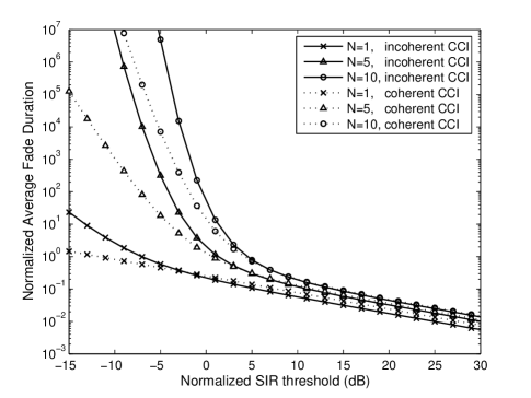
(c) Behavior of AFD

Figure 1: First-order and second-order EGC output signal statistics vs. SIR thresholds for various numbers of interferers when $M=3$

(a) Behavior of OP

(b) Behavior of average LCR

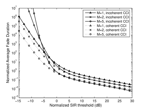
(c) Behavior of AFD

Figure 2: First-order and second-order EGC output signal statistics vs. SIR thresholds for various diversity orders when $N=5$

(a) Behavior of average LCR

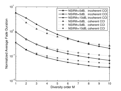
(b) Behavior of AFD

Figure 3: Second-order EGC output signal statistics vs. diversity order for various normalized SIR thresholds when $N=5$

and the normalized AFD, $f_{m0}F_{Z}/N_{Z}$ is calculated from the ratio of (39) and (40). Depending on the presumed scenario, $(\alpha,\beta)=(MN,\gamma)$ - for the incoherent interference combining, and $(\alpha,\beta)=(N,\gamma/M)$ - for the coherent interference combining, while the normalized SIR threshold (NSIRth) is determined as $\gamma/z=\Omega_{\rm S}/(\Omega_{\rm I}z)$. Note that (39) and (40) actually estimate (19b) and (34b), respectively, by sampling their integrands at equally spaced abscissas, whereas their number $L$ and locations (odd multiples of $\omega_{0}$) are given ahead of computation. There is a tradeoff between the absolute accuracy and the selection of $T$ and $L$. A larger value of $T$ results in greater accuracy, but more nonzero terms $L$ must be used [11].

(a) Behavior of average LCR

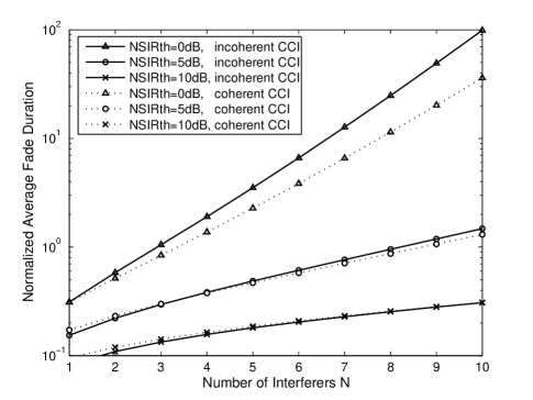
(b) Behavior of AFD

Figure 4: Second-order EGC output signal statistics vs. number of interferers for various normalized SIR thresholds when $M=2$

Using MATHEMATICA, we compared the computational burden between the two approaches/solutions by calculating the same numerical examples with same prescribed absolute accuracy of $\pm 10^{-8}$. In utilizing the first approach, we set the target accuracy into the computing software, and, for a given set of input parameters (NSIRth, $M$ and $N$), obtain the integration result and the respective value of the built-in variable that counts the number of integrand evaluations. In utilizing the second approach, the values of $T$ and $L$ needed to achieve the target accuracy are obtained empirically by trying multiple combinations of $T$ and $L$, thus yielding to typical values of $T$ between 40 and 100, and $L$ - between 100 and 200.

For a given selection of $T$ and $L$, (39) has a significantly better rate of convergence then (40), so the accuracy of (40) determines the accuracy of both the normalized AFD and normalized average LCR. Similarly, the GKQ of the OP (19b) produces a numerical result with better convergence rate and less integrand evaluations compared to the GKQ of the average LCR (34b).

We established that the first approach introduces higher computational load, thus requiring longer computation times. Namely, for the range of the input parameters shown on Figs. 1, 2 and 3, a single numeric integration using the GKQ method requires between 100 and 500 integrand evaluations to estimate a single value of the OP or the average LCR. In the same range of the input parameters, the truncated Beaulieu series typically require fewer number of integrand evaluations ($L$ nonzero terms) to achieve the same accuracy, thus yielding to shorter computation times to obtain the respective results.

It is also observed that the increase of $\alpha$ adds to the computational burden of the GKQ of both (19b) and (34b), since their integrands become more rapidly oscillatory (particularly emphasized for the average LCR calculations), thus requiring more integrand evaluations (increasing toward 500) to achieve the desired accuracy. The number of required nonzero terms $L$ in the Beaulieu series increases (toward 200) for lower NSIRth (i.e. higher threshold $z$), but rapidly decreases with the increase of the diversity order $M$. Compared to the first approach, however, the computational loads of the Beaulieu series in estimating OP and average LCR are less dependent from their input parameters.

Figs. 1 and 2 depict the OP, the normalized average LCR and the normalized AFD versus the NSIRth, with $N$ and $M$ appearing as curve parameters ($M=3$, $N=$ 1, 5 and 10 in Fig. 1, and $M=$ 1, 2 and 5, $N=$ 5 in Fig. 2). Note that if NSIRth $<$ 0 dB then $z>\Omega_{\rm S}/\Omega_{\rm I}$, while if NSIRth $>$ 0 dB then $z<\Omega_{\rm S}/\Omega_{\rm I}$.

As expected, Figs. 1a and 2a show that the OP is a monotonically decreasing function from the NSIRth, and that its values match [2, Fig. 1] and [3, Figs. 2 and 3] in the respective NSIRth ranges for given $N$ and $M$. Figs. 1b and 2b show that the average LCR reaches its maximum for some specific NSIRth, whose value depends on the selection of $M$ and $N$. Figs. 1c and 2c show that the AFD decreases by the increase of the NSIRth (i.e. by the decrease of the threshold $z$).

It is also obvious that, for a given values of NSIRth, $M$ and $N$, the average LCR and the AFD curves for incoherent and coherent interference combining almost coincide when the NSIRth is above the value that maximizes the average LCR, while they differ below this value.

Figs. 3 and 4 depict the influence of the diversity order $M$ and the number of interferers $N$ over the average LCR and the AFD for different values of NSIRth. Depending on whether NSIRth is set below or above the value that maximizes the average LCR, the average LCR may increase and/or decrease by increasing $M$ (Fig. 3a), while the AFD monotonically decreases (Fig. 3b). The average LCR may also increase and/or decrease by increasing $N$ (Fig. 4a), while the AFD monotonically increases (Fig. 4b).

Extensive Monte Carlo simulations conducted in MATLAB have validated all numeric examples presented in this Section.

V Conclusion

This paper derived the analytical expressions for the average LCR and the AFD of coherent EGC wireless communication systems subject to CCI and Rayleigh fading.

The solutions for the average LCR were derived by a novel analytical approach that circumvents the necessity of finding the explicit expression for the joint PDF of the instantaneous SIR and its time derivative. They have been expressed in forms of an infinite integral solution and an infinite series solution, assuming IID equal-powered interference signals’ replicas and IID equal-powered desired signal replicas in each diversity branch. The infinite series solutions were determined for an arbitrary diversity order after successively applying the CF method, the Parseval’s theorem and the Beaulieu series over the integral expressions for the OP and average LCR. Compared to the numerical integration method commonly implemented in the computing software packages, we concluded that the Beaulieu series solutions introduce less computational burden and minor sensitivity to the input parameters. For the dual diversity case, the average LCR and the AFD were determined as exact closed-form solutions in terms of the gamma and the beta functions.

For the interference-limited EGC systems, the desired branch signals coherently combine, while the branch signals from each interferer can combine either coherently or incoherently. Our analytical solutions incorporate both combining scenarios, yielding to somewhat different numeric values for the average LCR and the AFD. The differences are more evident when the SIR threshold is set above the average SIR per interferer per branch.

One can further alleviate the assumption for the equal branch powers of the desired signal replicas. It is straightforwardly obvious from (26) that same analytical approach is also applicable for determination of the average LCR in the case of unequal branch powers of the desired signal. The derivation of the respective solutions is trivial and omitted in this work.

Appendix A

Introducing the expressions for the CDF of $X$ (20) and the PDF of $Y$ (12) into (14), and also using [14, Eq. 3.478(1), 6.286(1)], one obtains

$$F_{G}(g)=1-\left(\frac{1}{1+g^{2}/\beta}\right)^{\alpha}-\frac{\alpha g^{2}/\beta}{[1+g^{2}/(2\beta)]^{\alpha+1}}$$

$$\times\;{}_{2}F_{1}\left(\frac{1}{2};1+\alpha;\frac{3}{2};-\frac{1}{1+2\beta/g^{2}}\right)\,,$$ (A.1)

where ${}_{2}F_{1}(a;b;c;z)$ is the Gaussian hypergeometric function [14]. We then successively apply transformations [14]

$${}_{2}F_{1}(a;b;c;z)=\left(\frac{1}{1-z}\right)^{b}\;{}_{2}F_{1}\left(c-a;b;c;\frac{z}{z-1}\right)$$ (A.2)

and

$${}_{2}F_{1}(1;b;c;z)=\frac{c-1}{z^{c-1}}(1-z)^{c-b-1}\;{\rm B}(z;c-1,b-c+1)$$ (A.3)

over (A.1) and obtain

$$F_{G}(g)=1-\left(\frac{1}{1+g^{2}/\beta}\right)^{\alpha}-\frac{\alpha\sqrt{g^{2}/(2\beta)}}{[1+g^{2}/(2\beta)]^{\alpha+1/2}}$$

$$\times\;{\rm B}\left(\frac{1/2}{1+\beta/g^{2}};\frac{1}{2},\alpha+\frac{1}{2}\right)\,.$$ (A.4)

The result (21) is obtained directly from (A.4) by setting $g=\sqrt{z}$.

Introducing the expressions for the PDF of $X$ (35) and the PDF of $Y$ (12) into (30), and also using [14, Eq. 3.478(1), 6.286(1)], one obtains

$$N_{G}(g)=\sqrt{\frac{\sigma_{\dot{X}}^{2}+g^{2}\sigma_{\dot{Y}}^{2}}{2\pi}}\;\left\{\sqrt{\frac{1}{\Omega_{\rm S}}}\frac{\Gamma(\alpha+1/2)}{\Gamma(\alpha)}\qquad\qquad\quad\right.$$

$$\times\frac{g^{2}/\sqrt{\beta}}{(1+g^{2}/\beta)^{\alpha+1/2}}+\sqrt{\frac{1}{\Omega_{\rm S}}}\frac{\Gamma(\alpha+3/2)}{\Gamma(\alpha)}\qquad\qquad\qquad$$

$$\times\;\frac{(g/\sqrt{\beta})^{3}}{(1+g^{2}/(2\beta))^{\alpha+3/2}}\;{}_{2}F_{1}\left(\frac{1}{2};\frac{3}{2}+\alpha;\frac{3}{2};-\frac{1}{1+2\beta/g^{2}}\right)$$

$$-\sqrt{\frac{1}{\Omega_{\rm S}}}\frac{\Gamma(\alpha+1/2)}{\Gamma(\alpha)}\frac{g/\sqrt{\beta}}{(1+g^{2}/(2\beta))^{\alpha+1/2}}\qquad\qquad\qquad\quad$$

$$\left.\quad\qquad\qquad\times\;{}_{2}F_{1}\left(\frac{1}{2};\frac{1}{2}+\alpha;\frac{3}{2};-\frac{1}{1+2\beta/g^{2}}\right)\right\}\,.$$ (A.5)

After successively applying both (A.2) and (A.3) over (A.5), one obtains

$$N_{G}(g)=\sqrt{\frac{\sigma_{\dot{X}}^{2}+g^{2}\sigma_{\dot{Y}}^{2}}{2\pi}}\;\left\{\sqrt{\frac{1}{\Omega_{\rm S}}}\frac{\Gamma(\alpha+1/2)}{\Gamma(\alpha)}\qquad\qquad\qquad\right.$$

$$\times\;\frac{g^{2}/\sqrt{\beta}}{(1+g^{2}/\beta)^{\alpha+1/2}}+\sqrt{\frac{1}{2\Omega_{\rm S}}}\frac{\Gamma(\alpha+3/2)}{\Gamma(\alpha)}\qquad\qquad$$

$$\times\;\frac{g^{2}/\beta}{(1+g^{2}/(2\beta))^{\alpha+1}}\;{\rm B}\left(\frac{1/2}{1+\beta/g^{2}};\frac{1}{2},1+\alpha\right)\qquad$$

$$-\sqrt{\frac{1}{2\Omega_{\rm S}}}\frac{\Gamma(\alpha+1/2)}{\Gamma(\alpha)}\frac{1}{(1+g^{2}/(2\beta))^{\alpha}}\qquad\qquad\qquad$$

$$\left.\qquad\qquad\qquad\qquad\qquad\times\;{\rm B}\left(\frac{1/2}{1+\beta/g^{2}};\frac{1}{2},\alpha\right)\right\}\,.$$ (A.6)

We further apply the following identity [14]

$${\rm B}(z;a,b+1)=\frac{z^{\alpha}(1-z)^{b}}{a+b}+\frac{b}{a+b}\;{\rm B}\left(z;a,b\right)$$ (A.7)

over (A.6), and obtain

$$N_{G}(g)=\sqrt{\frac{\sigma_{\dot{X}}^{2}+g^{2}\sigma_{\dot{Y}}^{2}}{2\pi}}\;\left\{\sqrt{\frac{1}{\Omega_{\rm S}}}\frac{\Gamma(\alpha+1/2)}{\Gamma(\alpha)}\qquad\qquad\qquad\right.$$

$$\times\frac{1}{1+g^{2}/(2\beta)}\frac{g/\sqrt{\beta}}{(1+g^{2}/\beta)^{\alpha-1/2}}+\sqrt{\frac{1}{2\Omega_{\rm S}}}\frac{\Gamma(\alpha+1/2)}{\Gamma(\alpha)}$$

$$\left.\quad\qquad\times\;\frac{(\alpha-1/2)g^{2}/\beta-1}{(1+g^{2}/(2\beta))^{\alpha+1}}\;{\rm B}\left(\frac{1/2}{1+\beta/g^{2}};\frac{1}{2},\alpha\right)\right\}\,.$$ (A.8)

The result (36) is obtained directly from (A.8) after setting $g=\sqrt{z}$.

References

- [1] G. L. Stuber, Principles of Mobile Communications, Boston: Kluwer Academic Publishers, 1996.
- [2] A. A. Abu-Dayya and N. C. Beaulieu, “Outage probabilities of diversity cellular systems with cochannel interference in Nakagami fading,” IEEE Trans. Veh. Tech., vol. VT-41, pp. 343-355, Nov. 1992.
- [3] Y. Song, S. D. Blostein and J. Cheng, “Exact Outage Probability for Equal Gain Combining With Cochannel Interference in Rayleigh Fading,” IEEE Trans. Wireless Commun., vol. 2, no. 5, pp. 865-870, Sept. 2003.
- [4] M. D. Yacoub, C. R. C. M. da Silva, and J. E. V. Bautista, “Second-order statistics for diversity-combining techniques in Nakagami-fading channels,” IEEE Trans. Veh. Technol., vol. 50, pp. 1464-1470, Nov. 2001.
- [5] C. Iskander and P. Mathiopoulos, “Analytical level crossing rates and average fade durations for diversity techniques in Nakagami fading channels,” IEEE Trans. Commun., vol. 50, no. 8, pp. 1301-1309, Aug. 2002.
- [6] N.C. Beaulieu and X. Dong, “Level Crossing Rate and Average Fade Duration of MRC and EGC Diversity in Rician Fading”, IEEE Trans. Commun., vol. 51, no. 5, pp. 722 - 726, May 2003.
- [7] L. Yang and M.-S. Alouini, “On the Average Outage Rate and Average Outage Duration of Wireless Communication Systems With Multiple Cochannel Interferers”, IEEE Trans. Wireless Commun., vol. 3, no. 4, pp. 1142 - 1153, Jul. 2004.
- [8] L. Yang and M.-S. Alouini, “Performance Comparison of Different Selection Combining Algorithms in Presence of Co-Channel Interference”, IEEE Trans. Veh. Technol., vol. 55, no. 2, pp. 559-571, Mar. 2006.
- [9] C. Tellambura and A. Annamalai, “An unified numerical approach for computing the outage probability for mobile radio systems,” IEEE Commun. Lett., vol. 3, pp. 97-99, Apr. 1999.
- [10] J. Gil-Pelaez, “Note on the inversion theorem,” Biometrika, vol. 38, pp. 481-482, 1951.
- [11] N. C. Beaulieu, “An infinite series for the computation of the complementary probability distribution function of a sum of independent random variables and its application to the sum of Rayleigh random variables,” IEEE Trans. Commun., vol. 38, pp. 1463-1474, Sept. 1990.
- [12] C. Tellambura and A. Annamalai, “Further results on the Beaulieu series,” IEEE Trans. Commun., vol. 48, pp. 1774-1777, Nov. 2000.
- [13] S. W. Halpern, “The effect of having unequal branch gains in practical predetection diversity systems for mobile radio,” IEEE Trans. Veh. Technol., vol. VT-26, pp. 94-105, Feb. 1977.
- [14] I. S. Gradshteyn and I. M. Ryzhik, Tables of Integrals, Series, and Products, 5th ed. San Diego, CA: Academic, 1994.
- [15] Y.-C. Ko, A. Abdi, M.-S. Alouini, and M. Kaveh, “Average Outage Duration of Diversity Systems over Generalized Fading Channels,” Proc. IEEE WCNC 2000, pp. 216-221, Sept. 2000.
- [16] J.-P. M. Linnartz and R. Prasad, “Threshold crossing rate and average nonfade duration in a Rayleigh-fading channel with multiple interferers,” Archiv Fur Elektron. Ubertragungstech. Electon. Commun., vol. 43, pp. 345-349, Nov./Dec. 1989.
- [17] E. W. Weisstein, “Gauss-Kronrod Quadrature,” from MathWorld - A Wolfram Web Resource, http://mathworld.wolfram.com/Gauss-KronrodQuadrature.html
- [18] D. Calvetti, G. H. Golub, W. B. Gragg, and L. Reichel, “Computation of Gauss-Kronrod Quadrature Rules,” Math. Comput., Vol. 69, No. 231, pp. 1035-1052, 2000.