Level Crossing Rate and Average Fade Duration
of Dual Selection Combining with Cochannel Interference and Nakagami Fading

Abstract

This letter provides closed-form expressions for the outage probability, the average level crossing rate (LCR) and the average fade duration (AFD) of a dual diversity selection combining (SC) system exposed to the combined influence of the cochannel interference (CCI) and the thermal noise (AWGN) in Nakagami fading channel. The branch selection is based on the desired signal power SC algorithm with all input signals assumed to be independent, while the powers of the desired signals in all diversity branches are mutually equal but distinct from the power of the interference signals. The analytical results reduce to known solutions in the cases of an interference-limited system in Rayleigh fading and an AWGN-limited system in Nakagami fading. The average LCR is determined by an original approach that does not require explicit knowledge of the joint PDF of the envelope and its time derivative, which also paves the way for similar analysis of other diversity systems.

I Introduction

Diversity is often used to mitigate fading in wireless communication systems and selection combining (SC) is one of the simplest diversity combining methods [1]. The outage probability (OP) is the first-order statistical measure of a diversity system and its typical performance measure. The OP of SC systems in an interference-limited environment (such as that of cellular mobile systems) for various fading channels presented a challenge that was successfully tackled by the studies of more then a few researchers, for example, for the Rayleigh channel in [2], for the Nakagami channel in [3]-[5], and for the correlated Nakagami channels in [6]. The OP is also essential to determine other system’s performance measures, such as the probabilities of bit (symbol) error that are also already determined for various modulation techniques and corresponding SC receiver structures and fading channels [5], [6]. The average level crossing rate (LCR) and the average fade duration (AFD) are the system second-order statistical measures [7]-[9], which reflect the correlation properties of its input/output signals. The expressions for the average LCR and the AFD are known for the signal envelope at the output of an SC system for independent branch (Rayleigh, Rician or Nakagami fading) signals in presence of the thermal noise (AWGN) but in absence of the cochannel interference (CCI) [10]. In [11], explicit closed-form expressions are derived for the average LCR and the AFD of a dual diversity SC system subject to CCI and Rayleigh fading only. In this letter, we derive the expressions for the average LCR and the AFD for the dual diversity SC system that employs the desired signal power algorithm and is exposed to both the AWGN and the CCI in generalized Nakagami fading channels.

II System and Channel Models

The dual diversity SC communication receiver is exposed to the AWGN and independent and identically distributed (IID) single desired signal and multiple CCI signals transmitted over Nakagami flat fading channels. The desired signal is received over two diversity branches (paths) with same set of average fading power $\Omega_{\rm S}$ and fading severity parameter $m_{\rm S}$, whose envelopes $x_{0k}\>(1\leq k\leq 2)$ follow the Nakagami probability distribution function (PDF) [12],

$$f_{x_{0k}}(x)=\left(\frac{m_{\rm S}}{\Omega_{\rm S}}\right)^{m_{\rm S}}\frac{2x^{2m_{\rm S}-1}}{\Gamma(m_{\rm S})}\exp\left(-\frac{m_{\rm S}x^{2}}{\Omega_{\rm S}}\right),\,x\geq 0,$$ (1)

where $\Gamma(\cdot)$ is the Gamma function, defined by $\Gamma(a)=\int_{0}^{\infty}t^{a-1}e^{-t}dt$ [14].

The cochannel interference consists of $n$ Nakagami-faded IID transmissions (each received over the two diversity branches). They are assumed to have same set of average fading power $\Omega_{\rm I}$ and fading severity parameter $m_{\rm I}$, so the envelope of some interference signal $i\,(1\leq i\leq n)$ received in branch $k$, $w_{ik}$, is a Nakagami random variable (RV) whose PDF is given by [12]

$$f_{w_{ik}}(w)=\left(\frac{m_{\rm I}}{\Omega_{\rm I}}\right)^{m_{\rm I}}\frac{2w^{2m_{\rm I}-1}}{\Gamma(m_{\rm I})}\exp\left(-\frac{m_{\rm I}w^{2}}{\Omega_{\rm I}}\right),w\geq 0.$$ (2)

Both $m_{\rm S}$ and $m_{\rm I}$ are assumed to be positive integers.

In presence of the CCI, the branch selection of the selective combiners can rely on three somewhat different decision algorithms that already received sufficient attention in the literature [3, Section IV] and [11]: the desired signal power algorithm, the total power algorithm and the signal-to-interference power ratio (SIR) algorithm. The desired signal power algorithm is the most difficult to implement in practice as it requires identification and separation of the desired signal and the CCI. However, the known performance analysis of the desired signal power algorithm for an interference-limited SC system (the outage probability [3] and the LCR and AFD in Rayleigh fading [11]) indicates almost identical performance to that of the total power algorithm, which is the easiest to implement in practice. For the purpose of analytical tractability, we adopt the desired signal power algorithm and reasonably assume that the obtained results may also closely indicate the performance of the total power algorithm.

Note that the presence of the AWGN does not significantly influence the operation of the desired signal power algorithm and its decisions. This assumption is appropriate only if, in measuring the largest desired signal power, the average AWGN power is taken over a sufficiently long time such that it may be considered as a constant across all branches. In this case, choosing the signal with the largest desired signal power is actually equivalent to choosing the branch with the largest signal-to-noise power ratio (SNR).

Thus, the receiver is assumed to use the SC algorithm that selects the branch with the largest short-term desired signal power, $x^{2}_{0}=\max\{x^{2}_{01},x^{2}_{02}\}$, or, equivalently, the desired branch signal with the largest short-term envelope level, $x_{0}=\max\{x_{01},x_{02}\}$. Then, the short-term interference power at the output of the SC receiver is consisted of the powers of the individual interference signals $w_{i}$ received in the selected branch, and is given by $w^{2}=\sum_{i=1}^{n}w^{2}_{i}$ [3, Eqs. (19)-(22)] where the PDF of $w_{i}$ is determined by (2). Considering also the presence of the AWGN, the short-term signal-to-interference-plus-noise power ratio (SINR) at the output of the dual diversity SC system is given by [6]

$$z=\frac{\max\left(\{x^{2}_{0k}\}_{k=1}^{2}\right)}{\sum_{i=1}^{n}w^{2}_{i}+\sigma^{2}}=\frac{x^{2}_{0}}{y^{2}}\,,$$ (3)

where $\sigma^{2}$ is the AWGN power (being constant over the short-term measurement and equal for the two diversity branches) and $y^{2}=w^{2}+\sigma^{2}$ is the interference-plus-noise power. For an interference-limited system, $\sigma^{2}=0$, and (3) reduces to $z_{\rm I}=x^{2}_{0}/w^{2}$, denoting the short-term SIR.

III Average LCR and AFD

III-A Definitions

To arrive at the desired result, we define the ratio of the selected desired signal envelope $x_{0}$ and the interference-plus-noise envelope $y$,

$$g=\sqrt{z}\,\stackrel{{\scriptstyle\rm def}}{{=}}\frac{x_{0}}{y}\,,$$ (4)

which will be denoted as the envelope ratio. In absence of the AWGN, the envelope ratio is represented as $g_{\rm I}=\sqrt{z_{\rm I}}\stackrel{{\scriptstyle\rm def}}{{=}}x_{0}/w$, denoting the signal-to-interference envelope ratio.

We will first establish the average LCR of the envelope ratio. The average LCR of the envelope ratio at threshold $g$ represents the average number of times, per time unit, the stationary fading process $g(t)$ crosses threshold $g$ in the positive direction, and is mathematically defined by Rice’s formula [7]

$$N_{g}(g)=\int_{0}^{\infty}{\dot{g}}f_{g\dot{g}}(g,\,\dot{g})d\dot{g},$$ (5)

where $\dot{g}$ denotes the time derivative of $g$, and $f_{g\dot{g}}(g,\dot{g})$ is the joint PDF of RVs $g$($t$) and $\dot{g}(t)$ in an arbitrary moment $t$. The AFD is defined as the average time that the envelope ratio remains below the threshold $g$, and is defined by

$$T_{g}(g)=\frac{F_{g}(g)}{N_{g}(g)}\,,$$ (6)

where $F_{g}(\cdot)$ denotes the cumulative distribution function (CDF) of the envelope ratio. By introducing (4) into (5) and (6), the average LCR and the AFD for the SINR at threshold $z$ are found as $N_{z}(z)=N_{g}(\sqrt{z})$ and $T_{z}(z)=T_{g}(\sqrt{z})$, respectively.

III-B Outage Probability

First, let us determine the PDF of the envelope ratio at the SC receiver output. It is calculated from [13, Eq. (2)] applied over (4),

$$f_{g}(g)=\int_{0}^{\infty}yf_{x_{0}}(gy)f_{y}(y)dy\,,$$ (7)

where $f_{x_{0}}(\cdot)$ is the PDF of the selected desired signal envelope $x_{0}$. It is well known that this PDF can be represented in terms of the envelope PDFs and the envelope CDFs of the two desired signals as $f_{x_{0}}(x)=F_{x_{01}}(x)f_{x_{02}}(x)+F_{x_{02}}(x)f_{x_{01}}(x)$. In Nakagami fading, $f_{x_{01}}(x)=f_{x_{02}}(x)$ are determined by (1), while the respective CDFs by $F_{x_{01}}(x)=F_{x_{02}}(x)=1-\Gamma(m_{\rm S},m_{\rm S}x^{2}/\Omega_{\rm S})/\Gamma(m_{\rm S})$, where $\Gamma(\cdot,\cdot)$ is the incomplete Gamma function defined by $\Gamma(a,z)=\int_{z}^{\infty}t^{a-1}e^{-t}dt$ [14]. Thus, the PDF of $x_{0}$ is determined as

$$f_{x_{0}}(x)=\left(\frac{m_{\rm S}}{\Omega_{\rm S}}\right)^{m_{\rm S}}\frac{4x^{2m_{\rm S}-1}}{\Gamma(m_{\rm S})}\exp\left(-\frac{m_{\rm S}x^{2}}{\Omega_{\rm S}}\right)$$

$$\times\left(1-\frac{1}{\Gamma(m_{\rm S})}\Gamma\left(m_{\rm S},\frac{m_{\rm S}x^{2}}{\Omega_{\rm S}}\right)\right), x\geq 0.$$ (8)

When $m_{\rm S}$ is a positive integer, $\Gamma(\cdot,\cdot)$ is represented as the finite series expansion given by (A.1) in Appendix A. The envelope PDF of the output interference signal $w$ is given by

$$f_{w}(w)=\left(\frac{m_{\rm I}}{\Omega_{\rm I}}\right)^{m_{\rm I}n}\frac{2w^{2m_{\rm I}n-1}}{\Gamma(m_{\rm I}n)}\,\exp\left(-\frac{m_{\rm I}w^{2}}{\Omega_{\rm I}}\right),\,w\geq 0,$$ (9)

while, by using the standard transformation theory over the RV $y=\sqrt{w^{2}+\sigma^{2}}$, the PDF of the output interference-plus-noise envelope $y$ is obtained as

$$f_{y}(y)=\left(\frac{m_{\rm I}}{\Omega_{\rm I}}\right)^{m_{\rm I}n}\,\frac{2y(y^{2}-\sigma^{2})^{m_{\rm I}n-1}}{\Gamma(m_{\rm I}n)}\qquad\;$$

$$\times\exp\left(-\frac{m_{\rm I}}{\Omega_{\rm I}}\left(y^{2}-\sigma^{2}\right)\right), y\geq\sigma.$$ (10)

Applying (8) and (10) over (7), it is possible to obtain the closed-form solution for the PDF of the envelope ratio as according to the derivation given in Appendix A, which is

$$f_{g}(g)=\frac{4}{\sqrt{\mu}}\frac{(g^{2}/\mu)^{m_{\rm S}-1/2}\,\,\exp(\sigma^{2}m_{\rm I}/\Omega_{\rm I})}{\Gamma(m_{\rm S})\Gamma(m_{\rm I}n)}\qquad\qquad\;\;$$

$$\times\sum_{i=1}^{m_{\rm I}n}{{m_{\rm I}n-1}\choose{i-1}}\left(-\frac{\sigma^{2}m_{\rm I}}{\Omega_{\rm I}}\right)^{m_{\rm I}n-i}\left[\frac{1}{(1+g^{2}/\mu)^{m_{\rm S}+i}}\right.$$

$$\left.\times\,\Gamma\left(m_{\rm S}+i,\frac{m_{\rm I}\sigma^{2}}{\Omega_{\rm I}}(1+\frac{g^{2}}{\mu})\right)\right.\qquad\qquad\quad$$

$$-\frac{1}{(1+2g^{2}/\mu)^{m_{\rm S}+i}}\sum_{j=0}^{m_{\rm S}-1}\frac{1}{j!}\left(\frac{g^{2}/\mu}{1+2g^{2}/\mu}\right)^{j}$$

$$\qquad\times\,\Gamma\left.\left(m_{\rm S}+i+j,\,\frac{m_{\rm I}\sigma^{2}}{\Omega_{\rm I}}(1+2\frac{g^{2}}{\mu})\right)\right],$$ (11)

where $\mu$ represents the ratio of the average scattered powers of the selected desired signal and a single interference signal, given by $\mu=(\Omega_{\rm S}m_{\rm I})/(\Omega_{\rm I}m_{\rm S})$.

The PDF of the SINR is obtained directly from (11) according $f_{z}(z)=f_{g}(\sqrt{z})/(2\sqrt{z})$. The CDF of the SINR at threshold $z$ is obtained by introducing (11) into $F_{z}(z)=\int_{0}^{\sqrt{z}}f_{g}(g)dg$, which actually represents the OP of the SC system.

It is possible to determine the closed-form solution of the CDF of the SINR, because the first arguments of the incomplete Gamma function appearing in (11) are positive integers and are expandable as finite series according to (A.1). This expansion will yield to simpler definite integrals solvable in closed-form involving additional finite series, as follows

$$\int_{0}^{z/\mu}t^{a-1}(1+t)^{-b}e^{-ct}dt=(-1)^{a}e^{c}c^{b-1}\sum_{k=0}^{a-1}{{a-1}\choose k}$$

$$(-c)^{-k}[\Gamma(k+1-b,c(1+z/\mu))-\Gamma(k+1-b,c)]\,,$$ (12)

where $a$ and $b$ are positive integers, and $c=\sigma^{2}m_{\rm I}/\Omega_{\rm I}$. As a result, the closed-form solution of the CDF of the SINR involves five-fold summations and will not be presented here due to its length. Alternatively, it is possible to numerically integrate (11) by using standard numerical techniques and to determine the CDF of the SINR for the given set of values for $z$, $\mu$ and $c$.

For an interference-limited system, (11) specializes into a closed-form representing the PDF of the signal-to-interference envelope ratio,

$$f_{g_{\rm I}}(g)=\frac{4}{\sqrt{\mu}}\frac{1}{{\rm B}(m_{\rm S},m_{\rm I}n)}\frac{(g^{2}/\mu)^{m_{\rm S}-1/2}}{(1+g^{2}/\mu)^{m_{\rm S}+m_{\rm I}n}}\qquad$$

$$\times\,{I}\left(\frac{1}{2+\mu/g^{2}};m_{\rm S},m_{\rm S}+m_{\rm I}n\right),$$ (13)

which is also derived in Appendix A. In (13), ${\rm B}(\cdot,\cdot)$ is the Beta function ${\rm B}(a,b)=\Gamma(a)\Gamma(b)/\Gamma(a+b)$, and ${I}(\cdot;\cdot,\cdot)$ is the regularized Beta function defined by ${I}(z;a,b)\equiv{I}_{z}(a,b)={\rm B}_{z}(a,b)/{\rm B}(a,b)$, where ${\rm B}_{z}(\cdot,\cdot)$ is the incomplete Beta function defined by ${\rm B}_{z}(a,b)\equiv{\rm B}(z;a,b)=\int_{0}^{z}t^{a-1}(1-t)^{b-1}dt$ [14].

When $m_{\rm S}$ is a positive integer, a closed-form solution for the respective CDF is obtainable in terms of the Beta functions as given in Appendix A by (A). Consequently, the CDF of the SIR at threshold $z$ is given by

$$F_{z_{\rm I}}(z)=\frac{2(-1)^{m_{\rm S}}}{{\rm B}(m_{\rm S},m_{\rm I}n)}\,{\rm B}\left(-\frac{z}{\mu};m_{\rm S},1-m_{\rm S}-m_{\rm I}n\right)$$

$$+\,\frac{1}{{\rm B}(m_{\rm S},m_{\rm I}n)}\left(-\frac{1}{2}\right)^{m_{\rm S}-1}\,\sum_{j=0}^{m_{\rm S}-1}{{m_{\rm S}+m_{\rm I}n+j-1}\choose j}$$

$$\times\left(-\frac{1}{2}\right)^{j}{\rm B}\left(-\frac{2z}{\mu};m_{\rm S}+j,1-m_{\rm S}-m_{\rm I}n-j\right),$$ (14)

In case of Rayleigh fading ($m_{\rm S}=m_{\rm I}=1$), using the general identity ${\rm B}(z;1,b)=(1-(1-z)^{b})/b$, it is readily verified that (14) specializes into a previously obtained result [11, Eq. (33)].

The results (11), (13) and (14) are new to the best of the author’s knowledge.

III-C General Expression for Average LCR

As according to (4), the random process $g(t)$ is related to the envelopes of the desired signals $x_{0k}(t)$ and the interference signals received in the selected branch $w_{i}(t)$. For an arbitrary power spectrum and certain mathematical conditions, each envelope’s time derivative at any given moment $t$ follows the zero-mean Gaussian PDF [7]-[9] and is statistically independent from its envelope [8], [9]. Assuming a continuous wave (CW) transmission and two-dimensional isotropic scattering, the Clarke’s model determines the variance of this Gaussian PDF to be given by $\sigma_{\dot{x}_{0k}}^{2}=(\pi f_{m0})^{2}\Omega_{\rm S}/m_{\rm S}$ and $\sigma_{\dot{w}_{i}}^{2}=(\pi f_{mi})^{2}\Omega_{\rm I}/m_{\rm I}$ for each of the desired signal and the interference signals, respectively [9]. It is also assumed that the maximum Doppler spreads of the two desired signals $x_{0k}$ are equal to $f_{m0}$, and the maximum Doppler spreads of all interference signals $w_{i}$ are equal to $f_{mi}$.

To determine the average LCR of the random process $g(t)$ by using definition (5), one needs to establish the joint PDF of random processes $g(t)$ and $\dot{g}(t)$ at any given moment $t$. However, we utilize an alternative approach, which circumvents explicit determination of $f_{g\dot{g}}(g,\dot{g})$. From (4), the time derivative of the envelope ratio is written as

$$\dot{g}=\frac{1}{y}\,\dot{x}_{0}-\frac{x_{0}}{y^{2}}\,\dot{y}=\frac{1}{y}\,\dot{x}_{0}-\frac{g}{y}\,\dot{y}\,.$$ (15)

Conditioned on $y$, the joint PDF $f_{g\dot{g}}(g,\dot{g})$ is calculated as

$$f_{g\dot{g}}(g,\dot{g})=\int_{0}^{\infty}f_{g\dot{g}|y}(g,\dot{g}|y)\,f_{y}(y)dy\,,$$ (16)

where $f_{y}(y)$ is the PDF of the interference-plus-noise envelope $y$ given by (10).

In (16), $f_{g\dot{g}|y}(g,\dot{g}|y)$ is the conditional joint PDF of $g$ and $\dot{g}$ given some specified value of the interference-plus-noise envelope $y$, which is expressed as

$$f_{g\dot{g}|y}(g,\dot{g}|y)=f_{\dot{g}|gy}(\dot{g}|g,y)\,f_{g|y}(g|y)\,,$$ (17)

where $f_{g|y}(g|y)$ is the conditional PDF of $g$ given some specified value of $y$. From (4), $f_{g|y}(g|y)=yf_{x_{0}}(gy)$, where $f_{x_{0}}(\cdot)$ is the PDF of the selected desired signal envelope $x_{0}$.

In (17), $f_{\dot{g}|gy}(\dot{g}|g,y)$ is the conditional PDF of $\dot{g}$ given some specified values of the envelopes ratio $g$ and interference-plus-noise envelope $y$. Considering (15), this conditional PDF is determined as follows: Conditioned on $g$ and $y$, $\dot{g}$ is a linear combination of two independent RVs: the time derivative of the selected desired signal envelope $\dot{x}_{0}(t)$ and the time derivative of the interference-plus-noise envelope $\dot{y}(t)$.

We now represent the output interference-plus-noise power as a constant plus a sum of $m_{\rm I}n$ IID squared Rayleigh RVs $\alpha_{ij}$ as $y^{2}=\sigma^{2}+\sum_{i=1}^{n}\sum_{j=1}^{m_{\rm I}}\alpha^{2}_{ij}$, since $m_{\rm I}$ is a positive integer. After deriving both sides of the latter expression with respect to $t$, constant $\sigma^{2}$ vanishes so that we can apply the result [15, Section 3.2.1] and conclude that the time derivative of the interference-plus-noise envelope $\dot{y}(t)$ is a zero-mean Gaussian RV with variance equal to the variance of $\dot{w}_{i}(t)$ of any interferer ($\sigma^{2}_{\dot{y}}=\sigma^{2}_{\dot{w}_{i}}$), but only if $\sigma^{2}_{\dot{w}_{i}}$ is equal for all $i$, as assumed in our case.

Based on [10, Eqs. (13)-(15)], we also conclude that the SC output signal envelope $x_{0}(t)$ and its time derivative $\dot{x}_{0}(t)$ are independent RVs at any given $t$, and that $\dot{x}_{0}(t)$ is a zero-mean Gaussian RV with variance equal to the variance of $\dot{x}_{0k}(t)$ of any desired signal ($\sigma^{2}_{\dot{x}_{0}}=\sigma^{2}_{\dot{x}_{0k}}$), since $\sigma^{2}_{\dot{x}_{0k}}$ is assumed equal for both $k$ (and $x_{0k}$s are IID RVs at any given $t$). Consequently, $\dot{g}$ is a zero-mean Gaussian RV with variance

$$\sigma^{2}_{\dot{g}|gy}=\frac{1}{y^{2}}\,\sigma^{2}_{\dot{x}_{0}}+\frac{g^{2}}{y^{2}}\,\sigma^{2}_{\dot{y}}\,\,.$$ (18)

Introducing (16) and (17) into (5), and changing the orders of integration, we obtain

$$N_{g}(g)=\int_{0}^{\infty}\dot{g}d\dot{g}\int_{0}^{\infty}f_{\dot{g}|gy}(\dot{g}|g,y)\,f_{g|y}(g|y)\,f_{y}(y)dy$$

$$=\int_{0}^{\infty}f_{g|y}(g|y)\,f_{y}(y)dy\int_{0}^{\infty}\dot{g}\,f_{\dot{g}|gy}(\dot{g}|g,y)d\dot{g}\,\,.$$ (19)

The inner integral in (19) is calculated by using (18), i.e.,

$$\int_{0}^{\infty}\dot{g}\,f_{\dot{g}|gy}(\dot{g}|g,y)\,d\dot{g}=\frac{\sigma_{\dot{g}|gy}}{\sqrt{2\pi}}=\frac{1}{y}\,\sqrt{\frac{\sigma^{2}_{\dot{x}_{0}}+g^{2}\sigma^{2}_{\dot{w}_{i}}}{2\pi}}\,.$$ (20)

Substituting (20) into (19) and considering that $f_{g|y}(g|y)=yf_{x_{0}}(gy)$, we arrive at the important generalized expression for the average LCR of the envelope ratio at threshold $g$,

$$N_{g}(g)=\sqrt{\frac{\sigma^{2}_{\dot{x}_{0}}+g^{2}\sigma^{2}_{\dot{w}_{i}}}{2\pi}}\,\int_{0}^{\infty}f_{x_{0}}(gy)\,f_{y}(y)dy\,.$$ (21)

In absence of CCI, $\Omega_{\rm I}=0$ and the PDF of $y$ is given by $f_{y}(y)=\delta(y-\sigma)$, where $\delta(\cdot)$ is the Dirac delta function. In this case, the envelope ratio actually represents the signal-to-noise envelope ratio $g_{\rm N}=x_{0}/\sigma$, whose average LCR is obtained from (21) after applying the fundamental property of the Dirac delta function,

$$N_{g_{\rm N}}(g)=\frac{\sigma_{\dot{x}_{0}}}{\sqrt{2\pi}}f_{x_{0}}(\sigma g)\,.$$ (22)

Introduction of (8) into (22) yields to an expression consistent with [10, Eq. (18c)] for the case of dual diversity SC.

III-D Average LCR for Our System and Channel Models

Applying (8) and (10) over (21), it is possible to obtain the closed-form solution for the average LCR of the envelope ratio at threshold $g$ as according to the derivation given in Appendix B, and then determine the average LCR of the SINR at threshold $z$ as follows

$$N_{z}(z)=\sqrt{8\pi}\sqrt{f^{2}_{m0}+f^{2}_{mi}z/\mu}\frac{(z/\mu)^{m_{\rm S}-1/2}\exp(\sigma^{2}m_{\rm I}/\Omega_{\rm I})}{\Gamma(m_{\rm S})\Gamma(m_{\rm I}n)}$$

$$\times\sum_{i=1}^{m_{\rm I}n}{{m_{\rm I}n-1}\choose{i-1}}\left(-\frac{\sigma^{2}m_{\rm I}}{\Omega_{\rm I}}\right)^{m_{\rm I}n-i}\left[\frac{1}{(1+z/\mu)^{m_{\rm S}+i-1/2}}\right.$$

$$\left.\times\,\Gamma\left(m_{\rm S}+i-\frac{1}{2},\frac{\sigma^{2}m_{\rm I}}{\Omega_{\rm I}}\left(1+\frac{z}{\mu}\right)\right)\right.\qquad\qquad\quad\;\;$$

$$-\frac{1}{(1+2z/\mu)^{m_{\rm S}+i-1/2}}\sum_{j=0}^{m_{\rm S}-1}\frac{1}{j!}\left(\frac{z/\mu}{1+2z/\mu}\right)^{j}\qquad$$

$$\quad\quad\left.\times\,\Gamma\left(m_{\rm S}+i+j-\frac{1}{2},\frac{\sigma^{2}m_{\rm I}}{\Omega_{\rm I}}\left(1+\frac{2z}{\mu}\right)\right)\right].$$ (23)

For an interference-limited system, (23) specializes into a closed-form that represents the average LCR of the SIR at threshold $z$,

$$N_{z_{\rm I}}(z)=\sqrt{8\pi}\,\sqrt{f^{2}_{m0}+f^{2}_{mi}z/\mu}\,\frac{\Gamma(m_{\rm S}+m_{\rm I}n-1/2)}{\Gamma(m_{\rm S})\Gamma(m_{\rm I}n)}$$

$$\times\frac{(z/\mu)^{m_{\rm S}-1/2}}{(1+z/\mu)^{m_{\rm S}+m_{\rm I}n-1/2}}\,{I}\left(\frac{1}{2+\mu/z};m_{\rm S},m_{\rm S}+m_{\rm I}n-\frac{1}{2}\right).$$ (24)

The derivation of the respective LCR of the signal-to-interference envelope ratio is provided in Appendix B. For the two-dimensional isotropic scattering and CW transmissions with same maximum Doppler spreads ($f_{mi}=f_{m0}$), $\sigma^{2}_{\dot{x}_{0}}/\sigma^{2}_{\dot{w}_{i}}=\mu$ and (24) further reduces into

$$N_{z_{\rm I}}(z)=\sqrt{8\pi}f_{m0}\frac{\Gamma(m_{\rm S}+m_{\rm I}n-1/2)}{\Gamma(m_{\rm S})\Gamma(m_{\rm I}n)}\frac{(z/\mu)^{m_{\rm S}-1/2}}{(1+z/\mu)^{m_{\rm S}+m_{\rm I}n-1}}$$

$$\qquad\qquad\qquad\times\,{I}\left(\frac{1}{2+\mu/z};m_{\rm S},m_{\rm S}+m_{\rm I}n-\frac{1}{2}\right).$$ (25)

In case of Rayleigh fading ($m_{\rm S}=m_{\rm I}=1$), using the general identity ${I}(z;1,b)=1-(1-z)^{b}$, it is readily verified that (25) specializes into the known result [11, Eq. (32)]. The results (23), (24) and (25) are new to the best of the author’s knowledge.

Without any loss in generality of the obtained expressions for both the OP and the average LCR, it is possible to set $\sigma^{2}=1$ while replacing the average desired signal power $\Omega_{\rm S}$ with the average SNR per interferer per branch $\gamma_{\rm S}=\Omega_{\rm S}/\sigma^{2}$ and the average interference power $\Omega_{\rm I}$ - with the average interference-to-noise power ratio (INR) per interferer per branch $\gamma_{\rm I}=\Omega_{\rm I}/\sigma^{2}$. In this case, $\Omega_{\rm S}/\Omega_{\rm I}=\gamma_{\rm S}/\gamma_{\rm I}$ and $\mu=(\gamma_{\rm S}m_{\rm I})/(\gamma_{\rm I}m_{\rm S})$.

The AFD of the SINR at the output of the SC receiver at threshold $z$ is obtained from $T_{z}(z)=F_{z}(z)/N_{z}(z)$.

(a) Behavior of average LCR

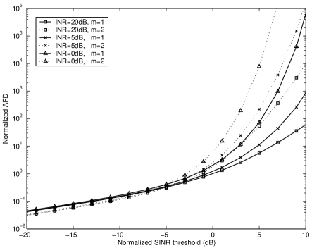
(b) Behavior of AFD

Figure 1: Second-order output signal statistics of dual diversity SC system with CCI and AWGN vs. SINR threshold for various INRs ($\gamma_{\rm I}$) and fading parameters ($m=m_{\rm S}=m_{\rm I}$) when $n=3$

IV Numeric Results

Figs. 1 and 2 illustrate the behavior of the second-order statistical measures at the output of a dual diversity SC system, assuming all CW transmitted signals were exposed to two-dimensional isotropic scattering, same maximum Doppler spreads ($f_{mi}=f_{m0}$) and same fading severity ($m_{\rm S}=m_{\rm I}$).

Fig. 1 shows the plots of the normalized LCR $N_{z}(z)/f_{m0}$ and the normalized AFD $T_{z}(z)f_{m0}$ in function of the normalized SINR threshold $z/\mu$ (NSINRth) for different values of $m_{\rm S}$ and $\gamma_{\rm I}$ when $n=3$. For given $m_{\rm S}$ and $\gamma_{\rm I}$, the average LCR increases with the increase of NSINRth until it reaches its maximum at NSINRth$=th_{0}$, and then decreases (Fig. 1a). Note that $th_{0}$ depends on $\gamma_{\rm I}$ and $m_{\rm S}$, since $n$ is fixed. As expected, the AFD is a monotonically increasing function of NSINRth, which is depicted in Fig. 1b.

The average LCR is decreased when the system is exposed to a less severe fading channel (i.e. signal envelopes fluctuate less rapidly around their means), which is illustrated in Fig. 1a by the increase of $m_{\rm S}$ from 1 to 2. Increasing $m_{\rm S}$, the AFD is only slightly decreased for NSINRth below $th_{0}$, and is significantly increased for NSINRth above $th_{0}$ as the output SINR spends more time around its mean (Fig. 1b).

When NSINRth is fixed to a value below its respective $th_{0}$, the increase of $\gamma_{\rm I}$ from 0 to 20 dB results in only a minor decrease of the average LCR, while the AFD is almost unaltered. For values of NSINRth above $th_{0}$, increasing $\gamma_{\rm I}$ results in the significant increase of the average LCR (Fig. 1a) and the decrease of the AFD (Fig. 1b).

When the SC system is interference-limited, Fig. 2 displays $N_{Z_{\rm I}}(z)/f_{m0}$ and $T_{Z_{\rm I}}(z)f_{m0}$ versus the number of interfering users $n$ for different values of the normalized SIR threshold $z/\mu$ (NSIRth) when $m_{\rm S}=2$. The average LCR can increase and/or decrease by varying $n$, which depends on whether NSIRth is selected below or above its $th_{0}$ (note that $th_{0}$ now depends only from $n$). The AFD is a monotonically increasing function of $n$ regardless of the selection of NSIRth (Fig. 2b).

(a) Behavior of average LCR

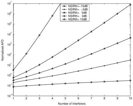
(b) Behavior of AFD

Figure 2: Second-order output signal statistics of dual diversity SC system with CCI vs. number of interfering users for various SIR thresholds when $m_{\rm S}=m_{\rm I}=2$

V Concluding Remarks

In this letter, we provide the analysis of the second-order statistical signal properties at the output of the SC systems exposed to the combined influence of the CCI and the AWGN, which was not previously available in the literature.

The expression (21) is particularly important since it provides solution for the average LCR of the SINR for the SC system that uses the desired signal power algorithm in arbitrary fading conditions, under the assumption of equal-powered IID interference signals in all diversity branches. It incorporates the solutions for the average LCRs in the special cases - when the SC system is exposed only to the influence of the AWGN or only to the influence of the CCI. If the closed-form solution of (21) is not obtainable for some specific fading scenario, it is possible to apply some known numeric integration technique and obtain the desired numeric result with predefined accuracy for a given set of input parameters. Furthermore, it can readily be proved that (21) is also valid for other diversity techniques, such as the maximal ratio combing (MRC) and the equal gain combining (EGC).

Appendix A

The finite series expansion of the incomplete Gamma function $\Gamma(\cdot,\cdot)$, valid for positive integer values of $m_{\rm S}$, is given by [14]

$$\Gamma\Big{(}m_{\rm S},\frac{m_{\rm S}x^{2}}{\Omega_{\rm S}}\Big{)}=\Gamma(m_{\rm S})\exp\left(-\frac{m_{\rm S}x^{2}}{\Omega_{\rm S}}\right)\sum_{j=0}^{m_{\rm S}-1}\frac{1}{j!}\left(\frac{m_{\rm S}x^{2}}{\Omega_{\rm S}}\right)^{j}$$ (A.1)

The finite series expansion of (10) is obtained by using the binomial formula, so

$$f_{y}(y)=\sum_{i=0}^{m_{\rm I}n-1}{{m_{\rm I}n-1}\choose i}\left(\frac{m_{\rm I}}{\Omega_{\rm I}}\right)^{m_{\rm I}n}(-\sigma^{2})^{{m_{\rm I}n-i-1}}$$

$$\times\exp\left(\frac{m_{\rm I}\sigma^{2}}{\Omega_{\rm I}}\right)\frac{2y^{2i+1}}{\Gamma(m_{\rm I}n)}\exp\left(-\frac{m_{\rm I}y^{2}}{\Omega_{\rm I}}\right),\,y\geq\sigma.$$ (A.2)

We now introduce (8), (A.1) and (A) into (7), change the order of summation and integration, solve the inner integrals in terms of the incomplete Gamma function $\Gamma(\cdot,\cdot)$, perform some algebraic manipulations, and obtain

$$f_{g}(g)=\sum_{i=0}^{m_{\rm I}n-1}{{m_{\rm I}n-1}\choose i}(-\sigma^{2})^{m_{\rm I}n-1-i}\,\,e^{(m_{\rm I}\sigma^{2}/\Omega_{\rm I})}\,\Phi_{i}(g)$$ (A.3)

where

$$\Phi_{i}(g)=\int_{\sigma}^{\infty}\left(\frac{m_{\rm I}}{\Omega_{\rm I}}\right)^{m_{\rm I}n}\frac{2y^{2i+2}}{\Gamma(m_{\rm I}n)}\exp\left(-\frac{m_{\rm I}y^{2}}{\Omega_{\rm I}}\right)f_{x_{0}}(gy)dy$$

$$=\frac{4}{\sqrt{\mu}}\frac{(g^{2}/\mu)^{m_{\rm S}-1/2}}{\Gamma(m_{\rm S})\Gamma(m_{\rm I}n)}\left(\frac{m_{\rm I}}{\Omega_{\rm I}}\right)^{m_{\rm I}n-i-1}\left[\frac{1}{(1+g^{2}/\mu)^{m_{\rm S}+i+1}}\right.$$

$$\times\,\Gamma\left(m_{\rm S}+i+1,\frac{\sigma^{2}m_{\rm I}}{\Omega_{\rm I}}(1+g^{2}/\mu)\right)\qquad\qquad$$

$$-\frac{1}{(1+2g^{2}/\mu)^{m_{\rm S}+i+1}}\left.\sum_{j=0}^{m_{\rm S}-1}\frac{1}{j!}\left(\frac{g^{2}/\mu}{1+2g^{2}/\mu}\right)^{j}\right.$$

$$\qquad\qquad\;\;\left.\times\,\Gamma\left(m_{\rm S}+i+j+1,\frac{\sigma^{2}m_{\rm I}}{\Omega_{\rm I}}(1+2g^{2}/\mu)\right)\right].$$ (A.4)

Expression (11) is obtained directly from (A.3) and (A) by introducing the substitution for summation index $i\rightarrow i+1$.

When the SC system is interference-limited, we apply the limes over (A.3) and (A) when $\sigma^{2}\rightarrow 0$. In this case, only the last term of the sum in (A.3), $i=m_{\rm I}n-1$, remains non-zero, while the incomplete Gamma functions in (A) are transformed into the respective Gamma functions, so the PDF of the signal-to-interference envelope ratio becomes

$$f_{g_{\rm I}}(g)=\frac{4}{\sqrt{\mu}}\frac{(g^{2}/\mu)^{m_{\rm S}-1/2}}{\Gamma(m_{\rm S})\Gamma(m_{\rm I}n)}\Big{[}\frac{\Gamma(m_{\rm S}+m_{\rm I}n)}{(1+g^{2}/\mu)^{m_{\rm S}+m_{\rm I}n}}\qquad$$

$$-\frac{1}{(1+\frac{2g^{2}}{\mu})^{m_{\rm S}+m_{\rm I}n}}\sum_{j=0}^{m_{\rm S}-1}\frac{\Gamma({m_{\rm S}+m_{\rm I}n}+j)}{j!}\Big{(}\frac{g^{2}/\mu}{1+\frac{2g^{2}}{\mu}}\Big{)}^{j}\Big{]}.$$ (A.5)

Since $j$ is an integer, we can use the identity [14] $\Gamma(m_{\rm S}+m_{\rm I}n+j)=(m_{\rm S}+m_{\rm I}n)_{j}\,\Gamma(m_{\rm S}+m_{\rm I}n)$, where $(\cdot)_{j}$ is the rising factorial (the Pochhammer symbol). We also use the finite series expansion of the regularized Beta function $I(\cdot;\cdot,\cdot)$ [14]

$$I(z;a,b)=z^{a}\sum_{j=0}^{b-1}\frac{(a)_{j}(1-z)^{j}}{j!}\,\,,$$ (A.6)

which is valid when $b$ is a positive integer. Expression (13) is obtained by applying (A.6), the identity $I(z;a,b)=1-{I}(1-z;b,a)$ and the definition of the Beta function over (A). The respective CDF of the signal-to-interference envelope ratio is obtained by integrating (A) according $F_{g_{\rm I}}(g)=\int_{0}^{g}f_{g_{\rm I}}(t)dt$. Thus, after changing the order of integration and summation, performing some algebraic manipulation and applying the definitions of the Beta function and the incomplete Beta function, we obtain

$$F_{g_{\rm I}}(g)=\frac{2(-1)^{m_{\rm S}}}{{\rm B}(m_{\rm S},m_{\rm I}n)}{\rm B}\left(-\frac{g^{2}}{\mu};m_{\rm S},1-m_{\rm S}-m_{\rm I}n\right)\qquad\quad$$

$$+\frac{1}{{\rm B}(m_{\rm S},m_{\rm I}n)}\left(\frac{-1}{2}\right)^{m_{\rm S}-1}\sum_{j=0}^{m_{\rm S}-1}{{m_{\rm S}+m_{\rm I}n+j-1}\choose j}$$

$$\quad\times\left(\frac{-1}{2}\right)^{j}{\rm B}\left(-\frac{2g^{2}}{\mu};m_{\rm S}+j,1-m_{\rm S}-m_{\rm I}n-j\right).$$ (A.7)

Appendix B

In order to derive (23), we introduce (8), (A.1) and (A) into (21), change the order of summation and integration, solve the inner integrals in terms of the incomplete Gamma function $\Gamma(\cdot,\cdot)$, perform some algebraic manipulations, and obtain

$$N_{g}(g)=\sqrt{\frac{\sigma^{2}_{\dot{x}_{0}}+g^{2}\sigma^{2}_{\dot{w}_{i}}}{2\pi}}\,\,\sum_{i=0}^{m_{\rm I}n-1}{{m_{\rm I}n-1}\choose i}$$

$$\qquad\qquad\qquad\times\,(-\sigma^{2})^{m_{\rm I}n-1-i}\,\exp\left(\frac{m_{\rm I}\sigma^{2}}{\Omega_{\rm I}}\right)\,\Psi_{i}(g)$$ (B.1)

where

$$\Psi_{i}(g)=\int_{\sigma}^{\infty}\left(\frac{m_{\rm I}}{\Omega_{\rm I}}\right)^{m_{\rm I}n}\frac{2y^{2i+1}}{\Gamma(m_{\rm I}n)}\exp\left(-\frac{m_{\rm I}y^{2}}{\Omega_{\rm I}}\right)f_{x_{0}}(gy)dy\quad$$

$$=\sqrt{\frac{m_{\rm S}}{\Omega_{\rm S}}}\frac{4(g^{2}/\mu)^{m_{\rm S}-1/2}}{\Gamma(m_{\rm S})\Gamma(m_{\rm I}n)}\left(\frac{m_{\rm I}}{\Omega_{\rm I}}\right)^{m_{\rm I}n-i-1}\Big{[}\frac{1}{(1+\frac{g^{2}}{\mu})^{m_{\rm S}+i+1/2}}\quad$$

$$\times\,\Gamma\left(m_{\rm S}+i+1/2,\frac{\sigma^{2}m_{\rm I}}{\Omega_{\rm I}}(1+g^{2}/\mu)\right)\qquad\qquad\qquad\quad$$

$$-\frac{1}{(1+2g^{2}/\mu)^{m_{\rm S}+i+1/2}}\left.\sum_{j=0}^{m_{\rm S}-1}\frac{1}{j!}\left(\frac{g^{2}/\mu}{1+2g^{2}/\mu}\right)^{j}\right.\qquad\qquad$$

$$\quad\quad\times\,\left.\Gamma\left(m_{\rm S}+i+j+1/2,\frac{\sigma^{2}m_{\rm I}}{\Omega_{\rm I}}(1+2g^{2}/\mu)\right)\right].$$ (B.2)

Expression (23) is obtained directly from (B.1) and (B) by introducing the substitution for summation index $i\rightarrow i+1$, and then setting $N_{z}(z)=N_{g}(\sqrt{z})$.

When the SC system is interference-limited, we apply the limes over (B.1) and (B) when $\sigma^{2}\rightarrow 0$. In this case, only the last term of the sum in (B.1), $i=m_{\rm I}n-1$, remains non-zero, while the incomplete Gamma functions in (B) are transformed into the respective Gamma functions, so the average LCR of the signal-to-interference envelope ratio becomes

$$N_{g_{\rm I}}(g)=\sqrt{\frac{8(\sigma^{2}_{\dot{x}_{0}}+g^{2}\sigma^{2}_{\dot{w}_{i}})m_{\rm S}}{\pi\Omega_{\rm S}}}\frac{(g^{2}/\mu)^{m_{\rm S}-1/2}}{\Gamma(m_{\rm S})\Gamma(m_{\rm I}n)}\qquad\qquad\qquad$$

$$\times\,\left[\frac{\Gamma(m_{\rm S}+m_{\rm I}n-1/2)}{(1+g^{2}/\mu)^{m_{\rm S}+m_{\rm I}n-1/2}}\right.-\frac{1}{(1+2g^{2}/\mu)^{m_{\rm S}+m_{\rm I}n-1/2}}$$

$$\quad\times\,\sum_{j=0}^{m_{\rm S}-1}\frac{\Gamma(m_{\rm S}+m_{\rm I}n+j-1/2)}{j!}\left(\frac{g^{2}/\mu}{1+2g^{2}/\mu}\right)^{j}\Big{]}.$$ (B.3)

Since $j$ is an integer, we can apply the identity involving the Pochhammer symbol [14], $\Gamma(m_{\rm S}+m_{\rm I}n+j-1/2)=(m_{\rm S}+m_{\rm I}n-1/2)_{j}\,\,\Gamma(m_{\rm S}+m_{\rm I}n-1/2)$. Expression (24) is obtained by applying (A.6), the identity ${I}(z;a,b)=1-{I}(1-z;b,a)$ over (B), and then setting $N_{z_{\rm I}}(z)=N_{g_{\rm I}}(\sqrt{z})$.

References

- [1] D. G. Brennan, “Selection diversity in multiple interferer mobile radio systems,” Proc. IRE, vol. 47, pp. 1075-1101, June 1959.
- [2] K. W. Sowerby and A. G. Williamson, “Selection diversity in multiple interferer mobile radio systems,” IEE Electron. Lett., vol. 24, pp. 1511-1513, Nov. 1988.
- [3] A. A. Abu-Dayya and N. C. Beaulieu, “Outage probabilities of cellular mobile radio systems with multiple Nakagami interferers,” IEEE Trans. Veh. Tech., vol. VT-40, pp. 757-768, Nov. 1991.
- [4] Y. -D. Yao and A.U.H. Sheikh, ”Investigation into cochannel interference in microcellular mobile radio systems”, IEEE Trans. Veh. Tech., vol. VT-41, pp. 114-123, May 1992.
- [5] E. A. Neasmith and N. C. Beaulieu, ”New Results on Selection Diversity,” IEEE Trans. Commun., vol. 46, no. 5, pp. 695-704, May 1998.
- [6] G. K. Karagiannidis, ”Performance Analysis of SIR-based Dual Selection Diversity Over Correlated Nakagami-m Fading Channels,”IEEE Trans. on Veh. Tech., vol. 52, no. 5, pp. 1207-1216, Sept. 2003.
- [7] S. O. Rice, ”Statistical properties of a sine wave plus random noise,” Bell Sys. Tech. J., vol. 27, pp. 109-157, 1948.
- [8] D. Middleton, ”Spurious signals caused by noise in triggered circuits,” J. Appl. Phys., vol. 19, pp. 817-830, 1948.
- [9] G. L. Stuber, Principles of Mobile Communications, Boston: Kluwer Academic Publishers, 1996.
- [10] X. Dong, N. C. Beaulieu, “Average Level Crossing Rate and Average Fade Duration of Selection Diversity,” IEEE Commun. Letters, vol. 5, no. 10, pp. 396-398, Oct. 2001.
- [11] L. Yang, M. -S. Alouini, “Performance Comparison of Different Selection Combining Algorithms in Presence of Co-Channel Interference,” IEEE Trans. Veh. Tech., vol. 55, no. 2, pp. 559-571, March 2006.
- [12] M. Nakagami, ”The m-distribution a general formula of intensity distribution of rapid fading,” in Statistical Methods in Radio Wave Propagation, W. G. Hoffman, Ed. Oxford, U.K.: Pergamon, 1960.
- [13] C. Tellambura and A. Annamalai, ”An unified numerical approach for computing the outage probability for mobile radio systems,” IEEE Commun. Lett., vol. 3, pp. 97-99, Apr. 1999.
- [14] I. S. Gradshteyn and I. M. Ryzhik, Table of Integrals, Series, and Products. Orlando, FL: Academic, 1980.
- [15] Y. -C. Ko, A. Abdi, M. S. Alouini, and M. Kaveh, “Average Outage Duration of Diversity Systems over Generalized Fading Channels,” Proc. IEEE WCNC 2000, pp. 216-221, Sept. 2000.