Entanglement detection via tighter local uncertainty relations

Abstract

We propose an entanglement criterion based on local uncertainty relations (LURs) in a stronger form than the original LUR criterion introduced in [H. F. Hofmann and S. Takeuchi, Phys. Rev. A 68, 032103 (2003)]. Using arbitrarily chosen operators $\{\hat{A}_{k}\}$ and $\{\hat{B}_{k}\}$ of subsystems A and B, the tighter LUR criterion, which may be used not only for discrete variables but also for continuous variables, can detect more entangled states than the original criterion.

I Introduction

Entangled states are usually recognized as essential resources in quantum computation and communication nielsen , and more and more experimental realizations of entanglement sources have become available experiment ; experiment1 ; experiment2 . However, there are still a number of important, yet open, problems concerning quantum entanglement. In particular, the separability problem to determine both theoretically and experimentally whether a given state is entangled or not is of crucial importance in quantum information science werner . In the past years, a great deal of efforts have been made to solve the separability problem review1 ; Peres ; LUR1 ; LUR2 ; CM ; CM2 ; CCN1 ; CCN ; permutation1 ; permutation2 ; dV ; witness1 ; nEW ; extension ; LUR3 ; spin ; Toth ; nonlinear ; Yu ; detection2 ; genuine ; Augusiak ; concurrence ; hierarchy ; mintert ; chen ; Fei ; Ma ; Simon ; Duan ; Wolf ; Giedke ; Nha .

There are many efficient methods proposed for entanglement detection in both finite dimensional systems and continuous variable systems. For example, in finite dimensional systems, there are the partial transposition criterion Peres , local uncertainty relations (LUR) LUR1 ; LUR2 , covariance matrix criterion (CMC) CM ; CM2 , the computable cross-norm or realignment (CCNR) criterion CCN1 ; CCN , the permutation separability criteria permutation1 ; permutation2 , the criterion based on Bloch representations dV , entanglement witnesses witness1 ; nEW , and Bell-type inequalities. On the one hand, the partial transposition criterion is necessary and sufficient for certain low dimensional systems, but it is known to be only necessary for higher dimensions Peres . The LUR criterion provides only a necessary condition for arbitrary dimensional systems, but it can detect many bound entangled states where the partial transposition criterion fails LUR1 . Moreover, it is shown in Ref. CM ; CM2 that the LUR criterion is equivalent to the symmetric CMC using orthogonal observables and that the CCNR criterion together with its extension extension and the criterion based on Bloch representation are their corollaries. The LUR, the symmetric CMC criteria, and their corollaries are usually considered as complementary to the partial transposition criterion. On the other hand, entanglement witnesses and Bell-type inequalities are usually used for entanglement detection in experiments. Recently, Gühne et al. proposed nonlinear witnesses to improve arbitrary linear witnesses, which is strictly stronger than the original linear witnesses nEW . In continuous variable systems, Simon proposed a continuous variable version of the partial transposition criterion in two-mode Gaussian states Simon . At the same time, Duan et al. also introduced a criterion Duan . Both of these two criteria are necessary and sufficient conditions for two-mode Gaussian states. Werner and Wolf improved Simon’s result, and they found bound entangled Gaussian states Wolf . Furthermore, Giedke et al. provided a necessary and sufficient condition for Gaussian states of bipartite systems of arbitrarily many modes Giedke .

In this paper, we propose an entanglement criterion based on LURs in a tighter form than the original LUR criterion. Using arbitrarily chosen operators $\{\hat{A}_{k}\}$ and $\{\hat{B}_{k}\}$ of subsystems A and B, the stronger LUR criterion can generally detect more entangled states than the original LUR criterion due to a newly added nonnegative term, similar to the nonlinear witnesses. Our tighter criterion can also be used both for discrete variables and for continuous variables.

The paper is organized as follows. In Sec. II we propose an entanglement criterion based on the tighter LURs (TLURs) and illustrate its utility by an example of Horodecki $3\times 3$ bound entangled states bound . In Sec. III the relationships between the TLUR criterion and other entanglement criteria are discussed, and in Sec. IV, a brief discussion and a summary of our results are given.

II Tighter local uncertainty relations

In Ref. LUR1 , Hofmann and Takeuchi introduced an entanglement criterion based on the local uncertainty relations. Consider the set of local observables $\{\hat{A}_{k}\}_{k=1}^{N}$ and $\{\hat{B}_{k}\}_{k=1}^{N}$ for subsystems A and B, respectively. Suppose that the sum uncertainty relations have bounds for arbitrary local states as

$$\sum_{k}\delta\hat{A}_{k}^{2} \geq U_{A},$$ (1)

$$\sum_{k}\delta\hat{B}_{k}^{2} \geq U_{B},$$ (2)

where $U_{A}$ and $U_{B}$ are nonnegative values. Then, for separable states, the following inequality holds LUR1 ,

$$\sum_{k}\delta(\hat{A}_{k}\otimes\mathbbm{1}+\mathbbm{1}\otimes\hat{B}_{k})_{\rho_{AB}}^{2}\geq U_{A}+U_{B}.$$ (3)

It has been proven that the LUR criterion is equivalent to the symmetric CMC using orthogonal observables, and that many other criteria, such as the CCNR criterion together with its extension and the criterion based on Bloch representation, are their corollaries CM2 . The LUR criterion is an efficient method to detect bound entangled states, but is it possible to improve the LUR criterion? Our idea comes from the nonlinear witnesses that improved the linear witnesses nEW . In the following, the LUR criterion will be indeed developed in a tighter form to improve the power of entanglement detection.

Before embarking on our criterion, a lemma will be given. We again consider the sets of local observables $\{\hat{A}_{k}\}_{k=1}^{N}$ and $\{\hat{B}_{k}\}_{k=1}^{N}$ for subsystems A and B, which satisfy the bounds of the sum uncertainty relations appearing in Eqs. (1) and (2). We first obtain the following lemma.

Lemma 1. For bipartite separable states, the following inequality must hold,

$$\sqrt{[\sum_{k}\delta(\hat{A}_{k})_{\rho_{A}}^{2}-U_{A}][\sum_{k}\delta(\hat{B}_{k})_{\rho_{B}}^{2}-U_{B}]}$$

$$\pm\sum_{k}(\langle\hat{A}_{k}\otimes\hat{B}_{k}\rangle-\langle\hat{A}_{k}\otimes\mathbbm{1}\rangle\langle\mathbbm{1}\otimes\hat{B}_{k}\rangle)\geq 0.$$ (4)

Proof.– The proof is given in the Appendix. $\square$

Theorem 1. (Tighter LURs) For bipartite separable states, consider the sets of local observables $\{\hat{A}_{k}\}_{k=1}^{N}$ and $\{\hat{B}_{k}\}_{k=1}^{N}$ for subsystems A and B, respectively. If they satisfy the bounds of the sum uncertainty relations in Eqs. (1) and (2), then the following inequality must hold,

$$\sum_{k}\delta(\hat{A}_{k}\otimes\mathbbm{1}+\mathbbm{1}\otimes\hat{B}_{k})_{\rho_{AB}}^{2}\geq U_{A}+U_{B}$$

$$+\Bigg{[}\sqrt{\sum_{k}\delta(\hat{A}_{k})_{\rho_{A}}^{2}-U_{A}}-\sqrt{\sum_{k}\delta(\hat{B}_{k})_{\rho_{B}}^{2}-U_{B}}\Bigg{]}^{2}.$$ (5)

Proof.– Using Lemma 1, we can obtain that

$$\sum_{k}\delta(\hat{A}_{k}\otimes\mathbbm{1}+\mathbbm{1}\otimes\hat{B}_{k})_{\rho_{AB}}^{2}$$

$$= \sum_{k}\delta(\hat{A}_{k})_{\rho_{A}}^{2}+\sum_{k}\delta(\hat{B}_{k})_{\rho_{B}}^{2}$$

$$+2\sum_{k}(\langle\hat{A}_{k}\otimes\hat{B}_{k}\rangle-\langle\hat{A}_{k}\otimes\mathbbm{1}\rangle\langle\mathbbm{1}\otimes\hat{B}_{k}\rangle)$$

$$\geq \sum_{k}\delta(\hat{A}_{k})_{\rho_{A}}^{2}+\sum_{k}\delta(\hat{B}_{k})_{\rho_{B}}^{2}$$

$$-2\sqrt{[\sum_{k}\delta(\hat{A}_{k})_{\rho_{A}}^{2}-U_{A}][\sum_{k}\delta(\hat{B}_{k})_{\rho_{B}}^{2}-U_{B}]}$$

$$= U_{A}+U_{B}+M^{2},$$

where $M=\sqrt{\sum_{k}\delta(\hat{A}_{k})_{\rho_{A}}^{2}-U_{A}}-\sqrt{\sum_{k}\delta(\hat{B}_{k})_{\rho_{B}}^{2}-U_{B}}$. $\square$

Remark. It is worth noting that both Lemma 1 and Theorem 1 can be used for entanglement detection. Compared with the original LUR criterion, the tighter criterion added a squared, thus nonnegative, term $M^{2}$. Therefore, for a given set of observables $\{\hat{A}_{k}\}_{k=1}^{N}$ and $\{\hat{B}_{k}\}_{k=1}^{N}$ at each party, our criterion is stronger than the original LUR and can generally detect more entangled states.

Actually, we can also prove that $\sum_{k}\delta(\hat{A}_{k}\otimes\mathbbm{1}+\mathbbm{1}\otimes\hat{B}_{k})_{\rho_{AB}}^{2}\leq U_{A}+U_{B}+(\sqrt{\sum_{k}\delta(\hat{A}_{k})_{\rho_{A}}^{2}-U_{A}}+\sqrt{\sum_{k}\delta(\hat{B}_{k})_{\rho_{B}}^{2}-U_{B}})^{2}$. It is a dual inequality of Eq. (5).

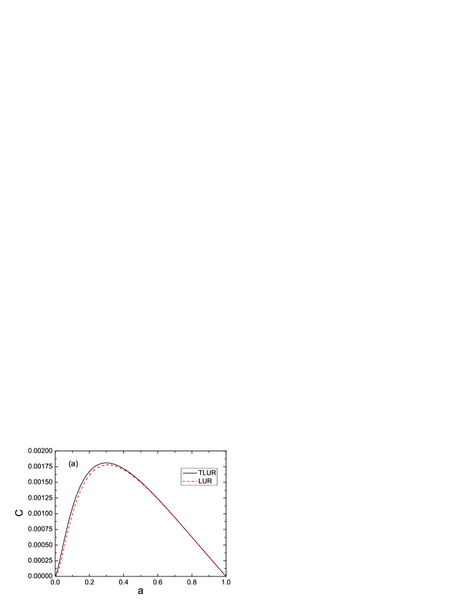
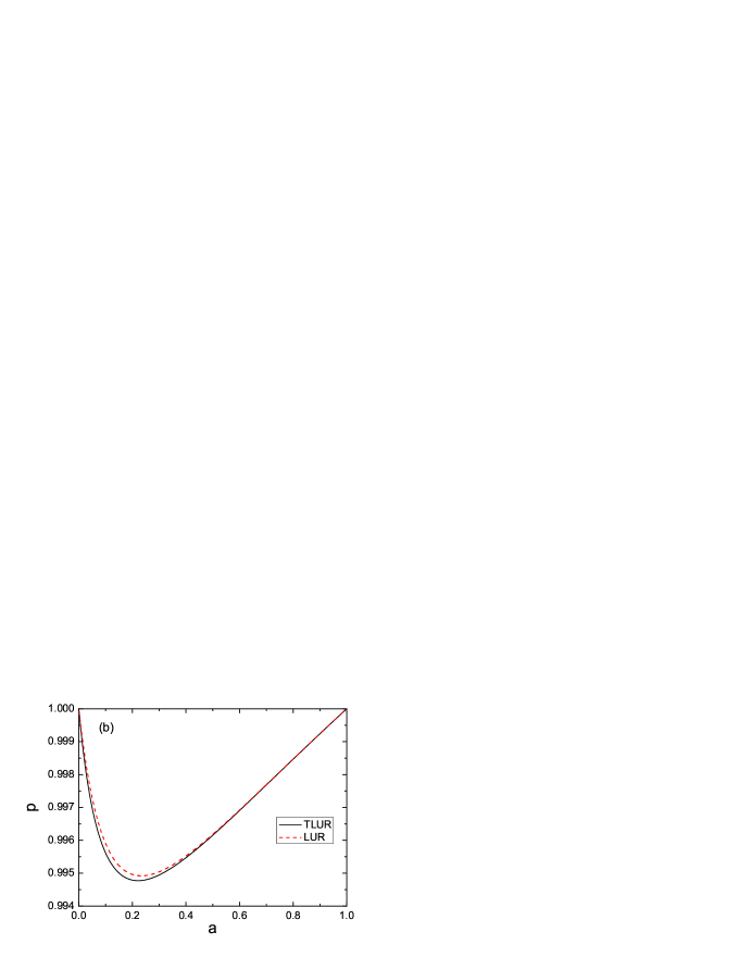
Figure 1: (color online). (a) Describing the amount of entanglement for Horodecki $3\times 3$ bound entangled state via $C_{TLUR}$ (solid line) and $C_{LUR}$ (dashed line). $C_{TLUR}$ is always larger than $C_{LUR}$. (b) Detecting the entanglement of Horodecki $3\times 3$ bound entangled state with white noise. The regions above the curves can be detected as entangled states by the TLUR criterion (solid line) and the original LUR criterion (dashed line), respectively.

Example 1.– To compare with the original LUR criterion, we consider the same example which has been used in Ref. LUR2 . P. Horodecki introduced a $3\times 3$ bound entangled state in Ref. bound , and its density matrix $\rho$ is real and symmetric as

$$\rho = \frac{a}{1+8a}\big{(}\mid-1;0\rangle\langle-1;0\mid+\mid-1;+1\rangle\langle-1;+1\mid$$

$$+\mid 0;-1\rangle\langle 0;-1\mid+\mid 0;+1\rangle\langle 0;+1\mid+\mid+1;0\rangle\langle+1;0\mid\big{)}$$

$$+\frac{3a}{1+8a}\mid E_{\mbox{max}}\rangle\langle E_{\mbox{max}}\mid+\frac{1}{1+8a}\mid\Pi\rangle\langle\Pi\mid,$$

where

$$\mid E_{\mbox{max}}\rangle=\frac{1}{\sqrt{3}}\left(\mid-1;-1\rangle+\mid 0;0\rangle+\mid+1;+1\rangle\right)$$

and

$$\mid\Pi\rangle=\sqrt{\frac{1+a}{2}}\mid+1;-1\rangle+\sqrt{\frac{1-a}{2}}\mid+1;+1\rangle.$$

The real parameter $a$ covers the range $0<a<1$. If one chooses the sets of local observables $\{\hat{\lambda}_{k}(1)\}_{k=1}^{8}$ and $\{\hat{\lambda}_{k}(2)\}_{k=1}^{8}$ introduced in Ref. LUR2 , the bound entangled state violates both the original LUR and the tighter LUR (TLUR) criterion. On the other hand, if we define $C_{TLUR}=1-[\sum_{k}\delta(\hat{A}_{k}\otimes\mathbbm{1}+\mathbbm{1}\otimes\hat{B}_{k})^{2}-M^{2}]/(U_{A}+U_{B})$ as Ref. LUR1 defined $C_{LUR}$, where $C_{TLUR}$ and $C_{LUR}$ provide quantitative estimates of the amount of entanglement verified by the violation of LURs, it can be discovered that $C_{TLUR}$ is always larger than $C_{LUR}$, which has been demonstrated in Fig. 1(a). Furthermore, let us consider a mixture of this state with white noise, $\rho(p)=p\rho+(1-p)\mathbbm{1}/9$. Taking the TLUR in Eq. (5) and the LUR in Eq. (3) with the Schmidt matrices of $\rho(p)$ as the set of local observables nonlinear , one finds that more entangled states can be detected by the TLUR criterion than by the LUR criterion. Detailed results are shown in Fig. 1(b).

III Relation with other criteria

In this section, we discuss the relation between Theorem 1 and some other entanglement conditions that have been proposed in the past. Actually, if we choose some special sets of local observables in Theorem 1, there are several corollaries that can be obtained in a form reduced to some other criteria or improved versions of them. One of them is derived from local orthogonal observables (LOOs) $\hat{G}_{k}^{A}$ and $\hat{G}_{k}^{B}$ which are orthogonal bases of the observable spaces $\mathcal{B}(\mathcal{H}_{A})$ and $\mathcal{B}(\mathcal{H}_{B})$ and satisfy $\mathrm{Tr}(\hat{G}_{k}^{A}\hat{G}_{l}^{A})=\mathrm{Tr}(\hat{G}_{k}^{B}\hat{G}_{l}^{B})=\delta_{kl}$.

Corollary 1. A stronger witness can be obtained from TLUR using complete sets of LOOs as the set of local observables,

$$1-\sum_{k}\langle\hat{G}_{k}^{A}\otimes\hat{G}_{k}^{B}\rangle-\frac{1}{2}\sum_{k}\langle\hat{G}_{k}^{A}\otimes\mathbbm{1}-\mathbbm{1}\otimes\hat{G}_{k}^{B}\rangle^{2}$$

$$-\frac{1}{2}\bigg{(}\sqrt{1-\mathrm{Tr}\rho_{A}^{2}}-\sqrt{1-\mathrm{Tr}\rho_{B}^{2}}\bigg{)}^{2}\geq 0,$$ (6)

Eq. (6) holds for all bipartite separable states.

Proof.– One can choose $\hat{A}_{k}=\hat{G}_{k}^{A}$, $\hat{B}_{k}=-\hat{G}_{k}^{B}$, and use $\sum_{k}\langle(\hat{G}_{k}^{A})^{2}\rangle=d_{A}$, $\sum_{k}\langle\hat{G}_{k}^{A}\rangle^{2}=\mathrm{Tr}\rho_{A}^{2}$, $\sum_{k}\langle(\hat{G}_{k}^{B})^{2}\rangle=d_{B}$, and $\sum_{k}\langle\hat{G}_{k}^{B}\rangle^{2}=\mathrm{Tr}\rho_{B}^{2}$, which have been shown in Ref. nonlinear , to obtain Corollary 1. $\square$

Remark. Corollary 1 is an improved version of the nonlinear witness introduced in Ref. nonlinear . Any entangled states, which can be detected by the original nonlinear witness nonlinear , $1-\sum_{k}\langle\hat{G}_{k}^{A}\otimes\hat{G}_{k}^{B}\rangle-\frac{1}{2}\sum_{k}\langle\hat{G}_{k}^{A}\otimes\mathbbm{1}-\mathbbm{1}\otimes\hat{G}_{k}^{B}\rangle^{2}\geq 0$, can also be detected by Corollary 1; the converse is not true in general.

It is worth noticing that Corollary 1 can be easily realized in experiments, since the left hand side of Eq. (6) can be directly measured ($\sum_{k}\langle\hat{G}_{k}^{A}\rangle^{2}=\mathrm{Tr}\rho_{A}^{2}$, $\sum_{k}\langle\hat{G}_{k}^{B}\rangle^{2}=\mathrm{Tr}\rho_{B}^{2}$). To show this, we will provide a short example in the following.

Example 2.– To compare with the original nonlinear witness, we consider the same example which has been used in Ref. nonlinear . Let us consider a noisy singlet state of the form

$$\rho(p)=p|\psi_{s}\rangle\langle\psi_{s}|+(1-p)\rho_{sep},$$ (7)

where $|\psi_{s}\rangle=(|01\rangle-|10\rangle)/\sqrt{2}$ and $\rho_{sep}=2/3|00\rangle\langle 00|+1/3|01\rangle\langle 01|$. Actually, $\rho(p)$ is entangled for any $p>0$ nonlinear . Now we choose $\hat{G}_{k}^{A}$ and $\hat{G}_{k}^{B}$ as

$$\{\hat{G}_{k}^{A}\}_{k=1}^{4} = \bigg{\{}-\frac{\sigma_{x}}{\sqrt{2}},-\frac{\sigma_{y}}{\sqrt{2}},-\frac{\sigma_{z}}{\sqrt{2}},\frac{\mathbbm{1}}{\sqrt{2}}\bigg{\}},$$

$$\{\hat{G}_{k}^{B}\}_{k=1}^{4} = \bigg{\{}\frac{\sigma_{x}}{\sqrt{2}},\frac{\sigma_{y}}{\sqrt{2}},\frac{\sigma_{z}}{\sqrt{2}},\frac{\mathbbm{1}}{\sqrt{2}}\bigg{\}}.$$ (8)

It can be seen that $\rho(p)$ voilates the original nonlinear witness for all $p>0.25$ nonlinear . Using Eq. (6) with these LOOs, one finds that $\rho(p)$ is entangled at least for $p>0.221$.

Besides Corollary 1, we can also obtain the conclusion that the CCNR criterion, the criterion based on Bloch representations, and the extension of CCNR criterion are the corollaries of Theorem 1. This is because these three criteria are the corollaries of the symmetric CMC criterion and that the symmetric CMC using orthogonal observables is equivalent to the LUR criterion.

It is worth noticing that Theorem 1 can also be used for continuous variables. If we choose $\{|a|\hat{x}_{1},|a|\hat{p}_{1}\}_{A}$ and $\{\hat{x}_{2}/a,-\hat{p}_{2}/a\}_{B}$ as the sets of local observables, and use $\langle(\Delta\hat{x}_{j})^{2}\rangle+\langle(\Delta\hat{p}_{j})^{2}\rangle\geq|[\hat{x}_{j},\hat{p}_{j}]|=1$ for $j=1,2$, the following corollary will be obtained from Theorem 1.

Corollary 2. For continuous variable systems, define $\hat{u}=|a|\hat{x}_{1}+\hat{x}_{2}/a$ and $\hat{v}=|a|\hat{p}_{1}-\hat{p}_{2}/a$ with $\hat{x}_{j}$ and $\hat{p}_{j^{\prime}}$ satisfying $[\hat{x}_{j},\hat{p}_{j^{\prime}}]=i\delta_{jj^{\prime}}$ ($j,j^{\prime}=1,2$). The inequality

$$\langle(\Delta\hat{u})^{2}\rangle+\langle(\Delta\hat{v})^{2}\rangle\geq a^{2}+\frac{1}{a^{2}}+M^{2}$$ (9)

holds for all separable states, where $M=|a|\sqrt{\langle(\Delta\hat{x}_{1})^{2}\rangle+\langle(\Delta\hat{p}_{1})^{2}\rangle-1}-\sqrt{\langle(\Delta\hat{x}_{2})^{2}\rangle+\langle(\Delta\hat{p}_{2})^{2}\rangle-1}/|a|$.

Remark. Corollary 2 is an improved version of the entanglement criterion introduced in Ref. Duan , which provided an inequality $\langle(\Delta\hat{u})^{2}\rangle+\langle(\Delta\hat{v})^{2}\rangle\geq a^{2}+1/a^{2}$ for separable states. Since a squared nonnegative term $M^{2}$ has been added in the right hand side of Eq. (9), corollary 2 is strictly stronger than the criterion shown in Ref. Duan .

There is another interesting relation between the TLUR criterion and the symmetric CMC using arbitrary observables. Notice that Refs. CM ; CM2 mainly discussed the symmetric CMC using orthogonal observables and concluded that the LUR criterion is equivalent to the symmetric CMC using orthogonal observables. Interestingly, if arbitrary local observables $\{\hat{A}_{k}\}$ and $\{\hat{B}_{k}\}$ are used, the TLUR can be obtained from the symmetric CMC otfried .

Proposition 1. The TLUR criterion is a corollary of the symmetric CMC using arbitrary local observables otfried .

Proof.— Using Eq. (43) of Ref. CM2 $\|C\|^{2}_{Tr}\leq\|A-\kappa_{A}\|_{Tr}\|B-\kappa_{B}\|_{Tr}$ where $\|\cdot\|_{Tr}$ is the trace norm (i.e., the sum of the singular values), $\kappa_{A}=\sum_{i}p_{i}\gamma^{S}(\rho_{i}^{A})$, $\kappa_{B}=\sum_{i}p_{i}\gamma^{S}(\rho_{i}^{B})$, and $\gamma^{S}$ stands for the symmetric covariance matrix, one can obtain that $[\sum_{k}(\langle\hat{A}_{k}\otimes\hat{B}_{k}\rangle-\langle\hat{A}_{k}\otimes\mathbbm{1}\rangle\langle\mathbbm{1}\otimes\hat{B}_{k}\rangle)]^{2}=(\mathrm{Tr}C)^{2}\leq\|C\|^{2}_{Tr}\leq\|A-\kappa_{A}\|_{Tr}\|B-\kappa_{B}\|_{Tr}=(\mathrm{Tr}A-\mathrm{Tr}\kappa_{A})(\mathrm{Tr}B-\mathrm{Tr}\kappa_{B})=[\sum_{k}\delta(\hat{A}_{k})_{\rho_{A}}^{2}-\sum_{i}p_{i}\sum_{k}\delta(\hat{A}_{k})_{\rho^{A}_{i}}^{2}][\sum_{k}\delta(\hat{B}_{k})_{\rho_{B}}^{2}-\sum_{i}p_{i}\sum_{k}\delta(\hat{B}_{k})_{\rho^{B}_{i}}^{2}]\leq[\sum_{k}\delta(\hat{A}_{k})_{\rho_{A}}^{2}-U_{A}][\sum_{k}\delta(\hat{B}_{k})_{\rho_{B}}^{2}-U_{B}]$, where $\sum_{k}\delta(\hat{A}_{k})_{\rho^{A}_{i}}^{2}\geq U_{A}$ and $\sum_{k}\delta(\hat{B}_{k})_{\rho^{B}_{i}}^{2}\geq U_{B}$ have been used. Therefore, Lemma 1 and Theorem 1 can be obtained from the symmetric CMC using arbitrary observables. $\square$

Remark. Refs. CM ; CM2 show that the LUR criterion using arbitrary observables is equivalent to the symmetric CMC using orthogonal observables. Obviously, the symmetric CMC using orthogonal observables is a corollary of the symmetric CMC using arbitrary observables. From Proposition 1, TLUR criterion is also a corollary of the symmetric CMC using arbitrary observables. However, whether the TLUR criterion is equivalent to the LUR criterion (the symmetric CMC using orthogonal observables) is unknown.

IV Discussion and conclusion

There are still several questions about the TLUR. First, Theorem 1 and the original LUR criterion are considered for bipartite systems. Is it possible to generalize them to multipartite systems? Second, we have shown that Theorem 1 is stronger than the LUR when the set of local observables is chosen. However, if one chooses all possible sets of local observables, is Theorem 1 still stronger than or just equivalent to the LUR criterion? Finally, for discrete variable systems, Theorem 1 can be used for detecting bound entangled states. Is it then possible to detect bound entangled states for continuous variables? These questions are interesting and worth for further research.

In summary, we have proposed an entanglement criterion based on the TLUR, which can be viewed as an extension of the original LUR criterion. Using arbitrarily chosen operators $\{\hat{A}_{k}\}$ and $\{\hat{B}_{k}\}$ of subsystems A and B, the TLUR criterion, which may be used not only for discrete variables but also for continuous variables, can detect more entangled states than the LUR criterion since a nonnegative term has been added, similar to the nonlinear witnesses.

APPENDIX

Here we prove Lemma 1. The density matrix for bipartite separable states can be expressed as $\rho_{AB}=\sum_{i}p_{i}\rho_{i}^{A}\otimes\rho_{i}^{B}$. Notice that the lemma is equivalent to

$$[\sum_{k}\delta(\hat{A}_{k})_{\rho_{A}}^{2}-U_{A}][\sum_{k}\delta(\hat{B}_{k})_{\rho_{B}}^{2}-U_{B}]$$

$$\geq[\sum_{k}(\langle\hat{A}_{k}\otimes\hat{B}_{k}\rangle-\langle\hat{A}_{k}\otimes\mathbbm{1}\rangle\langle\mathbbm{1}\otimes\hat{B}_{k}\rangle)]^{2}.$$ (10)

The right hand side (RHS) and the left hand side (LHS) of Eq. (10) can be written as

$$\mathrm{RHS}$$

$$= \{\sum_{k}[\sum_{i}p_{i}\langle\hat{A}_{k}\rangle_{i}\langle\hat{B}_{k}\rangle_{i}-(\sum_{i}p_{i}\langle\hat{A}_{k}\rangle_{i})(\sum_{i^{\prime}}p_{i^{\prime}}\langle\hat{B}_{k}\rangle_{i^{\prime}})]\}^{2}$$

$$= \{\sum_{k}\sum_{i}p_{i}\langle(\hat{A}_{k}-\sum_{i^{\prime}}p_{i^{\prime}}\langle\hat{A}_{k}\rangle_{i^{\prime}})\rangle_{i}\langle(\hat{B}_{k}-\sum_{j^{\prime}}p_{j^{\prime}}\langle\hat{B}_{k}\rangle_{j^{\prime}})\rangle_{i}\}^{2}$$

$$\equiv \{\sum_{k}\sum_{i}p_{i}\langle\mathfrak{A}_{k}\rangle_{i}\langle\mathfrak{B}_{k}\rangle_{i}\}^{2},$$

where we have defined $\langle\hat{A}_{k}\rangle_{i}=\langle\hat{A}_{k}\rangle_{\rho_{i}^{A}}$, $\langle\hat{B}_{k}\rangle_{i}=\langle\hat{B}_{k}\rangle_{\rho_{i}^{B}}$, $\mathfrak{A}_{k}=\hat{A}_{k}-\sum_{i^{\prime}}p_{i^{\prime}}\langle\hat{A}_{k}\rangle_{i^{\prime}}$ and $\mathfrak{B}_{k}=\hat{B}_{k}-\sum_{j^{\prime}}p_{j^{\prime}}\langle\hat{B}_{k}\rangle_{j^{\prime}}$ for convenience. Therefore,

$$\mathrm{LHS}$$

$$= (\sum_{k}\sum_{i}p_{i}\langle(\mathfrak{A}_{k})^{2}\rangle_{i}-U_{A})(\sum_{k}\sum_{i}p_{i}\langle(\mathfrak{B}_{k})^{2}\rangle_{i}-U_{B})$$

$$\geq (\sum_{k}\sum_{i}p_{i}\langle\mathfrak{A}_{k}\rangle_{i}^{2})(\sum_{k}\sum_{i}p_{i}\langle\mathfrak{B}_{k}\rangle_{i}^{2}),$$

where we have used $\sum_{k}\sum_{i}p_{i}(\langle(\mathfrak{A}_{k})^{2}\rangle_{i}-\langle\mathfrak{A}_{k}\rangle_{i}^{2})=\sum_{k}\sum_{i}p_{i}(\langle(A_{k})^{2}\rangle_{i}-\langle A_{k}\rangle_{i}^{2})\geq U_{A}$ and $\sum_{k}\sum_{i}p_{i}(\langle(\mathfrak{B}_{k})^{2}\rangle_{i}-\langle\mathfrak{B}_{k}\rangle_{i}^{2})=\sum_{k}\sum_{i}p_{i}(\langle(B_{k})^{2}\rangle_{i}-\langle B_{k}\rangle_{i}^{2})\geq U_{B}$.

With the help of the Cauchy-Schwarz inequality, it can be obtained that

$$\mathrm{LHS} \geq (\sum_{k}\sum_{i}p_{i}\langle\mathfrak{A}_{k}\rangle_{i}^{2})(\sum_{k}\sum_{i}p_{i}\langle\mathfrak{B}_{k}\rangle_{i}^{2})$$

$$\geq (\sum_{k}\sum_{i}p_{i}\langle\mathfrak{A}_{k}\rangle_{i}\langle\mathfrak{B}_{k}\rangle_{i})^{2}$$

$$= \mathrm{RHS}.$$

Therefore, Lemma 1 has been proved. $\square$

References

• (1) M. A. Nielsen and I. L. Chuang, Quantum Computation and Quantum Information (Cambridge University Press, Cambridge, 2000).
• (2) D. Leibfried, E. Knill, S. Seidelin, J. Britton, R. B. Blakestad, J. Chiaverini, D. B. Hume, W. M. Itano, J. D. Jost, C. Langer, R. Ozeri, R. Reichle, and D. J. Wineland, Nature 438, 639 (2005).
• (3) H. Häffner, W. Hänsel, C. F. Roos, J. Benhelm, D. Chek-al-kar, M. Chwalla, T. Körber, U. D. Rapol, M. Riebe, P. O. Schmidt, C. Becher, O. Gühne, W. Dür, and R. Blatt, Nature 438, 643 (2005).
• (4) C.-Y. Lu, X.-Q. Zhou, O. Gühne, W.-B. Gao, J. Zhang, Z.-S. Yuan, A. Goebel, T. Yang and J.-W. Pan, Nature Phys. 3, 91 (2007).
• (5) R. F. Werner, Phys. Rev. A 40, 4277 (1989).
• (6) D. Bruß, J. Math. Phys. 43, 4237 (2002); M. B. Plenio, S. Virmani, Quantum Inf. Comput. 7, 1 (2007); R. Horodecki, P. Horodecki, M. Horodecki, and K. Horodecki, Rev. Mod. Phys. 81, 865 (2009); O. Gühne and G. Tóth, Phys. Rep. 474, 1 (2009).
• (7) A. Peres, Phys. Rev. Lett. 77, 1413 (1996); M. Horodecki, P. Horodecki, and R. Horodecki, Phys. Lett. A 223, 1 (1996).
• (8) H. F. Hofmann and S. Takeuchi, Phys. Rev. A 68, 032103 (2003).
• (9) H. F. Hofmann, Phys. Rev. A 68, 034307 (2003).
• (10) O. Gühne, P. Hyllus, O. Gittsovich, and J. Eisert, Phys. Rev. Lett. 99, 130504 (2007).
• (11) O. Gittsovich, O. Gühne, P. Hyllus, and J. Eisert, Phys. Rev. A 78, 052319 (2008).
• (12) O. Rudolph, arXiv:quant-ph/0202121.
• (13) K. Chen and L.-A. Wu, Quantum Inf. Comput. 3, 193 (2003).
• (14) M. Horodecki, P. Horodecki, and R. Horodecki, Open Syst. Inf. Dyn. 13, 103 (2006).
• (15) H. Fan, arXiv:quant-ph/0210168; P. Wocjan, M. Horodecki, Open Syst. Inf. Dyn. 12, 331 (2005); L. Clarisse, P. Wocjan, Quantum Inf. Comput. 6, 277 (2006).
• (16) J.I. de Vicente, Quantum Inf. Comput. 7, 624 (2007); J.I. de Vicente, J. Phys. A 41, 065309 (2008).
• (17) B. Terhal, Phys. Lett. A 271, 319 (2000); G. Tóth and O. Gühne, Phys. Rev. Lett. 94, 060501 (2005); F. A. Bovino, G. Castagnoli, A. Ekert, P. Horodecki, C. M. Alves and A. V. Sergienko, Phys. Rev. Lett. 95, 240407 (2005); O. Gühne, G. Tóth, P. Hyllus, and H. J. Briegel, ibid. 95, 120405 (2005); F. Mintert, Phys. Rev. A 75, 052302 (2007); R. Augusiak, M. Demianowicz, P. Horodecki, ibid. 77, 030301(R) (2008).
• (18) O. Gühne and N. Lütkenhaus, Phys. Rev. Lett. 96, 170502 (2006);
• (19) C.-J. Zhang, Y.-S. Zhang, S. Zhang, and G.-C. Guo, Phys. Rev. A 77, 060301(R) (2008).
• (20) O. Gühne, Phys. Rev. Lett. 92, 117903 (2004).
• (21) G. Tóth, C. Knapp, O. Gühne, and H. J. Briegel, Phys. Rev. Lett. 99, 250405 (2007); G. Tóth, C. Knapp, O. Gühne, and H. J. Briegel, Phys. Rev. A 79, 042334 (2009).
• (22) G. Tóth,and O. Gühne, Phys. Rev. Lett. 102, 170503 (2009); G. Tóth, W. Wieczorek, R. Krischek, N. Kiesel, P. Michelberger, and H. Weinfurter, New J. Phys. 11, 083002 (2009).
• (23) O. Gühne, M. Mechler, G. Tóth, and P. Adam, Phys. Rev. A 74, 010301(R) (2006).
• (24) S. Yu and N.-L. Liu, Phys. Rev. Lett. 95, 150504 (2005).
• (25) P. Aniello and C. Lupo, J. Phys. A: Math. Theor. 41, 355303 (2008); C. Lupo, P. Aniello, and A. Scardicchio, ibid. 41, 415301 (2008).
• (26) O. Gühne amd M. Seevinck, arXiv:0905.1349.
• (27) R. Augusiak and J. Stasińska, New J. Phys. 11, 053018 (2009).
• (28) W. K. Wootters, Phys. Rev. Lett. 80, 2245 (1998); A. Uhlmann, Phys. Rev. A 62, 032307 (2000); P. Rungta, V. Bužek, C. M. Caves, M. Hillery and G. J. Milburn, Phys. Rev. A 64, 042315 (2001).
• (29) H. Fan, K. Matsumoto and H. Imai, J. Phys. A 36, 4151 (2003); H. Fan, V. Korepin, and V. Roychowdhury, Phys. Rev. Lett. 93, 227203 (2004).
• (30) F. Mintert, M. Kuś and A. Buchleitner, Phys. Rev. Lett. 92, 167902 (2004); H. P. Breuer, J. Phys. A 39, 11847 (2006); J.I. de Vicente, Phys. Rev. A 75, 052320 (2007).
• (31) K. Chen, S. Albeverio and S.-M. Fei, Phys. Rev. Lett. 95, 040504 (2005); K. Chen, S. Albeverio and S.-M. Fei, ibid. 95, 210501 (2005).
• (32) M. Li, S.-M. Fei, and Z.-X. Wang, J. Phys. A 41, 202002 (2008); M.-J. Zhao, Z.-X. Wang, and S.-M. Fei, Rep. Math. Phys. 63, 409 (2009); S.-M. Fei, M.-J. Zhao, K. Chen, and Z.-X. Wang, Phys. Rev. A 80, 032320 (2009).
• (33) Z.-H. Ma, F.-L. Zhang, D.-L. Deng, and J.-L. Chen, Phys. Lett. A 373, 1616 (2009); Z.-H. Ma, F.-L. Zhang, and J.-L. Chen, Phys. Rev. A 78, 064305 (2008).
• (34) R. Simon, Phys. Rev. Lett. 84, 2726 (2000).
• (35) L.-M. Duan, G. Giedke, J. I. Cirac, and P. Zoller, Phys. Rev. Lett. 84, 2722 (2000).
• (36) R. F. Werner and M. M. Wolf, Phys. Rev. Lett. 86, 3658 (2001).
• (37) G. Giedke, B. Kraus, M. Lewenstein, and J. I. Cirac, Phys. Rev. Lett. 87, 167904 (2001).
• (38) H. Nha, and M. S. Zubairy, Phys. Rev. Lett. 101, 130402 (2008); Q. Sun, H. Nha, and M. S. Zubairy, Phys. Rev. A 80, 020101(R) (2009).
• (39) P. Horodecki, Phys. Lett. A 232, 333 (1997).
• (40) O. Gühne, Private communication.