Non-linear waves in a Quark Gluon Plasma

Abstract

Recent measurements at RHIC suggest that a nearly perfect fluid of quarks and gluons is produced in $A\,A$ collisions. Moreover the passage of supersonic partons through this medium seems to produce waves. These waves might pile up and form Mach cones, which would manifest themselves in the so called away-side jets, forming a broad structure in the angular distribution of the particles recoiling against a trigger jet of moderate energy. In most of the theoretical descriptions of these phenomena, the hydrodynamic equations are linearized for simplicity. We propose an alternative explanation for the observed broadening of the away-side peak. It is based on hydrodynamics but it is a consequence of the non-linearities of the equations, which instead of simple waves may lead to localized waves or even solitons.

We investigate in detail the consequences of including the non-linear terms. We use a simple equation of state for the QGP and expand the hydrodynamic equations around equilibrium configurations. The resulting differential equations describe the propagation of perturbations in the energy density. We solve them numerically and find that localized perturbations can propagate for long distances in the plasma. Under certain conditions our solutions mimick the propagation of Korteweg - de Vries solitons.

I Introduction

The heavy ion collisions performed at BNL’s Relativistic heavy Ion Collider (RHIC) create a hot and dense medium, which behaves as a perfect fluid. During the first years of the RHIC program, hydrodynamics was applied to describe the space-time evolution of the bulk of the fluid. In the last years hydrodynamics became relevant to study also the perturbations on the fluid, such as, for example, the waves generated by the passage of a supersonic parton. This field was opened by the observation of a broad structure in azimuthal di-hadron correlations star ; phenix . This broad structure is called the “away-side jet” and recoils against the “near-side jet” (or “trigger jet”). In the framework of hydrodynamics, this observation could be explained by the conical shock waves generated by large energy deposition in the hydrodynamical medium ma1 ; ma2 ; ma3 ; ma4 ; ma5 ; ma6 ; ma7 ; ma8 ; ma9 ; betz1 ; betz2 ; betz3 . Although quite elegant, this understanding of the away-side jet in terms of conical shock waves still needs confirmation. A very recent and improved analysis by the STAR collaboration has given further support to this picture star09 . A more solid evidence of this phenomenon may come from the study of jets at the Large Hadron Colider (LHC), where the energy released by the nuclear projectiles in the central rapidity region will be larger dnw and so the formed fireball will be larger and live longer, allowing for a more complete study of waves.

In this work we discuss another possible mechanism for the formation of broad structures in the away-side jet. In the limit where the jet looses most of its energy, which is rapidly thermalized and incorporated to fluid, a pulse is formed, which propagates through the fluid. During its motion this energy density pulse spreads both in the longitudinal and transverse direction. After hadronization this travelling and expanding “hot spot” will form particles with a broader angular distribution than those coming from the near-side jet. This is depicted in Fig. 1. Notice that in this process there is no Mach cone formation. During the motion of the energy density pulse, the medium undergoes an expansion leading to a spread of this pulse. A further spreading will occur during the hadronization and final particle formation. Therefore, in this picture it is essential that the initial perturbation remains localized to a good extent. Otherwise it will spread too much and destroy the jet-like topology, which is compatible with data.

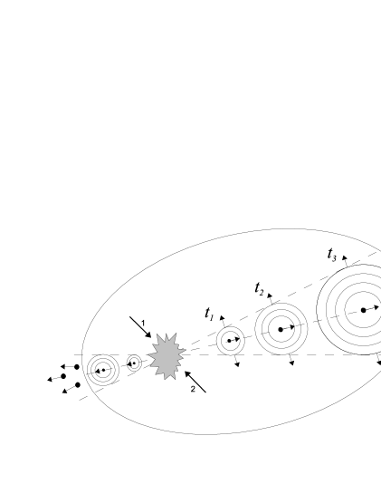
Figure 1: Parton-parton collision forming two back-to-back jets, which evolve in a hot quark gluon plasma. The circles represent localized (soliton-like) energy density perturbations which traverse the fluid and suffer expansion, forming a narrow near-side jet and a broad away-side jet.

Highly localized perturbations can exist and propagate through a fluid. The most famous are the Korteweg - de Vries (KdV) solitons, which are solutions of the KdV equation. This equation may be derived from the equations of hydrodynamics under certain conditions. One of them is to preserve the non-linear terms of the Euler and continuity equations. The other one is to have a third order spatial derivative term. This term comes from the equation of state of the fluid and it appears because the Lagrangian density contains higher derivative couplings fn1 ; fn2 ; fn3 or because of the Laplacians appearing in the equations of motion of the fields of the theory fn4 . This happens, for example, in the non-linear Walecka model of nuclear matter at zero and finite temperature. For a quark gluon plasma (QGP) it depends on the coupling regime and on the properties of the QCD vacuum. As it will be seen in this work, if we consider the simplest case of a free gas of massless quarks and gluons, the hydrodynamical equations do not give origin to the KdV equation. Instead they generate a non-linear differential equation for the perturbation which has no third order stabilising term. This equation is called wave breaking equation and is also very well knonw in the literature. The numerical solution of this equation shows that an initial gaussian-like perturbation in the energy density evolves creating a vertical “wall” in its front, which breaks and looses localization. In our case, surprisingly enough, this same phenomenon happens but it takes a very long time and long distances, compared to the nuclear scales. So, from the practical point of view, there is no distinction between a breaking pulse and a soliton. This persistence of localization in the breaking wave is the main result of our paper and gives support to the process shown in Fig. 1. However, from this finding to a realistic calculation and a serious attempt to describe the data there is still a long way. The next step now will be to quantify the broadening of the moving bubble in Fig. 1, which will be directly reflected in the angular distribution of the fragments. For this we need to extend our formalism to two spatial dimensions (longitudinal $x$ and radial $r$). This is a heavily numerical project and it is still in progress. Based on previous works with the analogous non-relativistic problem for nuclear matter, discussed in rww , we have reasons to expect a soliton-like evolution along the $x$ direction with a “leakage” to the radial direction, which would cause the angular broadening in the final matter distribution.

In the theoretical description of these perturbations ma2 ; ma8 ; ma9 , very often the hydrodynamic equations are linearized for simplicity. As it is usually done in non-relativistic hydrodynamics, linearization consists hidro1 in considering only first order terms in the velocity and in the energy and pressure perturbations and neglecting higher order terms and derivatives involving them. In this work we revisit the relativistic hydrodynamic equations expanding them in a different way, in terms of a small expansion parameter ($\sigma$) closely following what is done in magnetohydrodynamics of plasmas davidson and keeping the non-linear features of the problem. Techniques of plasma physics started to be applied to nuclear hydrodynamics long ago frsw ; abu to study perturbations in the cold nucleus, treated as a fluid. We extended those pioneering studies to relativistic and warm nuclear matter fn1 ; fn2 ; fn3 ; fn4 and now to the quark gluon plasma (QGP).

The most interesting aspect of frsw ; abu ; fn1 ; fn2 ; fn3 ; fn4 was to find at some point of the developement, the (KdV) equation for the perturbation in the nuclear matter density. This is the “nuclear soliton”. Our main contribution was to establish a connection between the KdV equation (and the properties of its solitonic solutions) and a modern underlying nuclear matter theory (which in our case was a variant of the non-linear Walecka model) and then to show that the soliton solution exists even in relativistic hydrodynamics fn1 ; fn2 .

In the next section we review the main formulas of relativistic hydrodynamics. In section III we discuss the quark gluon plasma equation of state. In sections IV and V we show how to derive the diffferential equations which govern the time evolution of perturbations at zero and finite temperature respectively. In section VI we present the numerical solutions of the obtained differential equations and in section VII we present some conclusions.

II Relativistic Fluid Dynamics

In this section we review the main expressions of one dimensional relativistic hydrodynamics. Throughout this work we employ natural units $c=1$, $\hbar=1$ and (Boltzmann’s constant) $k_{B}=1$. The velocity four vector $u^{\nu}$ is defined as $u^{0}=\gamma$, $\vec{u}=\gamma\vec{v}$, where $\gamma$ is the Lorentz factor given by $\gamma=(1-v^{2})^{-1/2}$ and thus $u^{\nu}u_{\nu}=1$. The velocity field of the matter is $\vec{v}=\vec{v}(t,x,y,z)$. The energy-momentum tensor is, as usual, given by:

$$T_{\mu\nu}=(\varepsilon+p)u_{\mu}u_{\nu}-pg_{\mu\nu}$$ (1)

where $\varepsilon$ and $p$ are the energy density and pressure respectively. Energy-momentum conservation is ensured by:

$$\partial_{\nu}{T_{\mu}}^{\nu}=0$$ (2)

The projection of (2) onto a direction perpendicular to $u^{\mu}$ gives the relativistic version of the Euler equation wein ; land :

$${\frac{\partial{\vec{v}}}{\partial t}}+(\vec{v}\cdot\vec{\nabla})\vec{v}=-{\frac{1}{(\varepsilon+p)\gamma^{2}}}\bigg{(}{\vec{\nabla}p+\vec{v}{\frac{\partial p}{\partial t}}}\bigg{)}$$ (3)

The relativistic version of the continuity equation for the baryon density is wein :

$$\partial_{\nu}{j_{B}}^{\nu}=0$$ (4)

Since ${j_{B}}^{\nu}=u^{\nu}\rho_{B}$ the above equation can be rewritten as:

$${\frac{\partial\rho_{B}}{\partial t}}+\gamma^{2}v\rho_{B}\Bigg{(}{\frac{\partial v}{\partial t}}+\vec{v}\cdot\vec{\nabla}v\Bigg{)}+\vec{\nabla}\cdot(\rho_{B}\vec{v})=0$$ (5)

The relativistic version of the continuity equation for the entropy density is given by the projection of (2) onto the direction of $u^{\nu}$ land :

$$(\varepsilon+p)\partial_{\mu}u^{\mu}+u^{\mu}\partial_{\mu}\varepsilon=0$$ (6)

At this point we recall the Gibbs relation:

$$\varepsilon+p={\mu_{B}}{\rho_{B}}+Ts$$ (7)

and the first law of thermodynamics:

$$d\varepsilon=Tds+{\mu_{B}}d{\rho_{B}}$$ (8)

We will later consider a hot gas of quarks and gluons, where the net baryon density is zero, i.e., $\rho_{B}=0$ ($d\rho_{B}=0$) at $T\neq 0$. Using this last relation in (8) and then inserting (8) and (7) in (6) we arrive at

$$Ts(\partial_{\mu}u^{\mu})+Tu^{\mu}(\partial_{\mu}s)=0$$

and finally at

$$\partial_{\nu}(s{u}^{\nu})=0$$ (9)

which was expected for a perfect fluid. For future use, the above formula will be expanded as:

$${\frac{\partial s}{\partial t}}+\gamma^{2}vs\Bigg{(}{\frac{\partial v}{\partial t}}+\vec{v}\cdot\vec{\nabla}v\Bigg{)}+\vec{\nabla}\cdot(s\vec{v})=0$$ (10)

which is quite similar to (5).

III The QGP Equation of State

We shall use a simple equation of state derived from the MIT Bag Model. It describes an ideal gas of quarks and gluons and takes into account the effects of confinement through the bag constant $\mathcal{B}$. This constant is interpreted as the energy needed to create a bubble or bag in the vacuum (in which the noninteracting quarks and gluons are confined) and it can be extracted from hadron spectroscopy or from lattice QCD calculations. There is a relationship between $\mathcal{B}$ and the critical temperature of the quark-hadron transition $T_{c}$ which is determined by assuming that, during the phase transition, the pressure vanishes.

The baryon density is given by:

$$\rho_{B}={\frac{1}{3}}{\frac{\gamma_{Q}}{(2\pi)^{3}}}\int d^{3}{k}\hskip 5.69046pt[n_{\vec{k}}-\bar{n}_{\vec{k}}]$$ (11)

where

$$n_{\vec{k}}\equiv n_{\vec{k}}(T)={\frac{1}{1+e^{(k-{\frac{1}{3}}\mu)/T}}}$$ (12)

and

$$\bar{n}_{\vec{k}}\equiv\bar{n}_{\vec{k}}(T)={\frac{1}{1+e^{(k+{\frac{1}{3}}\mu)/T}}}$$ (13)

where from now on $\mu$ is the baryon chemical potential. At zero temperature the expression for the baryon density reduces to:

$${\rho_{B}}={\frac{2}{3\pi^{2}}}{k_{F}}^{3}$$ (14)

where $k_{F}$ is the highest occupied level. The energy density and the pressure are given by:

$$\varepsilon=\mathcal{B}+{\frac{\gamma_{G}}{(2\pi)^{3}}}\int d^{3}{k}\hskip 5.69046ptk\hskip 5.69046pt(e^{k/T}-1)^{-1}+{\frac{\gamma_{Q}}{(2\pi)^{3}}}\int d^{3}{k}\hskip 5.69046ptk\hskip 5.69046pt[n_{\vec{k}}+\bar{n}_{\vec{k}}]$$ (15)

and

$$p=-\mathcal{B}+{\frac{1}{3}}\Bigg{\{}{\frac{\gamma_{G}}{(2\pi)^{3}}}\int d^{3}{k}\hskip 5.69046ptk\hskip 5.69046pt(e^{k/T}-1)^{-1}+{\frac{\gamma_{Q}}{(2\pi)^{3}}}\int d^{3}k\hskip 2.84544ptk\bigg{[}{n}_{\vec{k}}+\bar{n}_{\vec{k}}\bigg{]}\Bigg{\}}$$ (16)

The statistical factors are $\gamma_{G}=2\textrm{(polarizations)}\times 8\textrm{(colors)}=16$ for gluons and $\gamma_{Q}=2\textrm{(spins)}\times 2\textrm{(flavors)}\times 3\textrm{(colors)}=12$ for quarks. From the above expressions we derive the useful formulas:

$$3(p+\mathcal{B})=\varepsilon-\mathcal{B}={\frac{8\pi^{2}}{15}}\ T^{4}+{\frac{6}{\pi^{2}}}\int_{0}^{\infty}d{k}\hskip 5.69046ptk^{3}[n_{\vec{k}}+\bar{n}_{\vec{k}}]$$ (17)

and

$$p={\frac{1}{3}}\varepsilon-{\frac{4}{3}}\mathcal{B}$$ (18)

The speed of sound, $c_{S}$, is given by

$${c_{S}}^{2}={\frac{\partial p}{\partial\varepsilon}}={\frac{1}{3}}$$ (19)

IV Wave equation at zero temperature

In the core of a dense star the temperature is close to zero and the baryon density is very high. The quark distribution function becomes the step function. Using (14) in (15) and (16) we find:

$$\varepsilon(\rho_{B})=\bigg{(}{\frac{3}{2}}\bigg{)}^{7/3}\pi^{2/3}{\rho_{B}}^{4/3}+\mathcal{B}$$ (20)

and

$$p(\rho_{B})={\frac{1}{3}}\bigg{(}{\frac{3}{2}}\bigg{)}^{7/3}\pi^{2/3}{\rho_{B}}^{4/3}-\mathcal{B}$$ (21)

From (18) we have $\vec{\nabla}p={\frac{1}{3}}\vec{\nabla}\varepsilon$ and also ${\frac{\partial p}{\partial t}}={\frac{1}{3}}{\frac{\partial\varepsilon}{\partial t}}$. Combining these expressions with (20) and (21) we find:

$$\vec{\nabla}p={\frac{4}{9}}\bigg{(}{\frac{3}{2}}\bigg{)}^{7/3}\pi^{2/3}{\rho_{B}}^{1/3}\ \vec{\nabla}{\rho_{B}}$$ (22)

and

$${\frac{\partial p}{\partial t}}={\frac{4}{9}}\bigg{(}{\frac{3}{2}}\bigg{)}^{7/3}\pi^{2/3}{\rho_{B}}^{1/3}\ {\frac{\partial{\rho_{B}}}{\partial t}}$$ (23)

Finally, substituting (20), (21), (22) and (23) into (3) we obtain:

$${\rho_{B}}\bigg{[}{\frac{\partial{\vec{v}}}{\partial t}}+(\vec{v}\cdot\vec{\nabla})\vec{v}\bigg{]}=\frac{(v^{2}-1)}{3}\bigg{[}\vec{\nabla}{\rho_{B}}+\vec{v}{\frac{\partial{\rho_{B}}}{\partial t}}\bigg{]}$$ (24)

which is the relativistic version of Euler equation for the QGP at $T=0$.

Following the same formalism already used for nuclear matter in fn1 ; fn2 ; fn3 ; fn4 we will now expand both (5) and (24) in powers of a small parameter $\sigma$ and combine these two equations to find one single differential equation which governs the space-time evolution of the perturbation in the baryon density. We write (5) and (24) in one cartesian dimension ($x$) in terms of the dimensionless variables:

$$\hat{\rho}={\frac{\rho_{B}}{\rho_{0}}}\hskip 5.69046pt,\hskip 14.22636pt\hat{v}={\frac{v}{c_{S}}}$$ (25)

where $\rho_{0}$ is an equilibrium (or reference) density, upon which perturbations may be generated. Next, we introduce the $\xi$ and $\tau$ “stretched” coordinates frsw ; abu ; davidson :

$$\xi=\sigma^{1/2}{\frac{(x-{c_{S}}t)}{R}}\hskip 5.69046pt,\hskip 14.22636pt\tau=\sigma^{3/2}{\frac{{c_{S}}t}{R}}$$ (26)

After this change of variables we expand (25) as:

$$\hat{\rho}=1+\sigma\rho_{1}+\sigma^{2}\rho_{2}+\dots$$ (27)

$$\hat{v}=\sigma v_{1}+\sigma^{2}v_{2}+\dots$$ (28)

Neglecting terms proportional to $\sigma^{n}$ for $n\geq 3$ and organizing the equations as series in powers of $\sigma$, (5) and (24) aquire the form:

$$\sigma\Bigg{\{}{\frac{\partial\rho_{1}}{\partial\xi}}-{\frac{\partial v_{1}}{\partial\xi}}\Bigg{\}}+\sigma^{2}\Bigg{\{}{\frac{\partial v_{2}}{\partial\xi}}-{\frac{\partial\rho_{2}}{\partial\xi}}+{\frac{\partial\rho_{1}}{\partial\tau}}+\rho_{1}{\frac{\partial v_{1}}{\partial\xi}}+v_{1}{\frac{\partial\rho_{1}}{\partial\xi}}-{c_{S}}^{2}v_{1}{\frac{\partial v_{1}}{\partial\xi}}\Bigg{\}}=0$$

and

$$\sigma\Bigg{\{}{\frac{1}{3{c_{S}}^{2}}}{\frac{\partial\rho_{1}}{\partial\xi}}-{\frac{\partial v_{1}}{\partial\xi}}\Bigg{\}}+\sigma^{2}\Bigg{\{}-{\frac{\partial v_{2}}{\partial\xi}}+{\frac{1}{3{c_{S}}^{2}}}{\frac{\partial\rho_{2}}{\partial\xi}}+{\frac{\partial v_{1}}{\partial\tau}}+v_{1}{\frac{\partial v_{1}}{\partial\xi}}-2\rho_{1}{\frac{\partial v_{1}}{\partial\xi}}-{\frac{v_{1}}{3}}{\frac{\partial\rho_{1}}{\partial\xi}}+{\frac{\rho_{1}}{3{c_{S}}^{2}}}{\frac{\partial\rho_{1}}{\partial\xi}}\Bigg{\}}=0$$

respectively. In these equations each bracket must vanish independently, i.e. $\{\dots\}=0$. From the terms proportional to $\sigma$ we obtain ${c_{S}}^{2}=1/3$ and $\rho_{1}=v_{1}$, which are then inserted into the terms proportional to $\sigma^{2}$ giving after some algebra:

$${\frac{\partial\rho_{1}}{\partial\tau}}+{\frac{2}{3}}\rho_{1}{\frac{\partial\rho_{1}}{\partial\xi}}=0$$ (29)

Returning to the $x-t$ space the above equation reads:

$${\frac{\partial\hat{\rho}_{1}}{\partial t}}+c_{S}{\frac{\partial\hat{\rho}_{1}}{\partial x}}+{\frac{2}{3}}c_{S}\hat{\rho}_{1}{\frac{\partial\hat{\rho}_{1}}{\partial x}}=0$$ (30)

where we have used the notation $\hat{\rho}_{1}\equiv\sigma\rho_{1}$, which is a small perturbation in the baryon density. The equation (30) is the so called breaking wave equation for $\hat{\rho}_{1}$ at zero temperature in the QGP.

V Wave equation at finite temperature

In the central rapidity region of a typical heavy ion collision at RHIC we have a vanishing net baryon number, i.e., $\rho_{B}=0$. The energy is mostly stored in the gluon field, which forms the hot and dense medium. We will now aply hydrodynamics to study this medium and focus on perturbations in the energy density and their propagation. Following the formalism developed in the previous section we will expand and combine the Euler equation given by (3) and the continuity equation for the entropy density given by (10).

As $\rho_{B}=0$, the baryon chemical potential is zero $(\mu=0)$ and so the distribution functions given by (12) and (13) are the same, i.e. : ${n}_{\vec{k}}=\bar{n}_{\vec{k}}={1}/{(1+e^{k/T})}$. In this case the integral in (17) can be easily performed and we obtain:

$$3(p+\mathcal{B})=\varepsilon-\mathcal{B}={\frac{37}{30}}\pi^{2}T^{4}$$ (31)

Solving the first identity for the pressure and recalling reif that $s=({{\partial p}/{\partial T}})_{V}$ we arrive at:

$$s={\frac{\partial}{\partial T}}\bigg{(}-\mathcal{B}+{\frac{37}{90}}\pi^{2}T^{4}\bigg{)}=4\\ {\frac{37}{90}}\pi^{2}T^{3}$$ (32)

The “bag constant” parameter, $\mathcal{B}$, can be replaced by the critical temperature of the quark-hadron transition $T_{c}$. When $p=0$ at the phase transition, (31) reduces to:

$$\mathcal{B}={\frac{37}{90}}\pi^{2}(T_{c})^{4}$$ (33)

Inserting the above equation into the second identity of (31) we have the following expression for $\varepsilon(T)$:

$$\varepsilon={\frac{37}{30}}\pi^{2}\Bigg{(}T^{4}+{\frac{{T_{c}}^{4}}{3}}\Bigg{)}$$

From this formula we can define the reference energy density $\varepsilon_{0}$, which is related to a reference temperature, $T_{0}$, through:

$$\varepsilon_{0}={\frac{37}{30}}\pi^{2}\Bigg{(}{T_{0}}^{4}+{\frac{{T_{c}}^{4}}{3}}\Bigg{)}$$ (34)

Solving the second identity of (31) for the temperature we obtain:

$$T=\Bigg{[}{\frac{30}{37\pi^{2}}}(\varepsilon-\mathcal{B})\Bigg{]}^{1/4}$$ (35)

which, inserted into (32) yields:

$$s=s(\varepsilon)=4\\ {\frac{37}{90}}\pi^{2}\Bigg{[}{\frac{30}{37\pi^{2}}}(\varepsilon-\mathcal{B})\Bigg{]}^{3/4}$$ (36)

Substituing then (36) in (10) in the one dimensional case and using (31) to write $(\varepsilon-\mathcal{B})$ in terms of the temperature we have finally:

$$(1-v^{2})\Bigg{[}\Bigg{(}{\frac{90}{148\pi^{2}T^{4}}}\Bigg{)}{\frac{\partial\varepsilon}{\partial t}}+{\frac{\partial v}{\partial x}}+\Bigg{(}{\frac{90v}{148\pi^{2}T^{4}}}\Bigg{)}{\frac{\partial\varepsilon}{\partial x}}\Bigg{]}+v\Bigg{(}{\frac{\partial v}{\partial t}}+v{\frac{\partial v}{\partial x}}\Bigg{)}=0$$ (37)

Also from (31) we have

$$\varepsilon+p={\frac{148}{90}}\pi^{2}T^{4}$$ (38)

Inserting the above equation into (3) and using $\vec{\nabla}p={\frac{1}{3}}\vec{\nabla}\varepsilon$ and also ${\frac{\partial p}{\partial t}}={\frac{1}{3}}{\frac{\partial\varepsilon}{\partial t}}$ we find:

$${\frac{148}{30}}\pi^{2}T^{4}\bigg{(}{\frac{\partial v}{\partial t}}+v{\frac{\partial v}{\partial x}}\bigg{)}=(v^{2}-1)\bigg{(}{\frac{\partial\varepsilon}{\partial x}}+v{\frac{\partial\varepsilon}{\partial t}}\bigg{)}$$ (39)

We now rewrite (37) and (39) in dimensionless variables:

$$\hat{\varepsilon}={\frac{\varepsilon}{\varepsilon_{0}}}\hskip 5.69046pt,\hskip 14.22636pt\hat{v}={\frac{v}{c_{S}}}$$ (40)

where $\varepsilon_{0}$ is the reference energy density given by (34) . Expanding (40) in powers of $\sigma$ we have:

$$\hat{\varepsilon}=1+\sigma\varepsilon_{1}+\sigma^{2}\varepsilon_{2}+\dots$$ (41)

and

$$\hat{v}=\sigma v_{1}+\sigma^{2}v_{2}+\dots$$ (42)

Neglecting higher order terms in $\sigma$ and changing variables to the $(\xi-\tau)$ space the equations (37) and (39) become:

$$\sigma\Bigg{\{}-{\frac{90\ \varepsilon_{0}}{148\pi^{2}T^{4}}}{\frac{\partial\varepsilon_{1}}{\partial\xi}}+{\frac{\partial v_{1}}{\partial\xi}}\Bigg{\}}+$$

$$\sigma^{2}\Bigg{\{}{\frac{90\ \varepsilon_{0}}{148\pi^{2}T^{4}}}\bigg{(}-{\frac{\partial\varepsilon_{2}}{\partial\xi}}+{\frac{\partial\varepsilon_{1}}{\partial\tau}}+v_{1}{\frac{\partial\varepsilon_{1}}{\partial\xi}}\bigg{)}+{\frac{\partial v_{2}}{\partial\xi}}-{c_{S}}^{2}v_{1}{\frac{\partial v_{1}}{\partial\xi}}\Bigg{\}}=0$$ (43)

and

$$\sigma\Bigg{\{}-{\frac{148\pi^{2}T^{4}c_{S}}{30}}{\frac{\partial v_{1}}{\partial\xi}}+{\frac{\varepsilon_{0}}{c_{S}}}{\frac{\partial\varepsilon_{1}}{\partial\xi}}\Bigg{\}}+$$

$$\sigma^{2}\Bigg{\{}{\frac{148\pi^{2}T^{4}c_{S}}{30}}\bigg{(}-{\frac{\partial v_{2}}{\partial\xi}}+{\frac{\partial v_{1}}{\partial\tau}}+v_{1}{\frac{\partial v_{1}}{\partial\xi}}\bigg{)}+{\frac{\varepsilon_{0}}{c_{S}}}{\frac{\partial\varepsilon_{2}}{\partial\xi}}-\varepsilon_{0}{c_{S}}v_{1}{\frac{\partial\varepsilon_{1}}{\partial\xi}}\Bigg{\}}=0$$ (44)

As before, in the above equations each bracket must vanish independently. From the first bracket of (43) we have:

$$v_{1}={\frac{90\varepsilon_{0}}{148\pi^{2}T^{4}}}\varepsilon_{1}$$ (45)

which, inserted into the terms proportional to $\sigma^{2}$, yields:

$${\frac{\partial\varepsilon_{1}}{\partial\tau}}+\Bigg{(}{\frac{90\varepsilon_{0}}{148\pi^{2}T^{4}}}\Bigg{)}{\frac{2}{3}}\varepsilon_{1}{\frac{\partial\varepsilon_{1}}{\partial\xi}}=0$$ (46)

Coming back to the $x-t$ space the above equation becomes:

$${\frac{\partial\hat{\varepsilon}_{1}}{\partial t}}+c_{S}{\frac{\partial\hat{\varepsilon}_{1}}{\partial x}}+\Bigg{(}{\frac{90\varepsilon_{0}}{148\pi^{2}T^{4}}}\Bigg{)}{\frac{2}{3}}c_{S}\hat{\varepsilon}_{1}{\frac{\partial\hat{\varepsilon}_{1}}{\partial x}}=0$$ (47)

where $\hat{\varepsilon}_{1}\equiv\sigma\varepsilon_{1}$ is a small perturbation in the energy density. Equation (47) is the breaking wave equation for $\hat{\varepsilon}_{1}$ in a QGP at finite temperature. For our purposes we will rewrite this expression in a slightly different form. Using (34) and the relations deduced in the previous section, (47) becomes finally:

$${\frac{\partial\hat{\varepsilon}_{1}}{\partial t}}+c_{S}{\frac{\partial\hat{\varepsilon}_{1}}{\partial x}}+\Bigg{[}1+{\frac{1}{3}}\Bigg{(}{\frac{T_{c}}{T_{0}}}\Bigg{)}^{4}\Bigg{]}{\frac{c_{S}}{2}}\hat{\varepsilon}_{1}{\frac{\partial\hat{\varepsilon}_{1}}{\partial x}}=0$$ (48)

where $T_{0}>T_{c}$.

VI Numerical analysis and discussion

The equations (30) and (48) have the form

$${\frac{\partial f}{\partial t}}+c_{S}{\frac{\partial f}{\partial x}}+\alpha f{\frac{\partial f}{\partial x}}=0$$ (49)

which is a particular case of the equation:

$${\frac{\partial f}{\partial t}}+c_{S}{\frac{\partial f}{\partial x}}+\alpha f{\frac{\partial f}{\partial x}}+B{\frac{\partial^{3}f}{\partial x^{3}}}=0$$ (50)

when $B=0$. The last equation is the famous Korteweg - de Vries (KdV) equation, which has an analytical soliton solution given by drazin :

$$f(x,t)={\frac{3(u-c_{S})}{\alpha}}\ sech^{2}\Bigg{[}{\sqrt{{\frac{(u-c_{S})}{4B}}}}(x-ut)\Bigg{]}$$ (51)

where $u$ is an arbitrary supersonic velocity.

A soliton is a localized pulse which propagates without change in shape. On the other hand, the solutions of (30) and (48) will break, i.e., they will aquire an oscillating behavior and will be spread out, loosing localization. Whether or not a given physical system will support soliton propagation depends ultimately on its equation of state (in our case, on the function $\varepsilon=\varepsilon(\rho_{B})$ or $\varepsilon=\varepsilon(p)$). If the EOS takes into account the inhomogeneities in the system, the energy density will, in general, be a function of gradients and/or Laplacians. When used as input in hydrodynamical equations, these higher order derivatives will, after some algebra, lead to the KdV equation. In a hadronic phase, where the degrees of freedom are baryons and mesons, we have shown fn1 ; fn2 ; fn3 ; fn4 that the hydrodynamical equations will indeed give origin to the KdV equation. In the present case, for this simple model of the quark gluon plasma this was not the case and we could only obtain the breaking wave equation.

VI.1 Zero temperature

Although the main focus of this work are the perturbations in a hot QGP formed in heavy ion collisions, for completeness, we discuss in this subsection the zero temperature case, which might be relevant for astrophysics.

We will present numerical solutions of (30) with the following initial condition, inspired by (51)

$$\hat{\rho}_{1}(x,t_{0})=A\ sech^{2}\bigg{[}\frac{x}{B}\bigg{]}$$ (52)

where $A$ and $B$ represent the amplitude and width (of the initial baryon density pulse) respectively. In Fig. 2 we show the numerical solution of (30) for $A=0.075$ and $B=1$ fm for different times. We can observe the evolution of the initial gaussian-like pulse, the formation of a “wall” on the right side.

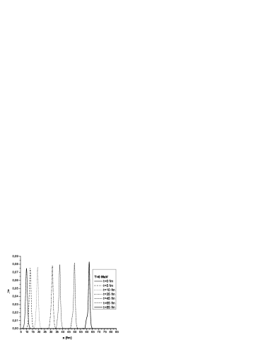
Figure 2: Time evolution of a baryon density pulse at zero temperature.

Fig. 3 shows the numerical solution of (30) for $A=0.35$ and $B=1$ fm. The time evolution of the pulse is similar to the one found in Fig. 2 but the “wall” formation and dispersion occurs much earlier.

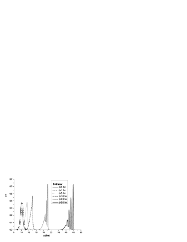
Figure 3: The same as Fig. 2 for a larger amplitude.

In Fig. 4 we present another solution of (30) for $A=0.075$ and $B=0.5$ fm.

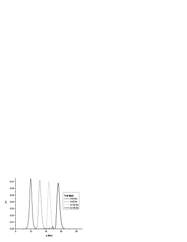
Figure 4: The same as Fig. 2 for a smaller width.

We can see that the initial pulse starts to develop small secondary peaks, which are called “radiation” in the literature. Further time evolution would increase the strenght of these peaks until the complete loss of localization.

From these figures we learn how the solution depends on the initial amplitude and width: it lives longer as a compact pulse for smaller amplitudes and larger widths. Changes in one quantity may compensate the changes in the other, creating a very stable moving object. In fact, the most striking conclusion to be drawn here is that for a wide variety of choices in the initial conditions the solution remains stable and localized for distances much larger than the nuclear size.

VI.2 Finite temperature

We now turn to the study of the solutions of (48) for initial conditions given by (52) (replacing $\hat{\rho}_{1}$ by $\hat{\varepsilon}_{1}$). Now, beside the amplitude and width, the solution will depend also on the temperature. When $T_{0}=T_{c}$ (48) reduces to:

$${\frac{\partial\hat{\varepsilon}_{1}}{\partial t}}+c_{S}{\frac{\partial\hat{\varepsilon}_{1}}{\partial x}}+{\frac{2}{3}}{c_{S}}\hat{\varepsilon}_{1}{\frac{\partial\hat{\varepsilon}_{1}}{\partial x}}=0$$ (53)

which, changing the function from $\hat{\varepsilon}_{1}$ to $\hat{\rho}_{1}$ is equal to (30). The previous conclusions are then extended to the present case. When $T_{0}>>T_{c}$ (48) reduces to:

$${\frac{\partial\hat{\varepsilon}_{1}}{\partial t}}+c_{S}{\frac{\partial\hat{\varepsilon}_{1}}{\partial x}}+{\frac{c_{S}}{2}}\hat{\varepsilon}_{1}{\frac{\partial\hat{\varepsilon}_{1}}{\partial x}}=0$$ (54)

Observing these two formulas we can see that, since $c_{s}=1/3$ is fixed, the only change in the differential equation with temperature happens in the numerical coefficient of the last term which goes from $0.5$ to $0.66$. Therefore our results depend very weakly on the temperature. A stronger dependence on $T$ would appear if $c_{s}$ was allowed to change with temperature. This would correspond to having a different and more complicated equation of state for the quark gluon plasma.

In Fig. 5 we show the solution of (48) with the initial condition given by (52) with $A=0.01$, $B=1$ fm and $T=300$ MeV.

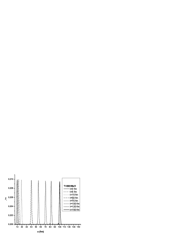
Figure 5: Time evolution of an energy density pulse at $T=300$ MeV.

Fig. 6 shows the same as Fig. 5 but with $A=0.1$ and $B=1$ fm. As in the zero temperature case, we observe that increasing the initial amplitude the breaking process develops earlier.

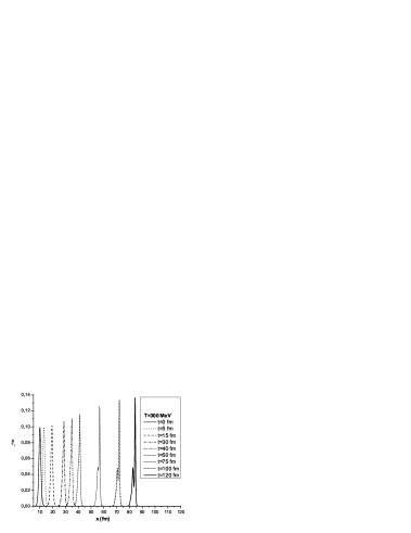
Figure 6: The same as Fig. 5 for a larger amplitude.

In Fig. 7 we show the same as Fig. 5 but with $A=0.01$ and $B=0.2$ fm. Figs. 8 and 9 show the time evolution of a pulse with the same initial amplitude ($A=0.5$) and width ($B=1$ fm) but different temperatures. Even though one temperature is $T=150$ MeV (Fig. 8) and the other is $T=300$ MeV (Fig. 9) we can hardly notice any difference.

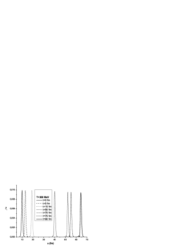
Figure 7: The same as Fig. 5 for a smaller width.

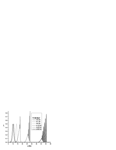
Figure 8: Evolution of the energy density pulse at $T=150$ MeV.

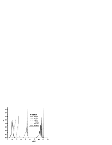
Figure 9: The same as Fig. 8 for $T=300$ MeV.

VII Conclusions

We have proposed an alternative explanation for the observed broadening of the away-side peak. It is based on the hydrodynamical treatment of energy perturbations. In contrast to other approaches we went beyond linearization of the fundamental equations and did not neglect the non-linear terms. We used a simple equation of state for the QGP and expanded the hydrodynamic equations around equilibrium configurations. The resulting differential equations describe the propagation of perturbations in the energy density. We solved them numerically and found that localized perturbations can propagate for long distances in the plasma. Under certain conditions our solutions mimick the propagation of Korteweg - de Vries solitons. However, as said before, from this finding to a realistic calculation and a serious attempt to describe the data there is still a long way. The main result found in this work, namely, the persistence of soliton-like configurations, is very promising and encourages us to extend our formalism to two spatial dimensions. This project is in progress.

- (1) J. Adams et al., STAR Collab. Phys. Rev. Lett. 95, 152301 (2005).
- (2) S. S. Adler et al. [PHENIX Collaboration], Phys. Rev. Lett. 97, 052301 (2006).
- (3) H. Stoecker, Nucl. Phys. A 750, 121 (2005); T. Renk and J. Ruppert, Phys. Rev. C 73, 011901 (2006) and references therein.
- (4) J. Casalderrey-Solana, E. Shuryak, E.V. and D. Teaney, J. Phys. Conf. Ser. 27, 22 (2005); Nucl. Phys. A 774, 577 (2006).
- (5) J. Ruppert and B. Muller, Phys. Lett. B 618, 123 (2005).
- (6) A. Chaudhuri and U. Heinz, Phys. Rev. Lett. 97, 062301 (2006).
- (7) T. Renk and J. Ruppert, Phys. Rev. C 73, 011901(R) (2006); Phys. Rev. C 76,014908 (2007); Phys. Lett. B 646, 19 (2007).
- (8) L. M. Satarov, H. Stoecker and I. N. Mishustin, Phys. Lett. B 627, 64 (2005); B. Betz, P. Rau and H. Stoecker, Int. J. Mod. Phys. E 16, 3082 (2008).
- (9) H. Stoecker, B. Betz and P. Rau, PoS C POD2006, 029 (2006); [arXiv:nucl-th/0703054].
- (10) R. B. Neufeld, B. Muller and J. Ruppert, Phys. Rev. C 78, 041901 (2008).
- (11) P.M. Chesler, L.G. Yaffe, hep-th/07060368; hep-th/07120050.
- (12) B. Betz, J. Noronha, G. Torrieri, M. Gyulassy and D. H. Rischke, arXiv:0907.2516 [nucl-th].
- (13) B. Betz, J. Noronha, G. Torrieri, M. Gyulassy, I. Mishustin and D. H. Rischke, Phys. Rev. C 79, 034902 (2009).
- (14) J. Noronha, M. Gyulassy and G. Torrieri, J. Phys. G 35, 104061 (2008).
- (15) B. I. Abelev et al. [STAR Collaboration], Phys. Rev. Lett. 102, 052302 (2009).
- (16) F. O. Durães, F. S. Navarra and G. Wilk, Phys. Rev. D 47, 3049 (1993).
- (17) D.A. Fogaça and F.S. Navarra, Phys. Lett. B 639, 629 (2006).
- (18) D.A. Fogaça and F.S. Navarra, Phys. Lett. B 645, 408 (2007).
- (19) D.A. Fogaça and F.S. Navarra, Nucl. Phys. A 790, 619c (2007); Int. J. Mod. Phys. E 16, 3019 (2007).
- (20) D.A. Fogaça, L. G. Ferreira Filho and F.S. Navarra, Nucl. Phys. A 819, 150 (2009).
- (21) S. Raha, K. Wehrberger and R.M. Weiner, Nucl. Phys. A 433, 427 (1984).
- (22) J.Y. Ollitrault, Eur. J. Phys. 29, 275 (2008).
- (23) R. C. Davidson, “Methods in Nonlinear Plasma Theory”, Academic Press, New York an London, 1972, pages 20 and 21.
- (24) G.N. Fowler, S. Raha, N. Stelte and R.M. Weiner, Phys. Lett. B 115, 286 (1982); S. Raha and R.M. Weiner, Phys. Rev. Lett. 50, 407 (1983); E.F. Hefter, S. Raha and R.M. Weiner, Phys. Rev. C 32, 2201 (1985).
- (25) A.Y. Abul-Magd, I. El-Taher and F.M. Khaliel, Phys. Rev. C 45, 448 (1992).
- (26) S. Weinberg,“Gravitation and Cosmology”, New York: Wiley, 1972.
- (27) L. Landau and E. Lifchitz, “Fluid Mechanics”, Pergamon Press, Oxford, (1987).
- (28) R. Reif, “Fundamentals os statistical and thermal physics”, New York: McGraw-Hill, 1965.
- (29) P. G. Drazin and R. S. Johnson, “Solitons: An Introduction”, Cambridge University Press, 1989.