Abstract:

Rapid energy releases (RERs) in the solar corona extend over many orders of magnitude, the largest (flares) releasing an energy of $10^{25}\;$J or more. Other events, with a typical energy that is a billion times less, are called nanoflares. A basic difference between flares and nanoflares is that flares need a larger magnetic field and thus occur only in active regions, while nanoflares can appear everywhere. The origin of such RERs is usually attributed to magnetic reconnection that takes place at altitudes just above the transition region. Here we show that nanoflares and smaller similar RERs can be explained within the drift wave theory as a natural stage in the kinetic growth of the drift wave. In this scenario, a growing mode with a sufficiently large amplitude leads to stochastic heating that can provide an energy release of over $10^{16}\;$J.

PACS numbers: 96.60.P-; 96.60.qe; 52.35.Kt

I.     INTRODUCTION

The central problems regarding rapid energy releases (RERs) are explaining i) where the energy comes from, ii) by what mechanism it is released, and iii) how it is transformed into (random and directed) particle energy. A widely (but not universally) used concept in the explanation of flares and other RERs, is that of magnetic reconnection which implies the presence of electric currents. Yet, the origin, and consequently the source of these currents, remains not well understood. Most frequently, shearing photospheric motions and/or magnetic flux emergence are used [1] in the models. The concept has been questioned in the past [2, 3] because of lack of a measurable magnetic energy and configuration change in some events [2, 4].

The electric field associated with RER events has been studied extensively in the past [5, 6, 7, 8], with very strong field reported [5] of $7\cdot 10^{4}\;$V/m , that may go [6] up to $1.3\cdot 10^{5}\;$V/m. As a rule, its presence is associated with the acceleration of lighter particles. Apart from the particle acceleration, flares and other smaller energy release events are responsible for strong local heating [9]. However, within the current models, it is nontrivial to explain how the released energy is dissipated so fast in the highly conductive corona, characterized by a Lundquist number around $10^{13}$. The existing continuum approximation (fluid) or magnetohydrodynamics (MHD) models, are not very promising because it is clear that the actual heating takes place at length scales much smaller than those on which the (macroscopic) MHD model is justified. We stress also that the possibility can not be excluded that, at least in some cases, the reconnection can appear as a consequence, rather than a cause of a RER. Another problematic aspect regarding the role of RERs in the heating, is the distribution of magnetic null points. According to Ref. [10] only 2% of them are located in the corona and 54% in the photosphere. This is opposite to what would be required for the mechanism that is presently believed to heat the corona. The heating by waves rather than by reconnection is also supported by the diagnostic of active regions presented in Ref. [11].

Here we present an alternative model of RERs and the consequent plasma heating, based on the kinetic theory of drift waves, driven by density gradients that are omnipresent in the solar corona. The model is able to provide answers to all the fundamental questions raised above. The required density gradients are visible in the magnetic loops spread throughout the solar atmosphere. They are closely connected to the continuous restructuring of the magnetic field (due to the frozen-in conditions), and also to the observed inflow of the plasma along the magnetic loops [12]. Measurements by Voyager 1 and Voyager 2 show [13, 14] that the transverse size of some of these highly elongated structures at the Sun can be below 1 km. Hinode observations [15] only confirm that the solar atmosphere is a highly structured and inhomogeneous system. Moreover, a three-dimensional analysis [16] of the coronal loops reveals short-scale density irregularities within each loop separately. Presently, the observable characteristic dimensions of density irregularities are limited by the available resolution of the instruments (at best about $0.5\;$arcsecond). However, even extremely short, meter-size scales can not be excluded. This can be seen by calculating the perpendicular (to the magnetic field) diffusion coefficient for a corona environment $D_{\bot,j}\approx\kappa T_{j}\nu_{j}/(m_{j}\Omega_{j}^{2})\propto m_{j}^{1/2}$, $j=i,e$. The diffusion velocity in the direction of the given density gradient is [17] $D_{\bot,j}\nabla n_{0}/n_{0}$. Taking the inhomogeneity scale-length $L_{n}\equiv[(dn_{0}/dx)/n_{0}]^{-1}=10,\,10^{2},\,10^{5}\;$m, where $x$-denotes the direction perpendicular to the magnetic field vector, we obtain the ion diffusion velocities, respectively, $10^{-3},10^{-4},10^{-7}\;$m/s only. Therefore, even very short density inhomogeneities can last long enough to support relatively high frequency drift instabilities. In dealing with the drift wave, we may thus operate with the density inhomogeneity scale lengths that can have any value from meter size up to thousands of kilometers in the case of coronal plumes. The role of the drift wave in RERs has been overlooked so far in the literature, probably due to the fact that it simply does not exist in the widely used MHD model.

The purpose of this work is to show that the free energy stored in these density gradients may drive drift waves, and these may further release energy on a massive scale. The dissipation of the drift waves is easy to explain in our self-consistent kinetic model that works on the (very small) length scales at which the actual dissipation takes place. Actually, two mechanisms of energy exchange and heating will be shown to take place simultaneously, one due to the Landau effect and another one, stochastic heating which acts exclusively in the perpendicular direction. To prove this we use only established basic theory, verified experimentally in laboratory plasmas.

II.     MODEL AND RESULTS

The drift wave properties within well known limits are described [18] by the frequency and the growth rate, respectively

$$\omega_{r}=-\frac{\omega_{*i}\Lambda_{0}(b_{i})}{1-\Lambda_{0}(b_{i})+T_{i}/T_{e}+k_{y}^{2}\lambda_{di}^{2}},$$ (1)

$$\gamma\simeq\left(\frac{\pi}{2}\right)^{1/2}\frac{\omega_{r}^{2}}{\omega_{*i}\Lambda_{0}(b_{i})}\left[\frac{T_{i}}{T_{e}}\frac{\omega_{r}-\omega_{*e}}{|k_{z}|v_{{\scriptscriptstyle T}e}}\exp[-\omega_{r}^{2}/(k_{z}^{2}v_{{\scriptscriptstyle T}e}^{2})]\right.$$

$$\left.+\frac{\omega_{r}-\omega_{*i}}{|k_{z}|v_{{\scriptscriptstyle T}i}}\exp[-\omega_{r}^{2}/(k_{z}^{2}v_{{\scriptscriptstyle T}i}^{2})]\right].$$ (2)

Here, $\Lambda_{0}(b_{i})=I_{0}(b_{i})\exp(-b_{i})$, $b_{i}=k_{y}^{2}\rho_{i}^{2}$, $\rho_{i}=v_{{\scriptscriptstyle T}i}/\Omega_{i}$, $\lambda_{di}=v_{{\scriptscriptstyle T}i}/\omega_{pi}$, $\omega_{*i}=-\omega_{*e}T_{i}/T_{e}$, $\omega_{*e}=k_{y}v_{*e}$, $\vec{v}_{*e}=-(v_{{\scriptscriptstyle T}e}^{2}/\Omega_{e})\vec{e}_{z}\times\nabla_{\perp}n_{0}/n_{0}$, $I_{0}$ is the modified Bessel function of the first kind and of the order 0, $\vec{B}_{0}=B_{0}\vec{e}_{z}$, and $\nabla_{\bot}=\vec{e}_{x}d/dx$.

In Eq. (2) the positive second term in the square bracket describes the damping on ions. The necessary condition for the instability $\omega_{r}<\omega_{*e}$, from the first term is, as a rule, easily satisfied. Note that Eq. (1) reveals the presence of the energy source already in the real part of the frequency $\omega_{r}\propto\nabla_{\bot}n_{0}$, while details of its growth due to the same source are described by Eq. (2).

In Fig. 1 we give the wave growth-rate as a function of two parameters, the perpendicular wavelength and the density scale-length $L_{n}$. The chosen parameters correspond to the inner corona, i.e., $B_{0}=5\cdot 10^{-3}\;$T, $n_{0}=10^{16}\;$m^-3, $T_{i}=T_{e}=T_{0}=7\cdot 10^{5}\;$K. The graph does not change drastically by varying these parameters for $\pm 1$ order of magnitude. The wavelength parallel to the magnetic field vector is taken as $\lambda_{z}=s\cdot 10^{4}\;$m. We have introduced a parameter $s$ that we can vary within the range $10^{-1}-10^{3}$ in order to demonstrate that the mode behavior remains unchanged at various density scale lengths $L_{n}$, provided that we keep the ratio $\lambda_{z}/L_{n}$ constant. It can easily be shown that in this case the ratio $\gamma/\omega_{r}$ also remains constant [19, 20], while both quantities are shifted either to lower or higher values. As example, the mode frequency for $s=1$, $L_{n}=100\;$m, and $\lambda_{y}=1\;$m is $\omega_{r}=231\;$Hz, and it changes as $231/s$ when the other parameters are fixed. The growth rate may easily become larger than $\omega_{r}$ for short $\lambda_{y},L_{n}$.

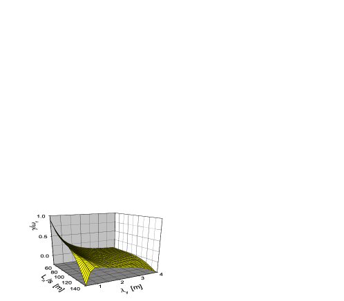
Figure 1: The growth rate (2) normalized to the wave frequency $\omega_{r}$ in terms of the perpendicular wavelength and the density scale-length $L_{n}$.

The growth of the wave results in a stochastic heating mechanism that implies single particle interaction with the wave. The process has been experimentally verified [21, 22]. In the drift wave, the ions move in the perpendicular direction to large distances and they feel the time-varying field of the wave due to the polarization drift $\vec{v}_{p}=(d\vec{E}/dt)/(\Omega_{i}B_{0})$, and as a result their motion becomes stochastic. This stochastic heating is anisotropic, acting mainly in the direction normal to the magnetic field $B_{0}$. The perpendicular heating in the experiment was larger by about a factor 3 compared to the parallel one [21, 22], and it is exceptionally fast. It the same time, in view of the mass difference and the given physical picture, this heating scenario predominantly acts on the ions, with heavier ions more efficiently heated than lighter ones. For drift wave electrostatic potential perturbation of the form $\phi(x)\sin(k_{y}y+k_{z}z-\omega t)$, $|k_{y}|\gg|k_{z}|$, one finds the ion polarization drift velocity following the procedure from Ref. [23]. For large enough particle displacements (large wave amplitudes) $\vec{v}_{p}=\vec{e}_{y}[k_{y}\phi/(\Omega_{i}B_{0})](d/dt)\sin(k_{y}y-\omega t)=\vec{e}_{y}[k_{y}\phi/(\Omega_{i}B_{0})](k_{y}dy/dt-\omega)\cos(k_{y}y-\omega t)$, where $dy/dt=v_{p}$. This yields

$$\vec{v}_{p}=-\vec{e}_{y}\frac{\omega k_{y}\phi}{\Omega_{i}B_{0}}\frac{\cos(k_{y}y-\omega t)}{1-a\cos(k_{y}y-\omega t)},$$ (3)

$$a=k_{y}^{2}\rho_{i}^{2}e\phi/(\kappa T_{i}).$$

It has been shown [22] that the stochastic heating takes place for a large enough wave amplitude, more precisely for $a\geq 1$. This condition implies that the ion displacement due to the polarization drift is comparable to the perpendicular wavelength. This is because $\vec{v}_{p}=(\vec{e}_{z}\times\partial\vec{v}_{\bot}/\partial t)/\Omega_{i}$, and $\vec{v}_{\bot}$ is the leading order $\vec{E}\times\vec{B}$-drift, so that $v_{p}\sim a\omega/k_{y}$ and the perpendicular displacement due to the polarization drift is $\delta=v_{p}/\omega=a/k_{y}$. Another important feature is that $\vec{v}_{p}\sim\vec{k}_{y}$, hence the stochastic heating is due to the electrostatic property of the wave.

According to [21, 22], the maximum achieved bulk ion velocity, proportional to the wave amplitude, is given by

$$v_{m}\simeq[k_{y}^{2}\rho_{i}^{2}e\phi/(\kappa T_{i})+1.9]\Omega_{i}/k_{y}.$$ (4)

As explained in Ref. [22], the factor $1.9$ appears after making Pincaré plots of particle trajectories for different values of $a$. Slightly different values of this factor, i.e., 1.5 and 2.3, are reported in Refs. [24, 25], respectively.

Eq. (4) implies an effective increase in the temperature $T_{ef}=m_{i}v_{m}^{2}/(3\kappa)$, while the volumetric energy increase of the stochastically heated particles is $\Sigma_{m}=n_{0}m_{i}v_{m}^{2}\;$ [J/m³], and the energy release rate is $\Gamma_{m}=\Sigma_{m}/\tau_{g}\;$ [J/(m³s)], where $\tau_{g}=1/\gamma$.

Equation (4) reveals a minimum of $v_{m}$ at $\lambda_{y}=2\pi\rho_{i}[e\phi/(\kappa T_{i})]^{1/2}$. This is seen also in Fig. 2. Here, we fix $\phi=10^{3}\;$V and use the same parameters as in Fig. 1.

Figure 2: Volumetric energy released during stochastic heating by the drift wave in terms of the perpendicular wavelength.

Since the results are valid for any $s$, the growth time $\tau_{g}\propto s$ may have rather different values. Assuming a small accidental initial perturbation $e\phi_{0}/(\kappa T_{i})=0.01$ the growth time till it gets the value used above is $\tau_{g}=\log(\phi/\phi_{0})/\gamma$. Taking $s=1$ and $s=10^{3}$, at the minimum from Fig. 2 we obtain $\tau_{g}\simeq 0.2\;$s, and $\tau_{g}\simeq 3.3\;$min, respectively. The same dependence on $s$ holds for the total plasma volume $V_{p}=L_{x}L_{y}L_{z}$ involved in RERs, and consequently for the total amount of the released energy. We may take $L_{x}=L_{n}$, and for $L_{z}$ take one wavelength $\lambda_{z}$ only while for $L_{y}$ we may take a layer of around $10\;$km. At the minimum $\lambda_{y}$ from Fig. 2 and for $s=10^{3}$, this yields $\Sigma_{m}V_{p}=1.5\cdot 10^{16}\;$J. Clearly, this value can easily become considerably larger (e.g., for a larger volume, then for $\lambda_{y}$ not taken at minimum, and also increasing the density for one order of magnitude will increase the energy for one order too).

Calculating $dT_{ef}(m_{i})/dm_{i}$ it can be shown that the heating increases with ion mass if $k_{y}^{4}\rho_{i}^{4}[e\phi/(\kappa T_{i})]>1.9$. For the parameters of interest here, it turns out that this condition is always satisfied. We stress that numerous indications and observations in the solar corona [26, 27, 28] confirm these peculiar features of a stronger heating of heavier particles, i.e., $T_{e}<T_{H}<T_{He}$, and a stronger heating in the perpendicular direction as compared to the heating along the magnetic field vector.

The drift mode presented above implies a time-varying electric field. Its parallel component $|\nabla_{z}\phi|$ for $\lambda_{z}=s\cdot 10\;$km (in units of the Dreicer runaway electric field) is $4$ and $0.004$ for $s=1$ and $10^{3}$, respectively. In the first case, the bulk plasma species (primarily electrons) can be accelerated by the wave in the $z$-direction. In the latter, this holds only for electrons from the tail in the distribution function. Hence, in any case there will be an increase in the directed electron energy. The escaping electrons imply that a smaller amount of them are available to shield ion perturbations and the mode should be even more growing. The electron parallel velocity in a time-varying parallel wave-electric field $E_{0}\cos(k_{z}z-\omega_{r}t)$ is

$$v(t)=v_{0}-\frac{eE_{z}}{m_{e}(k_{z}v_{0}-\omega_{r})}\left\{\sin[k_{z}z_{0}+(k_{z}v_{0}-\omega_{r})t]\right.$$

$$\left.-\sin(k_{z}z_{0})\right\}.$$ (5)

Here $v_{0}$ and $z_{0}$ are the starting electron velocity and position in the parallel direction, respectively. A strong acceleration will take place, in particular for particles close to resonance $v_{0}=\omega_{r}/k_{z}=0.1v_{{\scriptscriptstyle T}e}$. The non-relativistic energy radiated by an electron decelerated in the time-varying wave electric field is given by $\Delta\Sigma/\Delta t=e^{2}(\Delta v/\Delta t)^{2}/(6\pi\varepsilon_{0}c^{3})$. Here, $\Delta t\simeq\tau_{osc}/4$, where $\tau_{osc}=2\pi/(k_{z}v_{0}-\omega_{r})$. It is seen that for particles close to resonance, the oscillation period $\tau_{osc}$ becomes very large and the same holds for the particle velocity. So the previously described process of stochastic heating will be accompanied by a large directed acceleration and by radiation as well.

For plasma $\beta$ above the electron/ion mass ratio the drift wave couples with the Alfvén wave. This coupling is given by [29, 30] $\omega^{3}-\omega^{2}(\omega_{*e}+\omega_{*i})+\omega[\omega_{*e}\omega_{*i}-k_{z}^{2}c_{a}^{2}/(1+k_{y}^{2}\rho_{i}^{2})-k_{y}^{2}k_{z}^{2}c_{a}^{2}(\rho_{i}^{2}+\rho_{s}^{2})]+k_{z}^{2}c_{a}^{2}\omega_{*e}/(1+k_{y}^{2}\rho_{i}^{2})=0$, $c_{a}^{2}=B_{0}^{2}/(\mu_{0}n_{0}m_{i})$. It describes the drift wave and two Alfvén waves. The electromagnetic effects in RERs are frequently (but not always) observed. However, even in the presence of coupling, the previous analysis related to the energy release will not change considerably. This can be checked by solving the above dispersion equation for the coupled modes and comparing to previous results. As example, for $\lambda_{y}=3$ m, $s=10^{3}$ and other parameters unchanged, the drift wave frequency from Eq. (1) is $0.21$ Hz, while from the coupled mode it is $0.25$ Hz.

III.     SUMMARY

The model and results presented here, based on the drift wave theory, yield an alternative description of some rapid energy releases in the solar corona. Because of a high temperature and a low number density, collisions are rare in coronal magnetic structures, hence the kinetic description of the drift wave is the most appropriate. In such a description the drift wave is strongly growing and its growth-rate appears as a purely kinetic effect.

Using parameters typical for inner corona we have shown that such a growing drift wave can lead to stochastic heating of ions,²⁰ with the heating rate so large that can be used for the description of nano-flares and smaller energy releases. We have also shown that there should be an acceleration of plasma particles, primarily electrons, by growing drift waves in solar corona. Such an acceleration and heating of coronal plasma has been discussed in many studies in the literature in the past,^31-33 yet not within the drift wave theory. Our analysis comprises the electrostatic limit, which may be appropriate at least in some cases because observations in the past have shown that not all rapid energy releases are associated with a measurable change in the magnetic field topology. However, using the well known theory the magnetic effects can be included and they would lead to the coupling between the drift and Alfvén waves, and this limit is also briefly discussed.

The model implies the density gradients in the background plasma, that are expected within coronal magnetic structures. Since the growth of the mode is on the account of the energy stored in this gradient, it is expected that the background is simultaneously changed in the process of the instability. Simulation in the past have shown this.³⁴ As a result the energy release should be below the value obtained in the present study. A detailed description of this feedback effect can be performed only numerically, yet this is beyond the scope of the present work.

References

- [1] M. S. Wheatland, Astrophys. J. 679, 1621 (2008).
- [2] T. J. Janssens, Solar Phys. 27, 149 (1972).
- [3] M. I. Pudovkin, S. A. Zaitseva, N. O. Shumilov, and C. V. Meister, Solar Phys. 178, 125 (1998).
- [4] E. B. Mayfield and G. A. Chapman, Solar Phys. 70, 351 (1981).
- [5] W. D. Davis, Solar Phys. 54, 139 (1977).
- [6] Z. Zhang and R. N. Smartt, Solar Phys. 105, 355 (1986).
- [7] A. O. Benz, Solar Phys. 111, 1 (1987).
- [8] P. Foukal and S. Hinata, Solar Phys. 132, 307 (1991).
- [9] M. J. Aschwanden, Physics of the Solar Corona (Springer-Verlag, Belin-Heidelberg-New York, 2004), p. 387.
- [10] S. Régnier, C. E. Parnell, and A. L. Haynes, Astron. Astrophys. 484, L47 (2008).
- [11] R. O. Milligan, P. T. Gallagher, M. Mathioudakis, F. P. Keenan, and D. S. Bloomfield, Month. Not. Roy. Astron. Soc. 363, 259 (2005).
- [12] C. J. Schrijver et al., Solar Phys. 187, 261 (1999).
- [13] R. Woo and S. R. Habbal, Astrophys. J. 474, L139 (1997).
- [14] R. Woo, Nature 379, 321 (1996).
- [15] B. De Pontieu et al., Science 318, 1574 (2007).
- [16] M. J. Aschwanden, J. P. Wülser, N. V. Nitta, and R. R. Lemen, Astrophys. J. 679, 827 (2008).
- [17] J. Vranjes and S. Poedts, Astron. Astrophys. 482, 653 (2008).
- [18] S. Ichimaru, Basic Principles of Plasma Physics (The Benjamin/Cummings Publish. Comp., Reading, Massachusetts, 1980).
- [19] J. Vranjes and S. Poedts, Month. Not. Roy. Astron. Soc., to be published (2009).
- [20] J. Vranjes and S. Poedts, EPL 86, 39001 (2009).
- [21] J. M. McChesney, R. A. Stern, and P. M. Bellan, Phys. Rev. Lett. 59, 1436 (1987).
- [22] S. J. Sanders, P. M. Bellan, and R. A. Stern, Phys. Plasmas 5, 716 (1998).
- [23] P. M. Bellan, Fundamentals of Plasma Physics (Cambridge Univ. Press, Cambridge, UK, 2006), p. 106.
- [24] J. F. Drake and T. T. Lee, Phys. Fluids 24, 1115 (1981).
- [25] J. M. McChesney, P. M. Bellan, and R. A. Stern, Phys. Fluids B 3, 3370 (1991).
- [26] V. N. Hansteen, E. Leer, and T. E. Holtzer, Astrophys. J. 482, 498 (1997).
- [27] I. Cuseri, D. Mullan, and G. Poletto, G., Space Sci. Rev. 87, 153 (1999)
- [28] S. R. Cranmer, A. V. Panasyuk, and J. L. Kohl, Astrophys. J. 678, 1480 (2008).
- [29] J. Vranjes and S. Poedts, Astron. Astrophys. 458, 635 (2006).
- [30] J. Weiland, Collective Modes in Inhomogeneous Plasmas (Institute of Physics Pub., Bristol, 2000).
- [31] S. Saito and Y. Sakai, Phys. Plasmas 11, 5547 (2004).
- [32] R. Jain, P. Browning, and K. Kusano, Phys. Plasmas 12, 012904 (2005).
- [33] I. H. Cairns and B. F. McMillan, Phys. Plasmas 12, 102110 (2005).
- [34] D. Tsiklauri, Phys. Plasmas 15, 112903 (2009).