The scale of market quakes

Abstract

We define a methodology to quantify market activity on a 24 hour basis by defining a scale, the so-called scale of market quakes (SMQ). The SMQ is designed within a framework where we analyse the dynamics of excess price moves from one directional change of price to the next. We use the SMQ to quantify the FX market and evaluate the performance of the proposed methodology at major news announcements. The evolution of SMQ magnitudes from 2003 to 2009 is analysed across major currency pairs.

PACS: 89.65.Gh, 89.75.Da, 89.75.Fb.

JEL: C53, D40, E32, E37, G01.

Keywords: Financial Markets; Currency markets; Market Activity; Market Impact; High Frequency Data; Market Microstructure; Scaling Laws; Volatility; Financial Crisis

1 Introduction

Prices in financial markets evolve as events occur. Events are typically market transactions, which may be correlated with each other, or news and political announcements. The price evolution occurs in many different forms and is difficult to describe concisely as price moves happen at all different price and time scales. For instance, a $1\%$ price move can occur within a few seconds and the price jumps to its new level, within a few minutes and the price is subject to a secondary counter price move or alternatively for a few days the price may zigzag within a narrow price range. These examples highlight the importance of creating a tool coming up with a concise abstraction that characterises the price evolution in a systematic manner so as to be a reliable representation of the state of the market at any point in time and after any type of market events. We believe that a proper tool to characterise market events is an essential element towards building a financial warning system [1].

The pioneering work of Zumbach et al. [2] has defined, for the currency market, the so-called scale of market shocks that quantifies market movements on a tick-by-tick basis as a weighted average of volatilities over different time horizons. In [2], the scale of market shocks is used to measure the impact of major events between 1998 and 1999 for a couple of exchange rates. This approach, certainly interesting, mainly suffers from being too complicated as too many ad-hoc choices of functions and fittings have been made. Also we note the arbitrary weighting of time horizons that can make the scale of market shocks to over- or in the contrary underweight a given time-scale, therefore distorting the measurement.

Maillet and Michel [3] have adapted the scale of market shocks to the stock market. The new indicator is designed for the detection and comparison of severity of different crises and suffers from the same deficiencies as its ancestor. It is also worth mentioning the unpublished work by Subbotin [4] which, also inspired by [2], has proposed a probabilistic indicator for volatilities by decomposing volatility of stock market indexes using wavelets. Wavelet decomposition is used to circumvent the mixing of scales in [2]. This latter indicator seems to be usable for detecting crisis or regime shifts rather than quantifying impact of single events as we observe periods up to a year over which the indicator has a significant value.

For the choice of a metric to measure market evolution there cannot be a right or wrong. There are, however, two criteria for such a metric that seem particularly important: simplicity and ability to incorporate all the details of the price evolution of the time series. We claim that the previous attempts presented above have not been able to maximise these criteria. Authors in [2, 3, 4] have chosen volatility of the market to characterise its state. Although this sounds like a natural choice, we argue that aggregating market activity into a volatility measurement is not the most appropriate as activity at different price scales are mingled. In addition, we stress that only the high frequency definition of volatility in [2] prevents information to be lost through homogenising the time series, and even more important every time increment has the same weight.

Inspired by the discovery of a large number of scaling laws [5], we propose a framework in which price directional changes set the rhythm and where we monitor the excess price moves from one directional change to the next, the so-called overshoot, at different price scales. Within this novel and simple framework, physical time does not exist anymore and is replaced by intrinsic time (ticking at every occurrence of a directional change of price). The average of price overshoots does not exhibit the drawbacks of volatility as representative price scales, and all active time scales, are taken into account. Within this framework, we design a methodology to quantify impact of multi-scale events along a scale, the so-called scale of market quakes (SMQ) which defines a tick-by-tick metric allowing us to quantify market evolution on a continuous basis. Without loss of generality, we apply our methodology to the FX market and publish real time magnitudes online at [6].

Related literature in the field explores how transactions impact the market (see [7] and references therein). In contrast, we are here interested to develop tools to quantify in an objective manner the trajectory of market prices evolution.

The document is organised as follows. We first describe the methodology defining the SMQ and show various news announcement snapshots to highlight the usefulness of the scale. We then analyse the evolution of magnitudes along the SMQ over the years across major currency pairs. Finally we conclude and discuss further work.

2 Methodology

2.1 An event discretisation of the price curve

It is custom to discretise the price curve along its temporal axis by computing the return $r$ as the price difference within a time interval $\Delta t$

$$r(t)=\log p(t)-\log p(t-\Delta t)$$ (1)

where $p(t)$ is the homogeneous, and therefore interpolated, sequence of prices. Volatility and other statistical analysis are computed from the time series (1).

Because market prices change at irregular time intervals, measurement of market activity in terms of discrete $\Delta t$ needs to be adaptive. To achieve that we propose an event based approach that considers the sequence of price directional changes of magnitude $\lambda$[5, 8]. Within that framework time passes by unevenly: any occurrence of a directional change represents a new intrinsic time unit.

A directional change of magnitude $\lambda$ is usually not immediately followed by an opposite directional change but rather by a price overshoot $\omega(t,\lambda)$ where $t$ denotes time. The price overshoot is of particular interest as it measures the excess price move along a $\lambda$ scale and can be used as a market activity quantifier. Figure 1 shows how the price curve is dissected into directional change and overshoot sections.

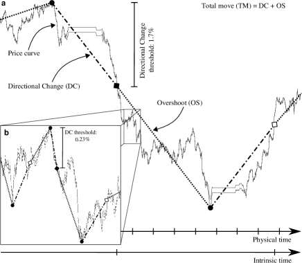
Figure 1: Projection of a (a) two-week, (b) zoomed-in 36 hour price sample onto a reduced set of so-called directional change events defined by a threshold (a) $\lambda=1.7\%$, (b) $\lambda=0.23\%$. These directional change events (diamonds) act as natural dissection points, decomposing a total price move between two extremal price levels (bullets) into so-called directional change (solid lines) and overshoot (dashed lines) sections. Time scales depict physical time ticking evenly across different price curve activity regimes, whereas intrinsic time triggers only at directional change events.

The dynamics of overshoots organises as follows. Every occurrence of a directional change triggers a new overshoot which will swing between $-\lambda$ and any positive value until it decreases by $-\lambda$ making the next directional change to occur. Figure 2(a) shows the overshoot dynamics.

(a)
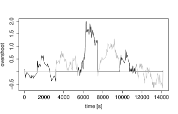
(b)

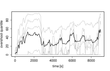
Figure 2: Sample evolution of (a) the price overshoot $\omega(t)$ and (b) the average price overshoot $\bar{\omega}(t)$. (a) Alternated gray and black lines show the overshoot normalised by $\lambda$. (b) A subset of the $n_{\lambda}$ thresholds are shown in gray and the black line shows the average overshoot $\bar{\omega}(t)$. Overshoots are measured in quantiles to ensure a normalised measurement.

In order to capture the market activity, that is not occurring at a single price scale, we define an average overshoot $\bar{\omega}$ as

$$\bar{\omega}(t)=\frac{1}{n_{\lambda}}\sum_{i=1}^{n_{\lambda}}\omega^{q}(t,\lambda_{i})$$ (2)

where $n_{\lambda}$ is the number of thresholds $\lambda_{i}$ and the superscript $q$ on $\omega^{q}(t)$ denotes the fact that the overshoot $\omega(t)$ is here expressed in quantiles where the tick-by-tick historical distribution of price overshoots from December 1, 2005 up to December 31, 2008 is considered. Overshoots are normalised by using quantiles so as to be averaged over different thresholds. We consider evenly distributed thresholds and set $\lambda_{i}=i\cdot 0.05\%$ with $i$ running from $1$ to $n_{\lambda}=100$. It is worth to note at this stage that both $\omega(t)$ and $\bar{\omega}(t)$ are inhomogeneous. Figure 2(b) shows the time evolution of $\bar{\omega}$.

2.2 The scale of market quakes

We now describe the way the average overshoot $\bar{\omega}(t)$ is converted into a unique number $\mathcal{S}(t)$ along the scale of market quakes. It is defined as

$$\mathcal{S}(t)=\frac{1}{n_{a}}\sum_{i=0}^{n_{a}}\mathcal{F}(\Omega(t+(\frac{i}{n_{a}}-0.5)\delta t))$$ (3)

where $\delta t=2$ hours is the time window, $n_{a}=\delta t/\delta t_{a}$ with $\delta t_{a}=15$ minutes and the set $\Omega(t)=\{\bar{\omega}(\tau)-\left<\bar{\omega}(\tau)\right>\;|\;t-\delta t/2\leq\tau\leq t+\delta t/2\}$. The average operator $\left<\cdot\right>$ is taken over $[t-\delta t/2;t+\delta t/2]$ and is used to prevent high or low plateaux to correspond to significantly different frequencies. The operator $\mathcal{F}(\cdot)$ is defined as

$$\mathcal{F}(\Omega(t))=\frac{1}{n_{f}}\sum_{k=0}^{n_{f}-1}\frac{|X_{k}|}{k+1}$$ (4)

where $n_{f}=\delta t/\delta t_{f}$ is the number of discretisation points of $\Omega(t)$ and $|X_{k}|$ is the magnitude of the Fourier frequency computed from the discretised $\Omega(t)$. $\delta t_{f}=7$ seconds is chosen to be precise enough but computationally doable on a 24 hour basis, and so is set to be as near as possible to a power of 2 required for an efficient computation of the Fourier transform: $n_{f}=1028$ where the 4 first values are disregarded. As a discrete Fourier transform of a signal composed of real values obeys the symmetry $X_{k}=X_{n_{f}-k}$, we set $n_{f}=\lfloor n_{f}/2+1\rfloor$. Dividing the frequencies by $k+1$ ensures the robustness of the operator $\mathcal{F}(\cdot)$ to small perturbations.

The SMQ methodology is associated to a time lag of $\delta t=2$ hours as computing a magnitude along the SMQ at time $t$ requires to know the time series up to $t+\delta t/2$ for computing $\mathcal{F}(\Omega(t+\delta t/2))$ and to a further $\delta t/2$ for properly defining $\Omega$. To alleviate this issue we compute preliminary values by reducing the averaging scope $n_{a}$ of eq (3) and set $n_{a}=\{0,2,4,6\}$ providing estimates after 60, 75, 90, 105 minutes respectively. On average we note that estimates are roughly $20\%$ higher than final values, see [6].

We observe from (3) that magnitudes along the SMQ are strictly positive. An upper bound is found by manipulating the discrete Fourier transform definition to find a frequency bound, and then injecting it into (3). After some simple algebra one finds

$$\mathcal{S}(t)\leq 50\sum_{k=0}^{n_{f}-1}\frac{1}{k+1}.$$ (5)

However, as we shall see, $\mathcal{S}(t)$ is usually smaller than $10$ and eq (5) hardly reaches its limits as it corresponds to a theoretical case.

3 Results

We use the SMQ to analyse the market on a 24 hour basis and evaluate the performance of the proposed methodology at major news announcements in the FX market. Then we examine the evolution of SMQ magnitudes between January 2004 up to August 2009 and across different currency pairs. We stress here that the SMQ methodology is also applicable to other asset classes.

3.1 Quakes at event time

Figure 3(a-h) shows the behaviour of EUR-USD and the SMQ on the occasion of 8 releases of non-farm employment numbers [9]. The wide variety of market responses: a steep drop (f), the same price move amplitude as in (f) but happening within a longer time period (e), little reaction from the market (c), volatile market (g,h) or a drop immediately followed by a recovery (b,g) is characterised by our methodology computing a single number within the SMQ. As expected we observe that the steep drop (f) is associated to a higher value than (e) where the difference between the two scenarios is mainly the time for the price move to occur. Scenario (b), that could well go unnoticed as the original price level does not seem to be altered by the news announcement, is given a significant magnitude that is comparable to (e).

We also notice in figure 3(a,b,d) that peaks of magnitude do not always coincide with releasing time as the market response can take a few hours to operate.

It is also interesting to remark that similarly to earthquakes, after-quakes occur such as in (a,g), and have, in contrast to what is shown here, also been observed to be stronger than the original quake. A reason for this might be that the first market reaction could trigger further actions producing in turn market impacts of bigger magnitude.

Figure 3(i) shows the distribution of the magnitude of two sets of events versus the maximum price move that occurred within the next 12 hours following the events. The first events considered are 27 non-farm employment change announcements between 2007 and 2009, and the second ones are 4687 magnitude peaks observed between December 2005 and March 2009 where a magnitude peak corresponds to a value $\mathcal{S}(t)$ where $\mathcal{S}(t)>\mathcal{S}(t\pm 2\delta t_{a})$.

We observe a cone-like structure where large magnitudes do not correspond to any small price moves but where large price moves can be associated to small magnitudes. This is because a large magnitude necessarily implies that high price thresholds are activated but on the other hand a noticeable price move can happen as a jump in the market and therefore does not necessarily correspond to a large magnitude.

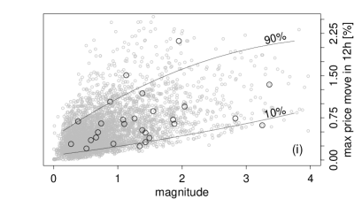
Figure 3: (a-h) Behaviour of EUR-USD (thin lines) and the SMQ (thick line). The announcement time is depicted by a dashed line and its date appears on the top left of the figure. (i) Distribution of the magnitude of two sets of events versus the maximum price move that occurred within the next 12 hours following the events. The first events (black circles) are 27 non-farm employment change announcements between 2007 and 2009, and the second ones (gray circles) are 4687 magnitude peaks observed between December 2005 and March 2009 where a magnitude peak $\mathcal{S}(t)$ is defined as $\mathcal{S}(t)>\mathcal{S}(t\pm 2\delta t_{a})$. The $10\%$ and $90\%$ quantiles of the distribution are shown.

For the sake of the presentation we have shown here only data related to EUR-USD and only considered US news. There are no obstacles towards considering other currency pairs and news and we are, as we write, applying this methodology to 24 currency pairs and publishing magnitudes related to the main international news at [6].

3.2 Time evolution of the magnitude

We now analyse the time evolution of SMQ magnitudes and define the magnitude likelihood $l_{n_{d}}(t,k)$ at time $t$ as the probability to observe a magnitude to be larger or equal than a threshold magnitude $k$, within the last $n_{d}$ days

$$l_{n_{d}}(t,k)=\frac{1}{n_{\rho}+1}\sum_{i=0}^{n_{\rho}}\mathcal{N}(t-i\;2\delta t_{a})$$ (6)

where $n_{\rho}=n_{d}/2\delta t_{a}$ is the number of computed magnitudes within the backward looking time window of $n_{d}$ days, and where $\mathcal{N}(t)=1$ if $\mathcal{S}(t)\geq k$ and $\mathcal{N}(t)=0$ otherwise. In the following analysis we arbitrarily set a medium-term time window of $n_{d}=100$ days.

Figure 4 shows the evolution of the magnitude likelihood $l_{100}(t,k)$ for representative currency pairs, between July 2003 to August 2009 where magnitude thresholds $k$ varies from 1 to 6. As expected from definition (6), we observe that the smaller the threshold $k$, the larger the likelihood as $l_{n_{d}}(t,k_{1})\leq l_{n_{d}}(t,k_{2})$ if $k_{1}\leq k_{2}$.

Overall, figure 4 shows decreasing likelihoods from July 2003 up to the middle of 2007. Then the first FX market response to the credit crisis shows: likelihoods exhibit bumps which peek at the highest amplitude so far and vanish in the middle of 2008. These peeks appear in the first quarter of 2008 implying that violent price moves that occurred in summer 2007 might be responsible for these local extrema. It then follows the second market response as we observe sharp likelihood increases at the end of 2008. This is followed by significant decreases over 2009 as we measure up to a factor 4 between the maximum magnitude and the latest one in August 2009. Figure 4 seems then to indicate that activity is calming down in 2009, without yet indicating anything on what could happen next. The forecasting ability of this approach is however of interest and will be subject to further communication.

Figure 4(b) depicts the dynamics of EUR-CHF that seems to behave in a somewhat different way as compared to other currency pairs presented in figure 4. Indeed, magnitude likelihoods appear to be smaller than $5\%$ for all magnitude thresholds, up to 2008. This is in line with a recent study by Glattfelder et al. [5] who present a new set of 17 scaling laws that behave in a different way within EUR-CHF than within any other of the 13 analysed currency pairs. The reason for that might be that the ratio between volatility and spread (difference between bid and ask) is lower in EUR-CHF than in any other currency pair analysed here making it less attractive to speculative traders, and therefore generating less activity.

(a) AUD-USD
(b) EUR-CHF
(c) EUR-JPY
(d) GBP-USD
(e) NZD-USD
(f) USD-CAD
(g) USD-CHF
(h) USD-JPY
(i) EUR-USD

Figure 4: Time evolution of magnitude likelihoods $l_{100}(t,k)$ from July 2003 to August 2009 across representative currency pairs. Nested curves related to different magnitude threshold $k\in[1;6]$ are shown.

The analysis of the evolution of likelihoods would be enhanced by considering the average of likelihoods expressed in quantiles over all thresholds. A large average value would indicate an increase of likelihood at all scales therefore highlighting the probable start of a turbulent phase. We however leave this point for a further study.

4 Conclusion

We have proposed a new and simple way of quantifying price behaviour by computing magnitudes of quakes along the scale of market quakes. The SMQ acts on a tick-by-tick basis [6] and quantifies multi-scale events occurring in the market in response to news announcements or a mismatch of demand and supply. The SMQ is a metric to measure the impact of these events.

We believe that the SMQ is a first step towards a global information system [1] that we urgently need in order to asses the state of the economy and its financial markets. The information system would allow economic agents, be they governments or private and institutional investors to take more informed decisions and adopt preemptive action in a crisis.

5 Acknowledgements

We thank J.B. Glattfelder for providing us with figure 1.

References

- [1] R.B. Olsen and C. Cookson. How science can prevent the next bubble. Financial Times, Feb 12 2009.
- [2] G.O. Zumbach, M.M. Dacorogna, J.L. Olsen, and R.B. Olsen. Measuring shock in financial markets. Int. J. Theoretical Appl., 3:347, 2000.
- [3] B. Maillet and T. Michel. An index of market shocks based on multiscale analysis. Quant. Finan., 3:88, 2003.
- [4] A. Subbotin. A multi-horizon scale for volatility. Available at http://hal-paris1.archives-ouvertes.fr/docs/00/26/15/14/PDF/Bla08020.pdf, 2008.
- [5] J.B. Glattfelder, A. Dupuis, and R.B. Olsen. An extensive set of scaling laws and the FX coastline. Quant. Financ., submitted. arXiv:0809.1040.
- [6] www.olsenscale.com.
- [7] J.-P. Bouchaud, J.D. Farmer, and F. Lillo. How markets slowly digest changes in supply and demand. In T. Hens and K. Schenk-Hoppe, editors, Handbook of Financial Markets: Dynamics and Evolution. Elsevier: Academic Press, 2008.
- [8] M. M. Dacorogna, R. Gençay, U. A. Müller, R. B. Olsen, and O. V. Pictet. An introduction to high-frequency finance. Academic Press, San Diego, San Diego, 2001.
- [9] Bureau of Labor Statistics. www.bls.gov.