The Carnegie Astrometric Planet Search Program

Abstract

We are undertaking an astrometric search for gas giant planets and brown dwarfs orbiting nearby low mass dwarf stars with the 2.5-m du Pont telescope at the Las Campanas Observatory in Chile. We have built two specialized astrometric cameras, the Carnegie Astrometric Planet Search Cameras (CAPSCam-S and CAPSCam-N), using two Teledyne Hawaii-2RG HyViSI arrays, with the cameras’ design having been optimized for high accuracy astrometry of M dwarf stars. We describe two independent CAPSCam data reduction approaches and present a detailed analysis of the observations to date of one of our target stars, NLTT 48256. Observations of NLTT 48256 taken since July 2007 with CAPSCam-S imply that astrometric accuracies of around 0.3 milliarcsec per hour are achievable, sufficient to detect a Jupiter-mass companion orbiting 1 AU from a late M dwarf 10 pc away with a signal-to-noise ratio of about 4. We plan to follow about 100 nearby (primarily within about 10 pc) low mass stars, principally late M, L, and T dwarfs, for 10 years or more, in order to detect very low mass companions with orbital periods long enough to permit the existence of habitable, Earth-like planets on shorter-period orbits. These stars are generally too faint and red to be included in ground-based Doppler planet surveys, which are often optimized for FGK dwarfs. The smaller masses of late M dwarfs also yield correspondingly larger astrometric signals for a given mass planet. Our search will help to determine whether gas giant planets form primarily by core accretion or by disk instability around late M dwarf stars.

1 Introduction

There are only 21 known G stars within 10 pc of the sun, but at least 239 M dwarfs (Henry et al. 2006), stars with masses in the range of 0.08 to 0.5 $M_{\odot}$. Given this extreme imbalance in the numbers of the closest stars, M dwarfs are a natural choice for astrometric planet searches, where closeness is the primary virtue. Young M dwarf stars appear to have protoplanetary disks similar to those around T Tauri stars of higher mass (e.g., Andrews & Williams 2005) and perhaps even longer lived (Carpenter et al. 2006). Hence there is no obvious reason to believe that low mass stars should not be able to form planetary systems in much the same manner as their somewhat more massive siblings. In fact, radial velocity and microlensing searches have begun to discover planetary companions (gas giants and hot or cold super-Earths, respectively) to M dwarf stars in some abundance (e.g., Marcy et al. 1998, 2001; Butler et al. 2004; Bond et al. 2004; Rivera et al. 2005; Bonfils et al. 2005; Udalski et al. 2005), and a candidate gas giant planet orbiting an M dwarf (VB10) has been astrometrically discovered (Pravdo & Shaklan 2009). In addition, brown dwarfs should be more frequent companions to M dwarfs than to G dwarfs, given the smaller mass ratio involved (e.g., Joergens 2008; Jao et al. 2009). These brown dwarf companions will be considerably more astrometrically detectable around M dwarfs than gas giant planet companions. We are focusing our astrometric search on late M dwarfs and even fainter stars (L and T dwarfs), targets that are not generally included in radial velocity surveys.

Our astrometric search will aid in the determination of which of two competing mechanisms for gas giant planet formation dominates by searching for giant planets around M dwarfs. Wetherill (1996) found that Earth-like planets were just as likely to form from the collisional accumulation of solids around M dwarfs with half the mass of the Sun as they were to form around solar-mass stars. Boss (1995) studied the thermodynamics of protoplanetary disks around stars with masses from 0.1 to 1.0 $M_{\odot}$, and found that the location of the ice condensation point only moved inward by a few AU at most when the stellar mass was decreased to that of late M dwarfs. In the core accretion model of giant planet formation, this implies that gas giant planets should be able to form equally well around M dwarf stars, and perhaps at somewhat smaller orbital distances. However, the longer orbital periods at a given distance from a lower mass star mean that core accretion may be too slow to produce Jupiter-mass planets around M dwarfs before the disk gas disappears (Laughlin et al. 2004; Ida & Lin 2005). In the competing disk instability model for gas giant planet formation, calculations for M dwarf protostars (Boss 2006) have shown that M dwarf disks are capable of forming gas giant protoplanets rapidly. Gas giant planets formed by disk instability for host protostars with masses of both 0.5 $M_{\odot}$ and 0.1 $M_{\odot}$ (Boss 2006), spanning nearly the entire range of M dwarf masses, with no indication that the process would not continue to operate for even lower mass dwarfs. Hence a search for gas giant planets orbiting M, L, and T dwarfs should be a valuable means for determining if disk instability is able to form giant planets in significant numbers around these dwarfs, as core accretion seems to be ruled out for such very low mass stars and brown dwarfs.

In this paper, we describe the Carnegie Astrometric Planet Search Cameras (CAPSCam-S and CAPSCam-N), which are the centerpieces of our efforts. We also present data for one target field from the first two years of observations with CAPSCam-S, and use these observations to estimate the short- and long-term astrometric accuracy of CAPSCam-S on the du Pont telescope.

2 Carnegie Astrometric Planet Search Cameras

One of the main motivations for this program is to take advantage of the Carnegie Institution’s du Pont telescope for use in the search for extrasolar planets and brown dwarf stars. The Las Campanas Observatory (LCO) is located at an elevation of $\sim$ 7,200 feet (2200 meters) in the foothills of the Andes mountains near La Serena, Chile. The median free-air seeing at Las Campanas is about 0.6 arcseconds (Persson et al. 1990), so the observatory is quite well-suited for high precision, ground-based astrometry. The du Pont f/7.5 Cassegrain telescope, with its 2.5-m aperture and large isokinetic patch, is an excellent choice for our astrometric program.

Astrometric planet searches with CCDs typically suffer from a severe brightness contrast between the target and reference stars, especially for G dwarf targets. Even a mid-M dwarf within 10 pc has a V magnitude of $\sim$ 10 to 12, whereas good astrometric reference stars lying at distances of hundreds of pc to a few kpc have V magnitudes of $\sim$ 15 to 18 or more. CCD cameras will thus saturate on the target star long before sufficient photons from the references stars are collected.

In 2004 we were awarded a grant from the NSF Advanced Technology and Instrumentation Program and Carnegie Institution matching funds to build a state-of-the-art astrometric camera to solve this bright target star problem. CAPSCam uses a Hawaii-2RG HyViSI hybrid array that allows the definition of an arbitrary guide window, which can be read out (and reset) rapidly, repeatedly, and independently of the rest of the array. This guide window is centered on our relatively bright target stars, with multiple short exposures to avoid saturation. The rest of the array then integrates for prolonged periods on the background reference grid of fainter stars. This can dramatically extend the dynamic range of the composite image. This HyViSI detector is the heart of the CAPSCam concept.

The Hawaii-2RG array is a three-side buttable, silicon-based hybrid focal plane array, with Si PIN photodiodes indium-bump-bonded to a CMOS readout multiplexer. The active, light-sensitive area of the array is 2040 x 2040 active 18 um pixels, surrounded on each side (window frame style) by 4 rows and columns of reference pixels, for a total of 2048 x 2048 array elements (Bai et al. 2003). However, in order to increase the dynamic range of CAPSCam-S, we have set the bias voltages at a level such that an addtional 3 rows and columns of pixels are affected by the bias in the reference pixels, reducing the effective active imaging pixels to 2034 x 2034. The gain in dynamic range more than makes up for this small loss in imaging area.

In our configuration, the detector operates with four output channels at 125 kHz. Each channel is a 2048 x 512 stripe of the array. The detector also has a guide window (GW) mode, with programmable size and location, which is read out by one of the four analog to digital converters. This mode allows a selected subarray to be read, without disturbing the main array (the full frame, or FF). A few simple clock signals and a serial interface are used to select and control the various detector array operations. The readout timing is 8 microseconds per pixel.

We purchased two Teledyne (formerly Rockwell) HyViSI arrays, one science grade and one engineering grade. The science grade array is mounted in CAPSCam-S, and has a dark current of less than 0.1 electron/s/pixel and a read noise of 12.5 electrons. The gain is 2.1 electrons per data number (DN), and the linear full well is 130,000 electrons. The pixel size is 0.194 arcsec, while the field of view of CAPSCam-S is 6.63 arcmin by 6.63 arcmin. The engineering grade array is comparable in performance to the science grade array, except with a read noise of 28 electrons. The engineering grade array has been used to build a second camera, CAPSCam-N, for use in testing in the laboratories in Pasadena and for use in a northern hemisphere planet search on the Mt. Wilson 2.5-m telescope (see Figure 1).

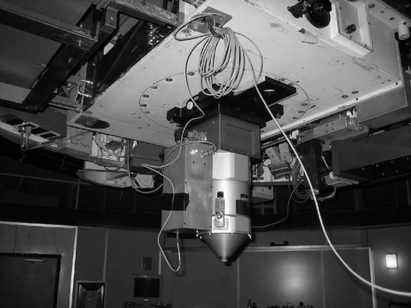
Figure 2: CAPSCam-S is shown mounted at the Cassegrain focus of the 2.5-m du Pont telescope at Carnegie’s Las Campanas Observatory in Chile.

The detector is mounted in our standard single-chip rectangular aluminum housing, coupled to an IR-Labs ND-2 cryostat. The control electronics box is mounted to the side of the dewar (Figure 2). The system is liquid nitrogen cooled, and has a hold time of approximately 13 hours.

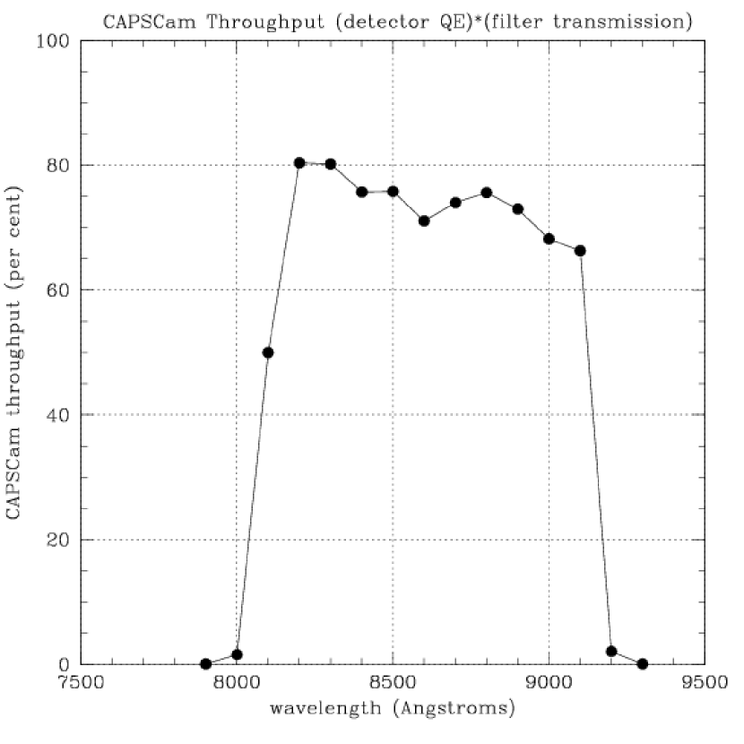
Figure 3: CAPSCam-S throughput in percent as a function of wavelength. The throughput is the product of the quantum efficiency of the Hawaii-2RG detector and the transmission function of the filter/window. CAPSCam is optimized for the study of M dwarf stars, with a bandpass of about 100 nanometers centered at about 865 nanometers.

The CAPSCam dewar window serves as the system passband filter, with a wavelength range of about 800 to 930 nm. Figure 3 illustrates the throughput of CAPSCam as a result of the combination of the Hawaii-2RG array and the filter/window. The filter/window was made with a multilayer coating on a 90 mm diameter $\lambda$/30 (peak to valley) fused-silica window from Barr Associates.

Two of us (GB and IBT) designed and built the electronics boards, and assembled both CAPSCams in our laboratories in Pasadena. The detector controller is a compact, 4-channel digital signal-processor-based system. It is a modified version of our BASE ccd control electronics, which is described in detail on the OCIW website. Tables 1 and 2 present more details about the CAPSCam read-out scheme, including the GW, FF, and overhead readout times.

One would normally operate the array without a shutter, using the built-in electronic reset function at the beginning of each FF or GW exposure. However, this would result in different sampling of the atmospheric turbulence by the wavefronts from the GW and FF stars, as the FF would continue to integrate during the time used for resetting and reading the GW. Hence a mechanical Uniblitz shutter and driver was purchased from Vincent & Associates, in order to synchronize the sky time for both the guide window and the full frame of the array. The optical path then consists solely of the primary and secondary mirrors, the shutter, the Barr filter/window, and the Teledyne array, eliminating optical distortions caused by any additional components.

CAPSCam-S camera was installed on the du Pont telescope in March 2007 (Figure 2) and has been in operation ever since, with several improvements having been made in the meantime. CAPSCam-S is controlled by a software graphical user interface (GUI) written by one of us (CB), which allows for convenient operation and monitoring of all of its functions. A detailed users manual for CAPSCam-S with a description of the GUI windows can be found on the Carnegie Observatories web pages.

The minimum integration time for the guide window is 0.2 sec, allowing CAPSCam to handle target M dwarf stars typically as bright as a V magnitude of $\sim$ 12 or an I magnitude of $\sim$ 9 without saturating the array. Saturated pixels show persistence at the level of a few hundred DN, which can last for several hours or more, even with repeated flushing of the array by taking dark frames. As a result, we try to avoid bright stars anywhere in the image. However, the low level of the persistence, and its confinement to a few pixels at the cores of saturated stars, means that it does not interfere with accurate astrometry of stars elsewhere in the field.

3 Target Star Sample Selection

Our top priority sample consists of 44 stars and brown dwarfs closer than 10 pc with spectral types later than M2.5, with another 26 dwarfs from 10 pc to 20 pc, for a total of 70 targets with known parallaxes within 20 pc. The majority of these targets have spectral type M5.5 or later. For observability, we require that the targets not saturate in our 0.2 s minimum integration time, i.e., have I magnitudes greater than $\sim$ 8.5. Only three of our targets have V magnitudes less than 12, which is a typical limiting magnitude for radial velocity surveys, even on large telescopes.

We restricted our sample to targets south of +16 deg declination in order to minimize airmass effects at the latitude of Las Campanas (-29 deg). Known close binary star systems have been avoided. We have supplemented our list with a number of M, L, and T dwarf targets from the 2MASS catalogs, which do not have parallax determinations yet. 10 have spectrophotometric parallaxes of 20 pc or less, 10 appear to lie beyond 20 pc, while 15 do not have even a spectrophotometric parallax. The very faintest L and T dwarfs (I $\sim$ 18 or more) have been dropped from consideration. After determining their parallaxes, those stars with distances greater than about 20 pc will also be dropped from further consideration, unless they show evidence for possibly having detectable companions. We intend to follow the best $\sim$ 100 targets for a decade or longer with CAPSCam-S on the du Pont.

4 CAPSCam Data Analysis Pipeline

We present here a brief description of the astrometric data pipeline developed at DTM specifically for CAPSCam. More complete details about the data pipeline and algorithms employed will be given in a forthcoming publication (see Anglada-Escudé et al., in preparation). We have also analyzed CAPSCam data with a completely separate data analysis pipeline developed by another of us (SBS), which has been used extensively in the Stellar Planet Survey (STEPS) astrometric program in the northern hemisphere on the Palomar 5-m telescope (Pravdo & Shaklan 1996). While the results obtained from the two approaches contain significant differences, these differences can be understood in terms of the different algorithms and data processing approaches used in the two pipelines.

CAPSCam data processing consists of two major steps: source extraction (or one night processing) and the astrometric iterative solution.

4.1 One Night Processing

A chosen image is used to create an astrometric template of the field for a given night. Some initial rejection of objects is done based on the roundness (ratio of the full-width-half-maximum [FWHM] of the point spread function [PSF] in the X and Y directions) and convergence properties of trying to find an initial rough estimate for the photocenter of each object (centroid). The 20 brightest objects (typically stars) are identified in every image and the rest of the objects are then located using the astrometric template. A fine centroiding algorithm is then applied and a catalog with the subpixel positions of all of the objects is obtained for all of the images of the field for a given night.

The centroiding algorithm consists of binning the PSF in the X and Y directions separately and fitting a one-dimensional PSF profile in each direction. Several different window sizes (apertures) are used on each object and the centroid position is found by averaging over all the apertures tried. This scheme has been compared to two-dimensional (2D) approaches (e.g., 2D Gaussian PSF fitting), and found to provide the most robust centroid determinations. The centroid determinations are very stable numerically, give the smallest scatter, and are insensitive to the discreteness of the sampling of the PSF.

When all the images for a given night are processed, the relative positions of all of the stars are compared, and the resulting scatter is used to estimate the centroid uncertainties for each star. Since we observe with telescope ditherings of $2^{{}^{\prime\prime}}$ in both X and Y, bad pixels and other Hawaii-2RG defects will move significantly and can be easily removed at this point. A final filtering of bad pixels and detector defects is then done to produce the final plate catalogs. The processing of each image generates a plate catalog, which contains a list of the X-Y-centroids and their associated uncertainties. One astrometric epoch typically then consists of between 20 to 80 plate catalogs obtained in a given night.

4.2 Astrometric Iterative Solution

Once images from a given field have been obtained on different nights spread over a long time baseline, an astrometric solution can be obtained and used to derive the positions, proper motions, and parallaxes of all the stars in each target field.

The astrometric solution is an iterative process. An initial catalog of positions is generated from a given plate, a transformation is applied to each plate catalog to match the initial catalog, and the apparent trajectory of each star is then fitted to a basic astrometric model. The initial catalog is updated with new positions, proper motions, and parallaxes and a subset of well-behaved stars is selected to be used as the reference frame. The selection of the reference stars is based on the number of successful observations and the median of the root-mean-square (RMS) of the residuals for the 100 brightest objects. A typical field contains around 40–50 of such stars. This process is then iterated a small number of times using only the reference stars for calibration purposes. The convergence of the astrometric solution is monitored by following the average RMS of the reference frame stars.

Since the number of targets followed and images generated by the CAPSCam planet search effort is large, the astrometric solution process has been designed to be fully automatic. Albeit structurally simple, some steps in this processing are algorithmically complex, especially those related to cross-matching, reference star selection, calibration weighting, astrometric model selection, etc. A more complete description of each of these steps will be given in Anglada-Escudé et al. (in preparation).

The initial catalog is matched to the NOMAD catalog (Zacharias et al. 2005), which contains USNO-B1 and 2MASS positions and colors of the brighter objects. This initial matching is required to better constrain the field rotation and plate scale, and to obtain the resulting astrometric positions in meaningful sky coordinates.

The final product is then an astrometric catalog containing five fitted astrometric parameters (effectively X and Y, the proper motions in X and Y, and the parallax), information about the number of observations employed, the RMS of the residuals per epoch, and the reduced $\chi^{2}$ of the solution for each star:

$$\bar{\chi}^{2}=\frac{1}{2N_{epochs}-N_{pars}}\sum^{N_{epochs}}_{i}\left[\frac{\left(x^{i}_{obs}-x_{model}\right)^{2}}{\sigma_{i}^{2}}+\frac{\left(y^{i}_{obs}-y_{model}\right)^{2}}{\sigma_{i}^{2}}\right],$$ (1)

where $N_{epochs}$ is the number of epochs, $N_{pars}$ is the number of model parameters to be fit, $x^{i}_{obs}$ and $y^{i}_{obs}$ are the measured positions of the star in a local coordinate system, $x_{model}$ and $y_{model}$ are the ones predicted by the best fit model, and the summation is over all epochs. Each observation is weighted using its own standard deviation $\sigma_{i}$.

Values of $\bar{\chi^{2}}$ greater than unity typically indicate the presence of uncalibrated systematic errors. These can occur for the target star as well as for the reference frame stars. The amount of this uncalibrated systematic error is obtained for each iteration by adding an error in quadrature to the estimated uncertainties derived from the calibration step until an effective $\bar{\chi}^{2}=1$ is obtained. This guarantees that the uncertainties in the parameters from the astrometric least squares solution are more realistic than the ones obtained using only the intra-night scatter. Despite the fact that part of any systematic error may come from chromatic effects, stars with less extreme colors than the red dwarf target stars show similar residuals (i.e., RMS deviations and $\bar{\chi^{2}}$) pointing to other sources of systematic errors related to the mechanical and optical stability of the telescope and detector on the scale of a few pixels. CAPSCam calibration observations are ongoing to try to clarify and identify the sources of such night-to-night and long-term systematic errors, which should add more or less in quadrature, with the hope of eventually reducing or eliminating these errors whenever possible. Systematic error sources include dome seeing, dust on the optics, minute changes in the optical alignment (depending on the temperature, humidity, or gravity angle), and the true effective photocenters of the individual pixels on the Hawaii-2RG.

Geometric calibration in the CAPSCam data pipeline accounts for differential optical aberrations with respect to the plate used as the initial catalog. We note that as long as we deal with the same instrument, only the time dependent part of the optical aberrations is relevant. This includes both atmospheric and instrumental-related optical distortions. The CAPS pipeline permits specifying the order of the polynomials to be used in the calibration. The zero order polynomial corresponds to a translational shift while the first order polynomial corrects for a small rotation and a shear. In the language of Zernike polynomials (see Noll 1975, his Table 1), the second order polynomials account for defocus and astigmatism. While the accuracy of the astrometric solution improves significantly if second order polynomials are used, we find that there is no significant improvement when using the third order ones as well; i.e., the third order Zernike aberration (coma) changes very little over the timespan of these CAPSCam-S observations.

5 Differential Chromatic Refraction

Ideally, astrometric observations are taken as the target star passes the meridian, in order to minimize atmospheric seeing effects and differential chromatic refraction (DCR, e.g., Pravdo & Shaklan 1996). Uncalibrated DCR leads to systematic errors because the photocenters of the target and reference stars will be refracted differently as the air mass changes. Pravdo & Shaklan (1996) found that DCR could be calibrated to about 0.13 milliarcsec for observations within 1 hour of the meridian and 45 degrees of the zenith with the Palomar 5-m. We intend to minimize the effects of DCR by using the same calibration technique for the du Pont and expect to be able to remove DCR to a level similar to that found to be possible at Palomar. The CAPSCam spectral bandpass has a FWHM of about 100 nanometers, centered on 865 nanometers, which also limits DCR effects for our red target stars and typically red reference stars.

In our first four years of du Pont observations (2003-2006), we used the Tek5 CCD camera to take Washington+DDO51 photometry (Geisler 1986; Majewski et al. 2000) of over 250 likely target stars (selected in part from Reyle & Robin 2004; Vrba et al. 2004; and Golimowski et al. 2004) and their reference stars, which is needed in order to remove the effects of DCR and to characterize the luminosity classes of the reference stars (i.e., distant giants are preferred and are identifiable with these filters; Majewski et al. 2000). Essentially all of the prospective target stars have sufficient reference stars within the 6.63 arcmin by 6.63 arcmin field of view of CAPSCam. We have also added Johnson B,V photometry (Johnson & Morgan 1953) for most fields, necessary for obtaining absolute parallaxes through reddening corrections. Hence, the characterization phase of our search is largely finished, though the occasional addition of new target fields to the planet search will require further Tek5 runs to obtain their colors.

At present, we apply a prototype of DCR correction in our CAPSCam data analysis pipeline which can be turned on or off. It is based on the colors from the NOMAD catalog (B,V from USNO-B1 and J,H,K from 2MASS). Ultimately, the chromatic corrections will be based on the Tek5 photometric determinations; this process is currently in development. Even with our crude DCR corrections we already see a distinct improvement of the quality of our astrometric solutions. Observations of a few target fields followed for about 6 hours through airmasses ranging from 1 to 3 are being used to estimate the DCR effects as a function of the TeK5 colors.

6 First Results with CAPSCam-S

The key objective of the CAPSCam program is achieving and maintaining an astrometric accuracy significantly better than a milliarcsecond for a decade or longer. The natural plate scale for CAPSCam-S on the du Pont is 0.194 arcsec/pixel, a scale that allows us to avoid introducing any extra optical elements into the system that would produce astrometric errors. We take multiple exposures with CAPSCam-S, typically 60 seconds for the full frame, with small variations (2 arcsec) of the image position (dithering), in order to average out uncertainties due to pixel response non-uniformity. We typically spend about one hour per field for each epoch. The ultimate goal is to achieve a precision of about 0.25 milliarcsec, and perhaps as low as 0.15 milliarcsec, which is the level of the atmospheric noise in one hour found by Pravdo & Shaklan’s (1996) Palomar 5-m study. Here we summarize our results to date.

The goal of this first paper is limited to giving concrete evidence of the astrometric performance of CAPSCam-S. We do not discuss important issues related to the choice of the reference frame or to zero–point parallax and proper motion corrections. Even still, it is remarkable that the proper motions obtained for the objects in the studied target field agree fairly well with those given in the USNO-B1 catalog (Monet et al. 2003), especially the reference stars.

6.1 NLTT 48256

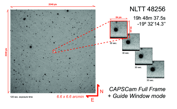
Figure 4: CAPSCam-S Full Frame image of Field 453, with NLTT 48256 located in the Guide Window.

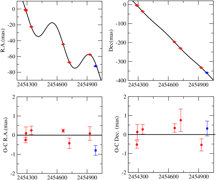
Figure 5: Top. R.A. (left) and Declination (right) shifts as a function of time for NLTT 48256. The parallax wobble can be clearly seen on the R.A. motion. Bottom. R.A. and Declination residuals (observed minus computed) with respect to the best fit model. All vertical axes are in milliarseconds (mas). The right-most data point is based on Guide Window and Full Frame data, while the others are Full Frame only. Use of the GW does not introduce any significant bias or jitter to the data.

We present here the performance of CAPSCam-S on Field 453 (Figure 4), which contains the target star NLTT 48256 (also known as LP 813-23 and as 2MASS J19483753-1932140). The target star is an M dwarf about which little is known. The field is rich in background objects ($\sim 400$), a few of which are brighter than the target. The previously reported properties of this star are given in Table 3. From the photometry, it is clear that it is a very red star ($V-K\sim 6.3$), most likely with a spectral type of M5V-M6V. Six epochs spread out over a 2 year period are presented here for this field (July 2007–June 2009, see Figure 5), so the parallax and the proper motion can be decoupled (for which only 3 epochs are required) and a preliminary discussion can be presented of the accuracy of the obtained solution, at least in a statistical sense. Table 4 gives the observing log information about the CAPSCam-S observations that were included in the analysis that follows.

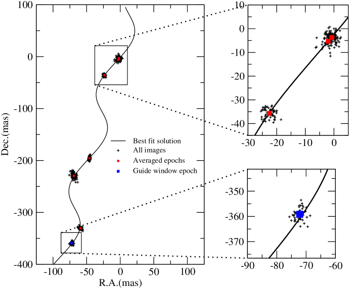
Figure 6: Motion of NLTT 48256 on the sky (R.A. vs. Dec.) in mas. On the top right, a zoom-in of the first two epochs is shown. The small crosses are the positions as measured from each individual image. The scatter is consistent with a standard deviation of $\sim 2$ mas per image in each direction, which is $\sim$ 1/100th of the pixel size of 0.194 arcsec. The bottom-most data point (and zoom-in) is based on Guide Window and Full Frame data, while the others are Full Frame only.

NLTT 48256 is faint enough for CAPSCam-S to use FF imaging without the need for the GW. The analysis that follows therefore is largely based on FF data for this field. However, we have also taken GW data on Field 453 in June 2009, with the GW centered on the target star. Forty images were obtained on two separate nights. The resulting astrometric accuracy of the combined nights is shown in Figures 5 and 6, though the GW epoch was not included in the solutions given in Tables 5 and 6. Figures 5 and 6 show that usage of the GW mode does not introduce a significant bias into the astrometric measurements, and provides a precision comparable to that of the FF mode.

6.2 Achromatic solution

No color correction is applied in this first case. After excluding poorly-behaved stars in the first iteration, the reference frame still contains 39 objects that appeared in at least $90\%$ of the frames. These 39 objects define a robust reference frame with a median RMS per epoch of 1.1 milliarcsec (mas). The astrometry of the poorly-behaved stars is also obtained, but they are not used in the calibration matching step.

The RMS of the solution for the target star is $0.38$ mas/epoch, which is a proxy for the long-term stability of the instrument. Since our desired target star accuracy is $\sim 0.25$ mas/epoch, evidently further work will be required to try to reach this figure. Using the method described in the previous sections, we estimate the amount of systematic error, finding that it is $0.3$ mas/epoch. Clearly the systematic error is a significant source of the scatter in the residuals (see Figure 5, bottom panels). Similar values are achieved for a significant number of reference stars in the field, providing a robust double-check on the quality of the entire astrometric solution. The residuals appear to be somewhat larger in Dec. than in R.A., and we are investigating possible sources of this apparent difference.

The target star does not show any excess in the post-fit residuals when compared to other stars in the field with similar magnitude. In fact, the RMS of the target star is slightly smaller than the average. Since the target star is located at the center of the field, where the optical distortions are less severe, this is not totally unexpected.

The final astrometric solution for the target star is given in Table 5. The proper motion and parallactic motion of NLTT 48256 are displayed in Figures 5 and 6. The resulting parallax is $\sim 17$ mas, which puts the target star at a distance of $58$ pc, considerably beyond our distance cut-off of about 10 pc. However, this star will be kept in the observing program in order to monitor the long-term stability of CAPSCam-S and to support our search for sources of systematic errors. Claims for astrometic planet detections are best supported by observations showing that other target stars are not being similarly perturbed (so-called “flat-liners”, R. P. Butler, personal communication), so Field 453 will continue to provide an invaluable check on the short- and long-term astrometric accuracy of CAPSCam-S.

6.3 Chromatic solution

The same procedure as above has been applied using $R-J$ color as a variable in the calibration step, which is the color most closely related to the slope of the spectral energy distribution in the CAPSCam working band. The number of useful reference frame stars drops to 35 in this case because only stars with known R and J colors are used. The RMS of the astrometric solution for the target star decreases to $0.35$ mas/epoch, showing a slight improvement in the accuracy. We note that the parallaxes determined with and without the chromatic correction are incompatible at the several $\sigma$ level. This is caused by the correlation of the DCR with the parallax factor, which introduces a small bias into the parallax estimation. Since our current version of the DCR correction is only a prototype, we expect a small but significant increase in the accuracy and a better decoupling of the true parallax from color dependent effects once we are able to derive a solution with the full Tek5 photometric colors.

6.4 Search for periodic signals

Once the main astrometric solution is finished, we can fit the plate motion of the target star with an astrometric model including a Keplerian component. However, with effectively only five epochs (i.e., 10 measurements of either X or Y), there is not enough information to solve for a fully Keplerian orbit plus the astrometric solution. Hence, this exercise should be considered purely as an academic one. We can then run a Least Squares periodogram routine, which consists of fitting for each orbital period $P$ sampled a linearized astrometric solution with a circular orbit in an arbitrary orientation, i.e.,

$$X_{\alpha} = X_{0}+\mu^{*}_{\alpha}\left(t-t_{0}\right)+\Pi p_{\alpha}\left(t\right)+A\sin 2\pi/P+B\cos 2\pi/P$$ (2)

$$Y_{\delta} = Y_{0}+\mu_{\delta}\left(t-t_{0}\right)+\Pi p_{\delta}\left(t\right)+C\sin 2\pi/P+D\cos 2\pi/P$$ (3)

where the offsets $X_{0}$ and $Y_{0}$, proper motions $\mu^{*}_{\alpha}$ and $\mu_{\delta}$, parallax $\Pi$ and the orbital coefficients A,B,C and D are solved simultaneously for each test period $P$. The functions $p_{\alpha}(t)$ and $p_{\delta}(t)$ are called the parallax factors. They are the projections of the parallactic motion in R.A. and Declination in the direction of the star. The barycentric instant of observation is $t$ and the reference epoch at which the astrometric parameters are defined is $t_{0}$.

In order to maximize the sensitivity of our planet search, we have developed a Least Squares periodogram approach that may perform better than other proposed methods, such as the Joint Lomb-Scargle periodogram proposed by Catanzarite et al. (2006). Our Least Squares minimization solves simultaneously for the signal, parallax, proper motion, and two small offsets in each direction. All of these parameters are intrinstic to the astrometric measurements, and can correlate spuriously with the sampling cadence and the true signal, leading to incorrect identification of candidate periods. The Least Squares approach remains linear in all the free parameters if only astrometric data is involved (see, e.g., Pourbaix 1998), which makes it computationally efficient and numerically well-behaved. Black & Scargle (1982) were the first to point out that the coupling between the reflex signal and proper motion will lead to underestimates of both the period and the amplitude of the signal, even when the data span the entire period of the signal. We go one step further, and include both the proper motion and the parallax during our period search, ensuring that we recover the correct orbital period from the start.

In this context, we note that the Lomb-Scargle periodogram is a special case of Least Squares minimization (Cumming 2004), where the Least Squares minima (or the peaks of the periodogram) identify the correct periodicities when the true signal is close to a sinusoid (see Frescura et al. 2008). This point was first made by Scargle (1982). A Lomb-Scargle periodogram works very well with radial velocity data, where the only relevant parameter not related to the periodic motion is a constant offset. This performance breaks down, however, for astrometric data, due to the time dependence of the proper motion and the parallax. If the true signal’s period is well-sampled, the Lomb-Scargle periodogram provides an answer close to the correct one (Traub et al. 2009), but its statistical interpretation in terms of significance and confidence level is unclear. We are continuing to investigate the comparative performance of both approaches when applied to astrometric data, but for the purposes of this initial paper, we limit ourselves to the Least Squares approach.

The purpose of the Least Squares periodogram is to find an initial set of astrometric parameters that can be used as a first approximation for a fully Keplerian solution that minimizes some merit function (i.e., $\chi^{2}$). The Least Squares periodogram approach allows the weighting of each observation properly at the initial period-search level, and provides all the parameters of the best-fit circular orbit (via the Thiele-Innes elements), which can be used as initial values to solve the fully nonlinear Kepler problem (e.g., Wright et al. 2009).

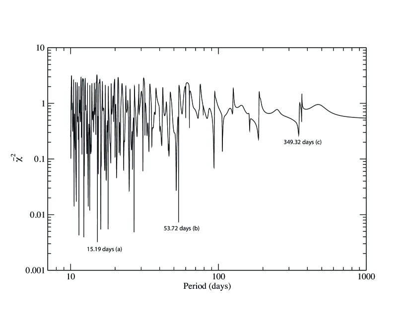
Figure 7: Best $\bar{\chi}^{2}$ as a function of the period (periodogram) for NLTT 48256. The minima represent the candidate periods. Since the number of observations is still small, most of the minima are spurious and can be attributed to well-known issues related to poor data sampling (see Figure 8).

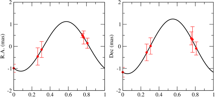
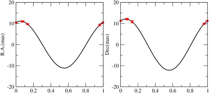
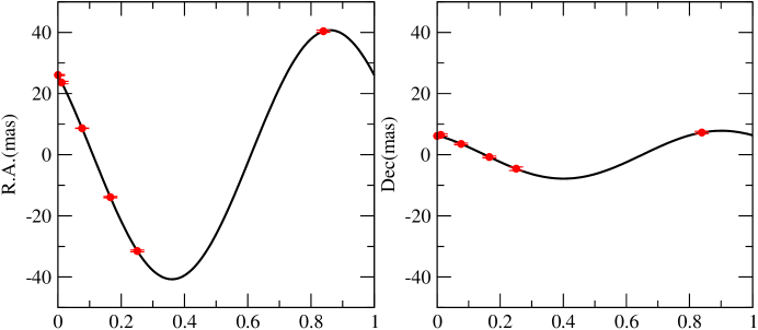
Figure 8: False minima in the periodogram for NLTT 48256 can lead to spurious solutions. Top. Best fit period, showing R.A. and Dec. as functions of the orbital phase, for $P\sim 15$ days. The $\bar{\chi}^{2}$ is much smaller than 1 because the number of parameters being fitted almost matches the number of observations. Center. Aliasing with the observing cadence ($P\sim 54$ days). All the data appears to be concentrated on a small orbital phase. Bottom. Coupling with the parallax. Here the apparent period is $P\sim 349$ days, about one Earth year. The parallax obtained for this solution is $-25$ mas, clearly illustrating that this spurious signal is due to the strong correlation with the parallax period.

If one calculates the $\bar{\chi}^{2}$ as a function of the period (i.e., draw a periodogram, see Figure 7), the minimum $\bar{\chi}^{2}$ is the best circular model fitting the data. Currently, the number of measured parameters is comparable to the number of unknowns, and so a large number of artificial least squares minima with $\bar{\chi}^{2}$ much smaller than 1 appear in the periodogram. However, this periodogram does give information about the most important orbital phases that have to be sampled in order to eliminate spurious signals, as shown in Figure 7. The best period for NLTT 48256 is at $15.19$ days and has a semi-amplitude of $1.2$ mas. However, the model clearly fits the data too well, as shown in the phased representation of the best orbit in Figure 8 (top). Other minima in the periodogram are due to the aliasing of the noise with the sampling cadence (Figure 8, center) and the coupling of the astrometric motion with natural periodicities, such as the parallax (Figure 8, bottom). External constraints can be used to suppress such unrealistic least squares minima, however the best strategy is simply taking more data and optimizing the cadence to minimize the effects of the discrete sampling cadence.

In general, the minimum number of observations needed to constrain with confidence an orbital model is a complicated function of the number of observations, signal-to-noise ratio, spacing of the observational epochs, orbital period and eccentricity, and the choice of the statistical tests used to choose the best orbital model (e.g., Sozzetti 2005; Casertano et al. 2008; Ford 2008; Cumming et al. 2008; Wright & Howard 2009). However, a lower bound on the number of observational epochs required to solve for a planetary companion can be determined simply from linear algebra theory: at least $n$ independent observations are needed to solve a system with $n$ unknown factors. For a circular Keplerian orbit, there are a total of 10 free parameters in the astrometric solution for the orbit, proper motion, and parallax, while for an eccentric orbit, there are 2 more free parameters (eccentricity and the argument of periastron), for a total of 12 free parameters. For a circular orbit, then, at least 5 observational epochs in two coordinates (R.A. and Dec.) are required for a solution, and at least 6 epochs for an eccentric orbit. Clearly, such minimal solutions must be considered dubious, and require additional epochs for their validity to be properly assessed. We expect that at least 10 or 12 epochs (20 or 24 measurements in R.A. or Dec.) will be necessary to constrain circular or eccentric orbits, respectively. In cases where additional information is available (e.g., radial velocities, or catalog proper motions), these estimates might be relaxed somewhat.

7 STEPS Data Analysis Pipeline

The STEPS data reduction process (Pravdo et al. 2004) begins by extracting square regions containing the target and reference stars from the raw frames and organizing them into a single file, from which positions for all stars are determined. The cross-correlation of the reference star positions relative to the target star is determined by the weighted slope of the phase of the Fourier Transform of the images after summing them into horizontal and vertical distributions. This algorithm is insensitive to the background level, robust against changes in the shape of the point spread function (PSF), and maintains a signal-to-noise ratio comparable to matched filtering. Centroiding is then performed, and a preliminary astrometric solution is obtained by fitting a conformal six-term (three per axis) transformation for each CCD frame to a reference frame. The transformation is then applied to the target star as well, allowing the target star position to be measured relative to the surrounding reference stars. An automated program then searches for frames whose astrometric noise is above a user-defined threshold. Generally, the threshold can be set to be very high, because the major cause of unusable data is missing reference stars or selection of the wrong star. After removal of the bad frames, the conformal transformation is run again to form an intermediate astrometric solution.

The DCR effect is proportional to the tangent of the zenith angle and leads to a linear shift in right ascension and a parabolic shift (relative to the meridian position) in declination. The relative DCR coefficient for each star is determined empirically by fitting the right ascension shift. A single coefficient for each star is defined as the weighted average of the nightly coefficients, used to adjust the centroid positions, and the conformal transformation is rerun once again. The position of the target star relative to the reference frame is then known for that night.

The final STEPS processing step is to fit the motion of the target star to a model of the its parallax, proper motion, and radial velocity. STEPS uses relative, rather than absolute, proper motions and parallaxes. The USNO subroutine ASSTAR is used to compute the astrometric wobble, and the NAIF subroutine CONICS is used to determine the position and velocity of a suspected companion from an assumed set of elliptic orbital elements, which are then varied in order to find the best fit.

The analysis of NLTT 48256 using the STEPS pipeline is in good agreement with the analysis obtained using the CAPSCam data reduction scheme. However, the intra-night scatter and corresponding single epoch uncertainties are larger using the STEPS pipeline. We attribute this to the STEPS centroiding approach, which requires a finer sampling of the stellar PSF than is obtained using CAPSCam-S – the seeing-disk to pixel ratio is about 15 to 20 with the STEPS camera on the Palomar 5-m telescope, while the ratio is about 5 for CAPScam-S on the 2.5-m du Pont.

It is also significant that the reference stars used in the two analyses are not exactly the same. We attribute the discrepancy in the obtained proper motions to these differences. In spite of these differences, both astrometric solutions agree to within the errors (see Table 5). A refined centroiding algorithm using an analytic approximation of the PSF is being implemented on the STEPS pipeline in order to achieve improved compatibility with the CAPSCam pipeline. Table 6 presents the R.A. and Dec offsets as a function of time for those who may wish to try their own fit to this CAPSCam-S data.

8 Comparison With Other Ground-Based Programs

Considerable progress has been made in the adaptation of CCDs to the field of astrometry. Most notable is its application in an astrometric instrument called STEPS, which has been used at Keck and at the Palomar 5-m telesope (Pravdo & Shaklan 1996). STEPS is able to achieve high precision (approximately 0.25 to 0.5 milliarcsec) on 30 minute exposures of intrinsically faint M dwarfs in fields with bright, well-distributed reference stars. STEPS has detected a low-mass M6-M8 binary companion to the M dwarf GJ 164, with a noise floor of $\sim$ 1 milliarcsec (Pravdo et al. 2004). STEPS has also found low mass companions to the M dwarfs GJ 802 (Pravdo, Shaklan, & Lloyd 2005) and G78-28AB and GJ 231.1BC (Pravdo et al. 2006). Most recently, STEPS appears to have achieved the first astrometric discovery of a planet, finding evidence for a $\sim$ 6 Jupiter mass planet candidate with an orbital period of 0.744 year around the M8 star VB10 (Pravdo & Shaklan 2009).

Bartlett, Ianna, & Begam (2009) summarized the results of their three years of observations of thirteen nearby (within 25 pc) stars in the University of Virginia Southern Parallax Program. They were able to achieve parallaxes with errors of less than 3 milliarcsec for these stars, all early M dwarfs, using a minimum of at least 50 observational epochs. One star, LHS 288, appears to exhibit a wobble indicative of a very low mass companion, and this star appears in the CAPSCam-S observing list as well.

Henry et al. (1997, 2006) have been prolific in finding the closest stars and in searching the 91 closest red and white dwarf stars for low mass companions, using 1m-class telescopes and existing CCDs at Cerro Tololo (ASPENS). The ASPENS program typically achieves astrometric accuracies of about 1.5 milliarcsecs. The median seeing at Cerro Tololo is about 0.95 arcsec, compared to 0.6 arcsec on Las Campanas (Persson et al. 1990), both measured at 0.5 microns. As a result, and because of the larger aperture (2.5-m), better plate scale, and smaller optical distortions on the du Pont, we expect our survey to achieve better long-term astrometric accuracies.

Bower et al. (2009) used the Very Large Array (VLA) to perform a radio astrometry survey of 172 active M dwarfs within 10 pc. They were able to place upper bounds on the presence of any planetary companions of no more than 3 to 6 Jupiter masses orbiting at $\sim$ 1 AU. The VLA survey typically yielded milliarcsecond resolution, though for four stars that were observed at multiple epochs, the RMS residuals were $\sim$ 0.2 milliarcsecs.

Adaptive optics (AO) has been used on the Palomar 5-m telescope to improve the astrometric performance, with accuracies achieved as good as 0.1 milliarcsec over 2 months (Cameron, Britton, & Kulkarni 2009). The FORS1 camera on one of the Very Large Telescope (VLT) 8-m telescopes has achieved astrometric accuracies of 0.2 to 0.3 milliarcsecs per single measurement (Lazorenko et al. 2007).

Interferometry has the greatest ultimate potential for astrometric detection of extrasolar planets (Shao & Colavita 1992). The Palomar Testbed Interferometer (PTI), with 0.4-m aperture siderostats, has been used primarily for interferometer instrumentation and software development (Colavita & Shao 1994). The main limitation of the PTI is that it can only use one reference star at a time, and that one star must be quite bright and very near to the target. Thus the PTI does not have a significant planet survey capacity, even though it has demonstrated an astrometric accuracy of about 0.1 milliarcseconds over a period of a few days. The PTI has been successfully employed in very high precision studies of several double stars (e.g., Boden et al. 1999; Boden & Lane 2001).

The Palomar AO, VLT/FORS1, and PTI experiments have thus demonstrated high precision, but only over very short time baselines (days to months) compared to our results to date (spanning several years of CAPSCam-S data). Given the need for long term stability (by definition) in an astrometric planet search, we believe that CAPSCam is well-suited for making significant astrometric discoveries.

The Very Large Telescope Interferometer (VLTI) will also be capable of astrometric planet searches. The VLTI plans to begin astrometric observations in 2010 with four auxiliary (1.8-m) telescopes forming the PRIMA interferometer and to achieve an astrometric accuracy of about 0.03 milliarcsecs. However, late M, L, and T dwarfs will be too faint for interferometric astrometry on $\sim$ 100-m baselines with 1.8-m telescopes and with bandpasses limited by the difficulty of achieving achromatic fringes. In fact, the PRIMA planet search of 100 to 200 stars is planned only for target stars that are brighter than K = 12 to 14 (J. Setiawan, 2004, private communication), limiting this search to stars earlier than early M type.

Radial velocity surveys have been by far the most successful and valuable of all the planet-search techniques. However, these spectroscopic searches typically require a high flux of optical stellar photons in order to achieve velocity precisions of a few m/sec, and consequently they have been generally limited to target stars brighter than about V = 11 (R. P. Butler, private communication, 2008). Our planned astrometric search will be complementary to the spectroscopic surveys of low mass stars (e.g., Butler et al. 2004), as our targets are typically no brighter than V = 13. For example, the HARPS GTO program (PI: Michel Mayor) on the La Silla 3.6-m telescope includes only 10 stars with spectral types later than M5 and none as late as M7. The Carnegie-California search has a similar number of very late type stars (Wright et al. 2004). While radial velocity surveys are intrinsically better suited for discovering planets in short-period orbits (Figure 9), astrometry is better suited for long-period orbits, requiring that the CAPSCam planet search be at least a decade-long effort. Ideally, astrometry and radial velocity could observe the same target stars, so that astrometry could remove orbital inclination ambiguity of radial velocity observations. A few planets have been discovered by radial velocity that are close enough, faint enough, and located far enough south to be prime candidates for CAPSCam astrometry.

9 Comparison With Space-Based Programs

The European Space Agency (ESA) Hipparcos satellite (1989-93) and the resultant catalog comprise the most successful astrometric effort in history. Hipparcos obtained the parallaxes of nearly 120,000 stars with a median precision of about 1 milliarcsecond. Hipparcos’ ability to detect an astrometric planet perturbation was limited primarily by the mission’s duration of only 3.36 years and by its annual precision of approximately 2 milliarcseconds.

Astrometric efforts with the Hubble Space Telescope (HST) have been almost entirely confined to use of the interferometers of the fine guidance system (FGS) instead of HST’s CCD cameras. The resulting studies are among the highest precision (approximately 0.5 milliarcsec) planet searches to date (Benedict et al. 1999). Unfortunately these searches were of limited duration. The FGS has also been used to place an upper limit on the mass of the short-period companion to 55 Rho¹ Cancri of about 30 $M_{Jup}$ (McGrath et al. 2002), a result that differed considerably from the Hipparcos evidence for a wobble large enough to require the presence of an M dwarf companion with a mass of 126 $M_{Jup}$. The FGS measurements, with an accuracy of about 0.3 milliarcseconds, rule out the Hipparcos claim. More importantly, Benedict et al. (2002) used the FGS to determine the mass of the outermost planet of the GJ 876 system to be $1.9M_{Jup}$, the first time that astrometry has determined the mass of an extrasolar planet. The low mass of the GJ 876 primary star ($0.32M_{\odot}$) enabled this detection, along with knowing basic orbital parameters from the original spectroscopic detection of the star’s planets. While the FGS evidently can be a potent astrometric instrument, the difficulty of obtaining precious HST time for lengthy astrometric surveys limits its use to following up on particularly promising spectroscopic detections, such as GJ 876.

10 Conclusions

Our analysis of the target star NLTT 48256 shows that an astrometric accuracy better than $0.4$ mas can be obtained over a time scale of several years with CAPSCam-S on the du Pont 2.5-m. Our preliminary DCR correction indicates that full differential chromatic corrections will be required in our data pipeline if accuracies below $0.3$ mas/epoch are to be achieved. We are presently working in this direction. Such a long-term accuracy would probably be the best accuracy that could be achieved with seeing-limited observations over a time-scale of many years on a 2.5-m-telescope, and would be the result of the combination of a very stable instrument with a strict data processing scheme.

A Jupiter-mass planet on a Jupiter-like orbit around a solar-mass star produces an astrometric wobble of the primary star of 2 milliarcsec (measured peak to valley) when viewed from a distance of 5 pc. Thus an astrometric accuracy of (plus or minus) 0.25 milliarcsec would allow the detection of such a planetary companion with a signal-to-noise ratio of 4. For lower mass stars, the nominal astrometric detection limit drops to proportionately lower planet masses. Brown dwarf companions at similar orbital distances will be considerably easier to discover.

Optical Doppler surveys have observed about 200 different M-type stars. These are mainly of spectral type earlier than M3, due to the constraint of needing high V-band magnitudes. Cummings et al. (2008) find a statistically significant deficit of planets with masses between 0.3 and 10 Jupiter masses and with orbital periods $<$ 2000 d around M-dwarfs relative to FGK-dwarfs – a gas giant planet fraction of 2% rather than 7.5% for these relatively short ($\sim$ 5 yr) orbital periods. Investigations of the period-mass relation for M stars are still impossible due to the small number of detected planets. The planet fraction around stars and brown dwarfs with mass $<0.25M_{\odot}$ is largely unprobed. Doppler searches of small samples of young stars have so far revealed an 18 Jupiter-mass object around a brown dwarf (Cha H$\alpha$ 8; Joergens & Muller 2008). Optical Doppler surveys have targeted very few of these faint stars because integration times are prohibitively large, and infrared Doppler surveys are in their infancy. Direct imaging studies can only search for planets widely separated from young brown dwarfs (e.g., 2MASS1207; Chauvin et al. 2004). Astrometry searches closer in, and removes the orbital inclination ambiguity of Doppler surveys. Hence we believe that by targeting late M, L, and T dwarfs for astrometric monitoring for a decade or more, CAPSCam will make an important contribution to the census of planetary systems.

We believe that a sample of around 100 stars is sufficiently large to ensure a reasonable statistical measure of the frequency of long-period gas giant planets (and binary companions) around late M and later type dwarfs, companions with orbital periods long enough to permit habitable rocky planets to orbit these stars on shorter period orbits. M dwarfs have recently been recognized as attractive targets in the search for life beyond the Solar System (Segura et al. 2005; Tarter et al. 2007), yet late M dwarfs are not being studied by optical Doppler surveys in any great number. While CAPSCam will not be able to detect habitable terrestrial planets, we will be able to point the way for searches by future ground- and space-based telescopes designed to discover new Earths around the closest stars. In fact, the report of the Exoplanet Task Force (Lunine et al. 2008) specifically calls for planet searches around M dwarfs to be a fast-track effort for ground-based and existing space telescopes (see their Figure 1).

We thank Paul Butler, Sandy Keiser, and Dave Monet for their key contributions to this effort, and Wendy Freedman, Mark Phillips, and Miguel Roth for their steady support of this ambitious program at Las Campanas. Oscar Duhalde, Javier Fuentes, Gastón Gutiérrez, Herman Olivares, David Osip, Fernando Peralta, Frank Pérez, Patricio Pinto, and Andrés Rivera have provided valuable assistance at Las Campanas. We thank the referee as well, whose comments have helped to improve the paper. This work has been supported in part by NSF grants AST-0352912 and AST-0305913, NASA Planetary Geology and Geophysics grant NNX07AP46G, NASA Origins of Solar Systems grant NNG05GI10G, and NASA Astrobiology Institute grant NCC2-1056. This research has made use of the SIMBAD database, operated at CDS, Strasbourg, France.

Table 1: CAPSCam array readout times (in seconds).

FF times (2048$\times$2048)
FF-flush time:	2.146
FF-read time:	8.397
GW times
GW-pixel size:	32x32	64x64	128x128	256x256
GW-flush time:	0.003	0.010	0.036	0.137
GW-read time:	0.009	0.034	0.133	0.528

Table 2: CAPSCam sample exposure sequence for 60 s FF, 1 s GW (64$\times$64).

time (s)	Action
0.000	FF flush start
2.146	FF 1st read start
10.543	FF read done (wait until next full second)
11.000	GW flush start
11.010	GW 1st read start (exposure 1)
11.044	open shutter
12.044	close shutter, wait 50 ms
12.094	GW 2nd read start (exposure 1)
12.128	GW read done (wait until next 0.1 second)
12.200	GW flush start
12.210	GW 1st read start (exposure 2)
12.244	open shutter
13.244	close shutter, wait 50 ms
13.294	GW 2nd read start (exposure 1)
13.328	GW read done (wait until next 0.1 second)
13.400	GW flush start
…	elapsed time = $11+60*1.2=83$
83.000	50ms wait for shutter to close
83.050	FF 2nd read start
91.477	FF 2nd read done

Table 3: Catalog information on NLTT 48256. Proper motion and coordinates are from the NLTT catalog (Salim & Gould 2003) and color is from the NOMAD catalog (USNO-B1 + 2MASS, Zacharias et al. 2005).

Reference epoch JD 2000
RA	19 48 37.5
Dec	$-$19 32 14.3
$\mu$RA	$-$38 $\pm$ 20 mas/yr
$\mu$Dec	$-$187 $\pm$ 20 mas/yr
R	16.84
R$-$J	3.63

Table 4: Log of observations of Field 453. The SNR on NLTT 48256 is always over 1000 and the faintest reference frame star has a typical SNR of 200-300. Exposure times are given in seconds while the seeing is in arcseconds.

Date	FF Exptime	GW Exptime	# FF Images	Seeing	Airmass
2007 Jul 04	60	–	90	0.9	1.02
2007 Jul 08	100	–	36	1.2	1.02
2007 Aug 31	60	–	60	0.9	1.01
2008 Jul 14	30	–	80	0.8	1.03
2008 Sep 12	30	–	80	1.0	1.16
2009 Apr 10	60	–	26	0.7	1.14
	45	–	15	0.7	1.06
2009 Jun 01	120	30	20	0.9	1.02
2009 Jun 04	120	30	20	0.8	1.02

Table 5: Astrometric solution for NLTT 48256. Reference epoch is August 31, 2008 or Julian Date: 2454343.558125. In all cases there are 5 effective epochs and 366 images.

	CAPSCam		STEPS
	Achromatic	Chromatic
RA	19 48 37.488	19 48 37.488
Dec	$-$19 32 15.926	$-$19 32 15.925
muRA(mas/yr)	$-$40.04 $\pm$ 0.13	$-$39.99 $\pm$ 0.12	$-$41.7	(+1.10 $-$1.00)
muDE(mas/yr)	$-$187.71$\pm$ 0.13	$-$187.66 $\pm$ 0.12	$-$188.8	(+1.10,$-$1.00)
par(mas)	17.80 $\pm$ 0.15	16.69 $\pm$ 0.14	17.37	(+0.49,$-$0.46)
RMS(mas/epoch)	0.38	0.35	1.50

Table 6: Astrometric shifts of NLTT 48256 in local plane coordinates, uncertainties, and postfit residuals after fitting an offset, parallax, and proper motion only. All angles given in milliarcseconds (mas).

Julian Date	RA Shift	Dec Shift	RA unc	Dec unc	O-C RA	O-C Dec
2454285.726960	-1.566825	-3.984330	0.143	0.205	-0.008	-0.801
2454289.733512	-2.872852	-5.162385	0.304	0.383	0.187	0.271
2454343.589780	-22.608162	-35.169847	0.184	0.263	-0.117	0.566
2454661.673801	-45.457509	-197.023902	0.085	0.259	-0.030	-0.054
2454722.625970	-66.343008	-230.239554	0.218	0.472	-0.070	0.883
2454928.216687	-59.445586	-332.217484	0.295	0.335	0.090	-0.472

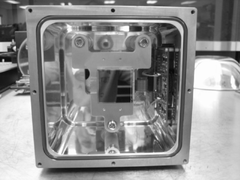
Figure 1: The Teledyne Hawaii-2RG array can be seen mounted in the center of CAPSCam-N, shown here with the Barr Associates filter/window removed. The Hawaii-2RG array is approximately 2” by 2” in size.

Figure 9: Discovery space for gas giants and hot super-Earths (solid dots) and brown dwarfs (unlabelled open circles) found by Doppler spectroscopy. Data points plotted are from the IAU Working Group on Extrasolar Planets (WGESP) web site (http://www.dtm.ciw.edu/users/boss/planets.html), which is complete up to August 2006, augmented with the most recent hot super-Earths. Nearly all of the host stars are G dwarfs, though the hot super-Earths tend to be found around early M dwarfs. Objects with masses above 13 Jupiter masses are considered by the WGESP to be brown dwarfs, not planets, though this plot represents objects with m sin $i$ values below 20 Jupiter masses as planets. The oblique dashed line illustrates the dependence of the sensitivity limit for spectroscopic detections on semimajor axis (for a signal-to-noise ratio of four for 2.5 m/s Doppler precision and a solar-mass host star), while the oblique solid and dotted lines represent the limits for astrometric detections with 0.25 milliarcsec accuracy and a signal to noise ratio of four, for a late M dwarf target star at distances of 5 pc and 15 pc, respectively.