A Fresh Look at Coding for
$q$-ary Symmetric Channels

Abstract

This paper studies coding schemes for the $q$-ary symmetric channel based on binary low-density parity-check (LDPC) codes that work for any alphabet size $q=2^{m}$, $m\in\mathbb{N}$, thus complementing some recently proposed packet-based schemes requiring large $q$. First, theoretical optimality of a simple layered scheme is shown, then a practical coding scheme based on a simple modification of standard binary LDPC decoding is proposed. The decoder is derived from first principles and using a factor-graph representation of a front-end that maps $q$-ary symbols to groups of $m$ bits connected to a binary code. The front-end can be processed with a complexity that is linear in $m=\log_{2}q$. An extrinsic information transfer chart analysis is carried out and used for code optimization. Finally, it is shown how the same decoder structure can also be applied to a larger class of $q$-ary channels.

I Introduction

The $q$-ary symmetric channel ($q$-SC) with error probability $\epsilon$ takes a $q$-ary symbol at its input and outputs either the unchanged input symbol, with probability $1-\epsilon$, or one of the other $q-1$ symbols, with probability $\epsilon/(q-1)$. It has attracted some attention recently as a more general channel model for packet-based error correction. For very large $q$, its appropriately normalized capacity approaches that of an erasure (packet loss) channel. In the following, we will only consider channel alphabets of size $q=2^{m}$ with $m\in\mathbb{N}$.

The capacity of the $q$-SC with error probability $\epsilon$ is

$$C_{\text{$q$-SC}}=m-h(\epsilon)-\epsilon\log_{2}(2^{m}-1)$$

bits per channel use, where $h(x)=-x\log_{2}x-(1\!-\!x)\log_{2}(1\!-\!x)$ is the binary entropy function. Asymptotically in $m$, the normalized capacity $C_{\text{$q$-SC}}/m$ thus approaches $1\!-\!\epsilon$, which is the capacity of the binary erasure channel (BEC) with erasure probability $\epsilon$.

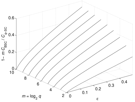
Figure 1: Relative capacity loss $1-\frac{mC_{\text{BSC}}}{C_{\text{$q$-SC}}}$ of marginal BSC vs. $q$-SC.

Figure 2: Normalized capacity of $q$-SC vs. marginal BSC (error probability $\epsilon=0.1$).

Recent work [1, 2, 3, 4, 5] has shown that it is possible to approach $C_{\text{$q$-SC}}$ for large alphabet sizes $q=2^{m}$, with symbols of hundreds to thousands of bits, and complexity $O(\log q)$ per code symbol. The focus of the present work is on smaller $q$, with symbols of tens of bits at most, although the presented coding techniques will work for any $q=2^{m}$.

The $q$-ary channel input and output symbols will be represented by binary vectors of length $m$. Hence a simplistic coding approach consists in decomposing the $q$-SC into $m$ binary symmetric channels (BSCs) with crossover probability

$$\epsilon_{\text{BSC}}=\frac{q\epsilon}{2(q-1)}=\frac{\epsilon}{2(1-2^{-m})},$$ (1)

which have capacity $C_{\text{BSC}}=1-h(\epsilon_{\text{BSC}})$ each.

We briefly study the normalized capacity loss, $\Delta=C_{\text{$q$-SC}}/m-C_{\text{BSC}}$, which results from (wrongly) assuming that the $q$-SC is composed of independent BSCs. For fixed $m$, we have $\lim_{\epsilon\to 0}\Delta=0$; so using binary codes with independent decoders on the $m$-fold BSC decomposition might be good enough for small $\epsilon$ (e.g. $\epsilon<10^{-3}$). However, Figure 1 shows that the relative capacity loss ${m\Delta}/{C_{\text{$q$-SC}}}=1-{mC_{\text{BSC}}}/{C_{\text{$q$-SC}}}$ increases close to linearly in $\epsilon$. For fixed $\epsilon$, we have $\lim_{m\to\infty}\Delta=h(\epsilon/2)-\epsilon$, which can be a substantial fraction of the normalized $q$-SC capacity (e.g., for $\epsilon=0.1$, $h(\epsilon/2)-\epsilon=0.19$). Figure 2 shows that already for small $m$, the $q$-SC capacity is substantially larger than what can be achieved with the BSC decomposition. Clearly, there is a need for coding schemes targeted at “large” $\epsilon$ (say $\epsilon>10^{-1}$), but moderate $m$ (say $2\leq m<20$), which are not that well handled by methods for large $q$. For example, for using verification-based decoding the symbols should have between $m=32$ bits for short codes (block length $10^{2}\ldots 10^{3}$) and $m=64$ bits for longer codes (block length $10^{4}\ldots 10^{5}$) [1].

One example application, which also motivated this work, is Slepian-Wolf coding of $q$-ary sources with a discrete impulse-noise correlation model, using $q$-SC channel code syndromes as fixed-rate (block) source code. This can then be used as a building block for a Wyner-Ziv coding scheme, where $q$ is the number of scalar quantizer levels, or for fixed-rate quantization of sparse signals with a Bernoulli-$\epsilon$ prior on being nonzero [6]. Clearly, $q$ will be only moderately large in such a scenario.

The capacity loss of the binary decomposition is due to the fact that the correlation between errors on the binary sub-channels is not taken into account, i.e., since an error on one sub-channel of the $q$-SC implies a symbol error, the error probabilities on the other sub-channels will change conditioned on this event. A better approach would be the use of non-binary low-density parity-check (LDPC) codes over GF($q$) [7]. While that would take into account the dependency between bit errors within a symbol, the decoding complexity of the associated non-binary LDPC decoder is $O(q\cdot\log q)$ or at least $O(q)$ when using sub-optimal algorithms [8].

Instead, this work focuses on a modified binary LDPC decoder of complexity $O(\log q)$. Section II studies an ideal scheme using layers of different-rate binary codes, providing the key intuition that once a bit error is detected, the remaining bits of the symbol may be treated as erasures without loss in rate. Section III-A then proposes a scheme using a single binary code and develops the new variable node decoding rules from first principles, by factorizing the posterior probabilities. Section III-B shows that the new decoding rule is equivalent to a front-end (or first receiver block) that maps $q$-ary symbols to groups of $m$ bits and studies its factor graph representation. Section III-C analyzes the extrinsic information transfer chart characterization of this $q$-SC front-end, which is shown to allow capacity-achieving iterative decoders. Section IV briefly outlines how to design optimized LDPC codes for this problem and presents simulation results. Finally, Section V extends these decoding methods to a larger class of $q$-ary channels.

II Layered Coding Scheme

We study the following layered coding scheme based on binary codes. Blocks of $k$ symbols $[u^{1},u^{2},\ldots,u^{k}]$ are split into $m$ bit layers $[u_{i}^{1},u_{i}^{2},\ldots,u_{i}^{k}]$, $i=1,\ldots,m$, and each layer is independently encoded with a code for a binary symmetric erasure channel (BSEC) with erasure probability $\delta_{i}$ and crossover probability $\epsilon_{i}$, to be specified below. The channel input symbol will be denoted $x^{j}=[x^{j}_{1},x^{j}_{2},\ldots,x^{j}_{m}]^{\mathsf{T}}$, where $x^{j}_{i}$ is the $i$-th bit of the $j$-th symbol, while the corresponding channel output is $y^{j}=[y^{j}_{1},y^{j}_{2},\ldots,y^{j}_{m}]^{\mathsf{T}}$, respectively $y^{j}_{i}$.

The key idea is to decode the layers in a fixed order and to declare bit erasures at those symbol positions in which a bit error occurred in a previously decoded layer. This saves on the code redundancy needed in the later layers, since erasures can be corrected with less redundancy than bit errors.

It will be shown that this layered scheme is optimal if the constituent BSEC codes attain capacity. The intuition behind the optimality of this seemingly suboptimal scheme is that once a bit error (and thus a symbol error) has been detected, all the following layers have bit error probability 1/2 in that position, since the $q$-SC assigns uniform probabilities over the possible symbol error values. Now the BSC(1/2) has zero capacity and so the concerned bits can be treated as erasures with no loss.

The decoder performs successive decoding of the $m$ layers, starting from layer 1. All errors corrected at layer $i$ and below are forwarded to layer $i+1$ as erasures, that is all bit error positions found in layers 1 up to $i$ will be marked as erased in layer $i+1$, even though the channel provides a (possibly correct) binary output for those positions. Let $\epsilon_{i}$ be the probability that the channel output $y$ is equal to the input $x$ in bit positions 1 to $i-1$ and differs in position $i$ (i.e. $[y_{1},y_{2},\ldots,y_{i-1}]^{\mathsf{T}}=[x_{1},x_{2},\ldots,x_{i-1}]^{\mathsf{T}}$ and $y_{i}\neq x_{i}$). A simple counting argument shows that there are $2^{m-i}$ such binary vectors $y\neq x$, out of a total $2^{m}-1$. The $i$-th binary sub-channel is thus characterized by

$$\epsilon_{i} =\frac{2^{m-i}}{2^{m}-1}\,\epsilon,$$ (2)

$$\delta_{i} =\sum_{j=1}^{i-1}\epsilon_{j}=\frac{2^{m}-2^{m-i+1}}{2^{m}-1}\,\epsilon.$$ (3)

Theorem 1

The layered scheme achieves $q$-SC capacity if the constituent BSEC codes achieve capacity.

Proof:

We may assume an ideal scheme, in which all layers operate at their respective BSEC capacities and correct all errors and erasures. The BSEC($\delta_{i},\epsilon_{i}$) capacity is

$$C_{\mathrm{BSEC}}=(1-\delta_{i})\left(1-h\left(\frac{\epsilon_{i}}{1-\delta_{i}}\right)\right).$$ (4)

Hence the sum of the layer rates becomes

$$\sum_{i=1}^{m}R_{i} =\sum_{i=1}^{m}(1-\delta_{i})\left(1-h\left(\frac{\epsilon_{i}}{1-\delta_{i}}\right)\right)$$ (5)

$$=m+\sum_{i=1}^{m}\bigg{\{}-\delta_{i}-(1-\delta_{i})\log_{2}(1-\delta_{i})+\epsilon_{i}\log_{2}\epsilon_{i}+(1-\delta_{i+1})\log_{2}(1-\delta_{i+1})\bigg{\}}$$ (6)

$$=m+\sum_{i=1}^{m}\big{\{}-(m-i)\epsilon_{i}+\epsilon_{i}\log_{2}\epsilon_{i}\big{\}}+(1-p)\log_{2}(1-p)$$ (7)

$$=m+\sum_{i=1}^{m}\big{\{}-(m-i)\epsilon_{i}+(m-i)\epsilon_{i}\big{\}}+p\log_{2}p-p\log_{2}(2^{m}-1)+(1-p)\log_{2}(1-p)$$ (8)

$$=m-h(p)-p\log_{2}(2^{m}-1)=C_{\text{$q$-SC}},$$

where (5) follows from (4) and the definition of the layered scheme, (6) follows from $\delta_{i}+\epsilon_{i}=\delta_{i+1}$ (which holds up to $i=m$, when $\delta_{m+1}=\epsilon$), (7) follows from the evaluation of the telescoping sum and $\sum_{i=1}^{m}\delta_{i}=\sum_{i=1}^{m}(m-i)\epsilon_{i}$, and (8) follows from substituting (2) for $\epsilon_{i}$. ∎

As can be seen from inserting (2) and (3) into (4), the layer rate quickly approaches $1-\epsilon$ for increasing $i$, that is, for large $m$ the last layers all operate at rates close to $1-\epsilon$. Thus an interesting variant of the layered scheme is to use $\mu<m$ BSEC layers as above, followed by a single “thicker” layer, which sends the remaining $m-\mu$ bits (per symbol) over the same BSEC($\delta_{\mu+1},\epsilon_{\mu+1}$). In particular, this could even be beneficial in practical implementations, since combining layers leads to longer codewords and thus better codes, which might outweigh the theoretical rate loss. The next section will show that it is actually possible to reap the benefits of a single large binary code, without any layering, by using a decoder that exploits the dependencies among the bits in a symbol.

The layered scheme has several disadvantages compared to the symmetric scheme presented below. The main disadvantage is that in practical implementations, each layer will need a different BSEC code that is tuned to the effective erasure and error probabilities resulting from the layers preceding it. Besides causing problems with error propagation, this is also impractical for hardware implementation, since the required silicon area would necessarily grow with the number of layers. Another disadvantage is that for a fixed symbol block length $n$, the layered scheme uses binary codes of length $n$, while the symmetric scheme uses block length $mn$. The latter will provide a performance advantage, especially for short block lengths.

III Bit-Symmetric Coding Scheme

Ideally, a coding scheme for the $q$-SC should be symmetric in the bits composing a symbol, that is, no artificial hierarchy among bit layers should be introduced (notice that the order of the bit layers may be chosen arbitrarily). We propose to encode all bits composing the symbols with one “big” binary code, which needs to satisfy just slightly stricter constraints than an ordinary code, while the decoder alone will exploit the knowledge about the underlying $q$-SC. The key concept that should carry over from the layered scheme is that the decoder is able to declare erasures at certain symbol positions and thus needs less error correction capability (for part of the bits in erased symbols).

We present two approaches to describe the decoder for the proposed scheme: a bit-level APP approach, which clearly displays the probabilities being estimated (and is more intuitive to generalize, see Sec. V), and a decoder front-end approach, which facilitates the use of EXIT chart tools.

III-A Bit-Level APP Approach

Our proposal for a practical symmetric $q$-SC coding scheme relies on an LDPC code with information block length $K\!=\!mk$ bits and channel block length $N\!=\!mn$ bits. We assume that the variable nodes (VNs) in the decoder receive independent extrinsic soft estimates of $X^{j}_{i}$ (that is, bit $i$ of code symbol/vector $X^{j}$, for $i=1,\ldots,m$, $j=1,\ldots,n$) from the check nodes (CNs). These amount to estimates of $P(X^{j}_{i}|\mathbf{Y}^{[j]}=\mathbf{y}^{[j]})$ or the corresponding $\log$-likelihood ratio (LLR), $L(X)=\log(\Pr(X\!=\!0)/\Pr(X\!=\!1))$. (As usual, the notation $\mathbf{y}^{[j]}$ denotes the block consisting of all symbols/vectors except the $j$-th.) In particular, the extrinsic estimate of $X^{j}_{i}$ is assumed to be independent of the other bits $X^{j}_{[i]}$ of the same symbol, so that we may write

$$P(X^{j}_{i}|X^{j}_{1},\ldots,X^{j}_{i-1},\mathbf{Y}^{[j]}\!=\!\mathbf{y}^{[j]})=P(X^{j}_{i}|\mathbf{Y}^{[j]}\!=\!\mathbf{y}^{[j]}).$$

In the standard case, these independence assumptions are justified by the fact that asymptotically in the block length, the neighborhood of a VN in the LDPC decoder computation graph becomes a tree [9, Chap. 3]. Unfortunately, the $q$-SC VN message computation rule has to depend on the other bits in the same symbol, in order to account for the bit error correlation, and thus will introduce cycles. However, this problem can be alleviated by imposing an additional constraint on the code, namely that the parity checks containing $X^{j}_{i}$ do not involve any of the bits $X^{j}_{[i]}$. This is a necessary condition for the above intra-symbol independence assumption and may be achieved by using an appropriate edge interleaver in the LDPC construction. Then the cycles introduced by the VN message rule will grow asymptotically and are thus not expected to lead to problems in practice.

As suggested above, the properties of the $q$-SC can be taken into account via a simple modification of the VN computation in the message-passing decoding algorithm for binary LDPC codes. We factor the a posteriori probability (APP) of symbol $X^{j}$ as follows:

$$P(X^{j}|\mathbf{Y}=\mathbf{y}) \doteq P(Y^{j}=y^{j}|X^{j})P(X^{j}|\mathbf{Y}^{[j]}=\mathbf{y}^{[j]})$$

$$=P(Y^{j}=y^{j}|X^{j})\prod_{i=1}^{m}P(X^{j}_{i}|\mathbf{Y}^{[j]}=\mathbf{y}^{[j]}),$$ (9)

where the factorization in (9) is made possible by the above independence assumption (the symbol $\doteq$ denotes equality up to a positive normalization constant). Using the definition of the $q$-SC, this becomes

$$\hfill P(X^{j}=x^{j}|\mathbf{Y}=\mathbf{y})\doteq\begin{cases}(1-\epsilon)\prod_{i=1}^{m}P(X^{j}_{i}=x^{j}_{i}|\mathbf{Y}^{[j]}=\mathbf{y}^{[j]}),&x^{j}=y^{j},\\ \frac{\epsilon}{q-1}\prod_{i=1}^{m}P(X^{j}_{i}=x^{j}_{i}|\mathbf{Y}^{[j]}=\mathbf{y}^{[j]}),&x^{j}\neq y^{j}.\end{cases}\hfill$$ (10)

We define the extrinsic probability that $X^{j}=y^{j}$ as

$$\beta^{j}=\prod_{i=1}^{m}P(X^{j}_{i}=y^{j}_{i}|\mathbf{Y}^{[j]}=\mathbf{y}^{[j]})=\prod_{i=1}^{m}p^{j}_{i},$$

where we introduced

$$p^{j}_{i}=P(X^{j}_{i}\!=\!y^{j}_{i}|\mathbf{Y}^{[j]}=\mathbf{y}^{[j]})$$

for notational convenience. The normalization constant in (10) thus becomes

$$\gamma^{j}=(1-\epsilon)\beta^{j}+\frac{\epsilon}{q-1}(1-\beta^{j}).$$

Then the bit APP may be obtained by the marginalization

$$P(X^{j}_{i}=x^{j}_{i}|\mathbf{Y}=\mathbf{y})=\sum_{x^{j}_{[i]}\in\{0,1\}^{m-1}}P(X^{j}=x^{j}|\mathbf{Y}=\mathbf{y}),$$ (11)

which may be written as

$$\hfill P(X^{j}_{i}=x^{j}_{i}|\mathbf{Y}=\mathbf{y})=\begin{cases}\left[(1-\epsilon)\beta^{j}_{[i]}+\frac{\epsilon}{q-1}(1-\beta^{j}_{[i]})\right]\cdot\frac{p^{j}_{i}}{\gamma^{j}},&x^{j}_{i}=y^{j}_{i},\\ \frac{\epsilon}{q-1}\cdot\frac{1-p^{j}_{i}}{\gamma^{j}},&x^{j}_{i}\neq y^{j}_{i},\end{cases}\hfill$$ (12)

where $\beta^{j}_{[i]}\!=\!\beta^{j}/p^{j}_{i}$ is the intra-symbol extrinsic probability that $X^{j}=y^{j}$, using no information on bit $X^{j}_{i}$. Finally, we may express the a posteriori bit-level LLR as

$$L_{\mathrm{app}}(X^{j}_{i}\!=\!y^{j}_{i}) =\log\left(\frac{(q-1)\beta^{j}-q\epsilon\beta^{j}+\epsilon p^{j}_{i}}{\epsilon(1-p^{j}_{i})}\right)$$

$$=\log\left(\frac{(q-1)\beta^{j}_{[i]}-q\epsilon\beta^{j}_{[i]}+\epsilon}{\epsilon}\cdot\frac{p^{j}_{i}}{1-p^{j}_{i}}\right)$$

$$=\underbrace{\log\left(1+\frac{q-q\epsilon-1}{\epsilon}\cdot\beta^{j}_{[i]}\right)}_{\text{\normalsize$L_{\text{ch}}(X^{j}_{i}\!=\!y^{j}_{i})$}}+L_{\mathrm{extr}}(X^{j}_{i}\!=\!y^{j}_{i}).$$ (13)

The usual $L(X)$ is obtained from $L(X\!=\!y)=\log(\Pr(X\!=\!y)/\Pr(X\!=\!1-y))$ via a sign flip, $L(X)=(1-2y)L(X\!=\!y)$.

The second term in (III-A) corresponds to the extrinsic information from the CNs that is processed at the VNs in order to compute the bit APP in standard binary LDPC decoding. The difference lies in the first term in (III-A), which corresponds to the channel LLR (which would be $L_{\mathrm{ch}}(X)=\log(P(y|X\!=\!0)/P(y|X\!=\!1))$ in the binary case). When the extrinsic information on the bits $X^{j}_{[i]}$ favors the hypothesis $X^{j}\neq y^{j}$, the product $\beta^{j}_{[i]}$ will be small and therefore $L_{\text{ch}}$ in (III-A) will be close to zero, which is equivalent to declaring a bit erasure. This shows that the symmetric LDPC scheme relies on “distributed” soft bit erasure estimates, while in the layered scheme the erasures are declared in a hard “top-down” fashion.

Equation (III-A) describes the modification of the VN computation that turns a message-passing binary LDPC decoder into one for the $q$-ary symmetric channel. The outgoing VN messages are computed as usual by subtracting the incoming edge message from $L_{\mathrm{app}}(X^{j}_{i})$; also the CN messages are the same as in the binary case. For practical implementation purposes, (III-A) should probably be modified (approximated) in order to avoid switching back and forth between probabilities and LLRs when computing $\beta^{j}$. A final detail is the specification of the initial channel LLR $L_{\text{ch}}^{(0)}$ in (III-A), which is needed to start the decoder iterations. By inserting the memoryless worst-case estimate $\beta^{j}_{[i]}=2^{-m+1}$ into (III-A), we obtain

$$L_{\text{ch}}^{(0)}=\log\left(\frac{2(1-2^{-m})-\epsilon}{\epsilon}\right),$$ (14)

which is exactly the channel LLR for the marginal BSC with crossover probability $\epsilon_{\text{BSC}}$ given in (1).

Notice that the decoder iterations are exclusively between VN (III-A) and CN computations, like in the binary case. However, computing (III-A) at the VNs requires the extrinsic information (the CN messages) for all bits within a symbol; this might be considered an additional level of message exchanges (specifically, plain copying of messages), but it does not involve iterations of any kind. The complexity increase compared to binary LDPC decoding is on the order of at most $m$ operations per variable node, depending on the scheduling. In fact, the marginalization (11) is reminiscent of a combined detector and VN decoder for binary LDPC codes that are directly mapped to larger signal constellations [10]. Thanks to the symmetry of the $q$-SC, here it is not necessary to actually sum over all $q$ symbol values.

III-B $q$-SC Front-end Approach

The similarity of the bit-APP approach to combined detection and decoding mentioned above points to a different view on the bit-symmetric coding scheme, which is to consider a $q$-SC front-end for a binary LDPC decoder, similar to approaches for iterative demapping and decoding [11, 12]. These techniques involve proper iterations between the demapper and the LDPC decoder, being treated as separate functional blocks.

The $q$-SC front-end takes into account the correlation between the errors on the $m$ bit layers. Its factor graph representation allows to formulate a message passing algorithm that computes essentially the same quantities as the approach in Sec. III-A, but opens the way to EXIT analysis and displays more clearly the opportunity for further complexity reduction by appropriate message scheduling.

As before, let $\mathbf{x}$ denote the vector of $q$-ary channel input symbols $x^{j}$ ($j=1,\ldots,n$) and let $x^{j}_{i}$ denote bit $i$ of symbol $j$. In the same way, the output of the channel is represented by $\mathbf{y}$, $y^{j}$ and $y^{j}_{i}$, and the errors are denoted by $\mathbf{e}$, $e^{j}$ and $e^{j}_{i}$, respectively. We assume w.l.o.g. that $e^{j}_{i}=x^{j}_{i}\oplus y^{j}_{i}$, where $\oplus$ denotes addition in GF($2$), and $e^{j}=x^{j}\oplus y^{j}$, by extension.

Let $\chi_{C}(\mathbf{x})$ be the characteristic function of the code, which evaluates to one if $\mathbf{x}$ is a codeword and to zero otherwise. Furthermore assuming that the transmitted codewords are equally likely, the a posteriori probability satisfies the proportionality relation

$$f_{\mathbf{X}|\mathbf{Y}}(\mathbf{x}|\mathbf{y})\doteq\chi_{C}(\mathbf{x})f_{\mathbf{Y}|\mathbf{X}}(\mathbf{y}|\mathbf{x}).$$

The $q$-ary channel is assumed to be memoryless (on the symbol level), leading to a factorization of $f_{\mathbf{Y}|\mathbf{X}}$ as

$$f_{\mathbf{X}|\mathbf{Y}}(\mathbf{x}|\mathbf{y}) \doteq\chi_{C}(\mathbf{x})\prod_{j=1}^{n}f_{Y|X}(y^{j}|x^{j})$$

$$=\chi_{C}(\mathbf{x})\prod_{j=1}^{n}f_{Y,E|X}(y^{j},x^{j}\oplus y^{j}|x^{j}),$$

where we used the fact that $x^{j}$, $e^{j}$ and $y^{j}$ are related in a deterministic way.

Given an error symbol $e^{j}$, the bit-layers are independent of each other, leading to

$$f_{\mathbf{X}|\mathbf{Y}}(\mathbf{x}|\mathbf{y}) \doteq\chi_{C}(\mathbf{x})\prod_{j=1}^{n}\Bigg{\{}f_{E}(e^{j})f_{Y|X,E}(y^{j}|x^{j},e^{j})\Bigg{\}}$$

$$=\chi_{C}(\mathbf{x})\prod_{j=1}^{n}\left\{f_{E}(e^{j})\prod_{i=1}^{m}f_{\text{ch}}^{j}(y^{j}_{i}|x^{j}_{i},e^{j}_{i})\right\},$$

where $f_{\text{ch}}^{j}=f_{Y^{j}_{i}|X^{j}_{i},E^{j}_{i}}$.

This factorization is shown for one symbol $x^{j}$ in Fig. 3, where the edges on the right side are connected to the check nodes of the LDPC code, i.e. the factorization of the characteristic function $\chi_{C}(\mathbf{x})$. In the following, we will denote a message sent from a variable node $x$ to a function node $f$ and vice versa as $\mu_{x\to f}(x)$ and $\mu_{f\to x}(x)$, respectively [13].

\psfrag{x1}[bc]{$x_{1}$}\psfrag{x2}[bc]{$x_{2}$}\psfrag{xm}[bc]{$x_{m}$}\psfrag{y1}[l]{$y_{1}$}\psfrag{y2}[l]{$y_{2}$}\psfrag{ym}[l]{$y_{m}$}\psfrag{e1}[bc]{$e_{1}$}\psfrag{e2}[bc]{$e_{2}$}\psfrag{em}[bc]{$e_{m}$}\psfrag{f1}[bc]{$f_{\text{ch}}$}\psfrag{f2}[bc]{$f_{\text{ch}}$}\psfrag{fm}[bc]{$f_{\text{ch}}$}\psfrag{ferr}[bc]{$f_{E}$}\psfrag{m}[bc]{$m$}\psfrag{efe}[br]{\scriptsize$\mu_{e_{1}\to f_{E}}(e_{1})$}\psfrag{fee}[bl]{\scriptsize$\mu_{f_{E}\to e_{1}}(e_{1})$}\psfrag{fe}[bc]{\scriptsize$\mu_{f_{\text{ch}}\to e_{1}}(e_{1})$}\psfrag{ef}[bc]{\scriptsize$\mu_{e_{1}\to f_{\text{ch}}}(e_{1})$}\psfrag{xf}[bc]{\scriptsize$\mu_{x_{1}\to f_{\text{ch}}}(x_{1})$}\psfrag{fx}[bc]{\scriptsize$\mu_{f_{\text{ch}}\to x_{1}}(x_{1})$}\includegraphics[width=231.26378pt]{graph.eps}

Figure 3: Factor graph representation of the $q$-SC front-end for symbol $x^{j}$ (the symbol index $j$ is omitted).

III-B1 Message Passing Rules

We apply the sum-product algorithm to compute the marginals $f_{X^{j}_{i}|\mathbf{Y}}(x^{j}_{i}|\mathbf{y})$ for all symbols $j$ and all bits $i$, i.e. to perform a posteriori decoding for every bit of the transmitted codeword. In the following we will describe the operations for a single $q$-ary symbol and therefore omit the symbol index $j$ for convenience.

First, we define the local functions and derive the message passing rules for the function nodes $f_{\text{ch}}$ and $f_{E}$. Since the variable nodes $e_{i}$ have degree two, they just forward the incoming messages, e.g. $\mu_{e_{1}\to f_{\text{ch}}}(e_{1})=\mu_{f_{E}\to e_{1}}(e_{1})$ and $\mu_{e_{1}\to f_{E}}(e_{1})=\mu_{f_{\text{ch}}\to e_{1}}(e_{1})$.

Bit Layer Channels

In the binary sub-channels, $x_{i}$, $y_{i}$ and $e_{i}$ have to sum up to zero in GF($2$), therefore the local functions $f_{\text{ch}}$ are given by

$$f_{\text{ch}}(y_{i}|x_{i},e_{i})=[y_{i}=x_{i}\oplus e_{i}],$$

where $[P]$ evaluates to $1$ if the expression $P$ is true and to $0$ otherwise.

Having defined the local function, we can derive the message passing algorithm by applying the rules of the sum-product algorithm. Given a message $\mu_{x_{i}\to f_{\text{ch}}}(x_{i})$ and a received bit $y_{i}$, the channel function node computes

$$\mu_{f_{\text{ch}}\to e_{i}}(e_{i}) =\sum_{\sim\{e_{i}\}}\Bigg{(}f_{\text{ch}}(y_{i}|x_{i},e_{i})\cdot\mu_{x_{i}\to f_{\text{ch}}}(x_{i})\Bigg{)}$$

$$=\mu_{x_{i}\to f_{\text{ch}}}(e_{i}\oplus y_{i}),$$

where $\sum_{\sim\{a\}}$ denotes the marginalization over all variables except $a$. In the same way, the message sent back to variable node $x_{i}$ is computed as

$$\mu_{f_{\text{ch}}\to x_{i}}(x_{i}) =\sum_{\sim\{x_{i}\}}\Bigg{(}f_{\text{ch}}(y_{i}|x_{i},e_{i})\cdot\mu_{e_{i}\to f_{\text{ch}}}(e_{i})\Bigg{)}$$

$$=\mu_{e_{i}\to f_{\text{ch}}}(x_{i}\oplus y_{i}).$$

Error Patterns

The function node $f_{E}$ represents the probability that a certain binary error pattern occurs. In the $q$-ary symmetric channel, every error pattern has the same probability $\frac{\epsilon}{q-1}$, except the all-zero pattern that has probability $1-\epsilon$, thus

$$f_{E}(e_{1},\ldots,e_{m})=\begin{cases}1-\epsilon,&\text{if }e_{1}=\ldots=e_{m}=0\\ \frac{\epsilon}{q-1},&\text{otherwise.}\end{cases}$$

The derivation of the outgoing messages of $f_{E}$ leads to

$$\mu_{f_{E}\to e_{i}}(e_{i}) =\sum_{\sim\{e_{i}\}}\Bigg{(}f_{E}(e_{1},\ldots,e_{m})\cdot\prod_{i^{\prime}\neq i}\mu_{e_{i^{\prime}}\to f_{E}}(e_{i^{\prime}})\Bigg{)}$$

$$=\left\{\begin{array}[]{ll}(1-p)\cdot\beta_{[i]}+\frac{\epsilon}{q-1}\left(1-\beta_{[i]}\right)&\mbox{if $e_{i}=0$}\\ \frac{\epsilon}{q-1}&\mbox{if $e_{i}=1$},\end{array}\right.$$

where $\beta_{[i]}$ is defined as

$$\beta_{[i]}=\prod_{i^{\prime}\neq i}\mu_{e_{i^{\prime}}\to f_{E}}(0).$$ (15)

Appendix -A outlines the simplification of the different messages using scalar quantities.

III-B2 Complexity

Clearly, the processing complexity of the front-end is dominated by (15) and is thus $O(\log q)$ per symbol, as in verification decoding [1]. This means that the overall decoding complexity scales linearly in the number of transmitted bits, independently of the symbol alphabet size $q$. Complexity may be further reduced by a constant factor (i.e. not its order) if the front-end messages are not recomputed on every LDPC decoder iteration; this is often sufficient in practice.

III-C EXIT Analysis of the $q$-SC Front-end

In this section, we analyze the $q$-SC front-end using extrinsic information transfer (EXIT) charts [14], which will later also be used for the design (optimization) of LDPC codes.

Let the a priori and extrinsic messages for the front-end denote the messages between the bit layer sub-channels $f_{\text{ch}}$ and the bit nodes $x_{i}$ of the LDPC code, that is, $\mu_{x_{i}\to f_{\text{ch}}}(x_{i})$ and $\mu_{f_{\text{ch}}\to x_{i}}(x_{i})$, respectively. For the EXIT chart analysis, the front-end is characterized by the transfer function $I_{e}(I_{a})$, where $I_{a}$ and $I_{e}$ denote the a priori and the extrinsic mutual information, respectively, between the messages and the corresponding bits.

First, we derive the EXIT function of the front-end for the case when the a priori messages are modeled as coming from a binary erasure channel (BEC). In this special case, the EXIT functions have important properties (e.g. the area-property), which were shown in [14].

In the case of a BEC, the variables $x_{i}$ are either known to be error-free or erased, thus simplifying the computation of $\beta_{[i]}$ defined in (15) as follows. The product in (15) has $m-1$ factors, taking on the value $1/2$ if the bit $x_{i}$ is erased, $0$ if the bit $x_{i}$ is not in agreement with the received bit $y_{i}$ and $1$ otherwise. If at least one message is not in agreement with the received bit, a symbol error occurred and $\beta_{[i]}=0$. Otherwise, $\beta_{[i]}=2^{-t}$, where $t$ denotes the number of erased messages.

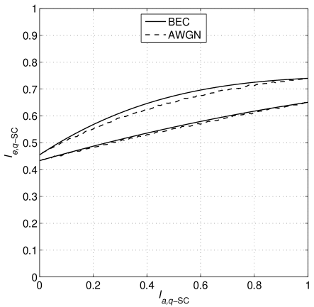
Figure 4: EXIT function for the $q$-SC front-end with BEC (analytical) and Gaussian (simulated) a priori messages for $\epsilon=0.25$, $m=4$ (lower curves) and $m=8$ (upper curves).

Since $\beta_{[i]}=0$ corresponds to $\epsilon_{i}=1/2$ through (-A), this case is equivalently described by an erasure. Therefore, the extrinsic messages can be modeled as being transmitted over a binary symmetric erasure channel (BSEC), with parameters $\epsilon_{m-t}$ and $\delta_{m-t}$ given by (2) and (3), respectively, since $t$ erasures correspond to the situation in layer $i=m-t$ in the layered scheme of Section II. Its capacity is thus

$$I_{t}=\left(1-\delta_{m-t}\right)\left(1-h\left(\frac{\epsilon_{m-t}}{1-\delta_{m-t}}\right)\right).$$ (16)

In order to compute the extrinsic information $I_{e}(I_{a})$ at the output of the front-end as

$$I_{e}(I_{a})=\sum_{t=0}^{m-1}I_{t}\lambda_{t}(I_{a}),$$ (17)

we have to compute the probability $\lambda_{t}(I_{a})$ that $t$ messages are erased given a priori mutual information $I_{a}$. Let $\Delta_{a}=1-I_{a}$ denote the probability that an a priori message is erased. The probability that $t=0,\ldots,m-1$ out of $m-1$ messages are erased is computed as

$$\lambda_{t}(I_{a}) =\binom{m-1}{t}\Delta_{a}^{t}\left(1-\Delta_{a}\right)^{m-1-t}$$

$$=\binom{m-1}{t}\left(1-I_{a}\right)^{t}I_{a}^{m-1-t}.$$ (18)

The EXIT function for BEC a priori messages can therefore be computed using (2), (3), (16) and (III-C) in (17).

Theorem 2

An iterative decoder for the bit-symmetric scheme using a $q$-SC front-end can attain $q$-SC capacity.

Proof:

According to the area theorem for EXIT charts [14], the capacity of each bit layer is given by the area below the EXIT function, if the a priori messages are modeled as coming from a BEC. Therefore, the capacity of the overall channel is given by

$$C_{\text{tot}} = m\int_{0}^{1}\sum_{t=0}^{m-1}I_{t}\lambda_{t}(I_{a})\,{\mathrm{d}}I_{a}$$ (19)

$$= m\sum_{t=0}^{m-1}I_{t}\int_{0}^{1}\lambda_{t}(I_{a})\,{\mathrm{d}}I_{a}$$

$$= m\sum_{t=0}^{m-1}I_{t}\binom{m-1}{t}\int_{0}^{1}\left(1-I_{a}\right)^{t}I_{a}^{m-1-t}\,{\mathrm{d}}I_{a}$$

$$= m\sum_{t=0}^{m-1}I_{t}\frac{(m-1)!}{(m-1-t)!t!}\frac{t!(m-1-t)!}{m!}$$

$$= \sum_{t=0}^{m-1}I_{t}=C_{\text{$q$-SC}},$$

where we used the fact that the integral corresponds to the definition of the beta function. The last sum in (19) is indeed equal to the capacity of the $q$-SC, as was already shown in the proof of Theorem 1. ∎

Without iterative processing, the maximum achievable rate is given by $I_{e}(0)$. In that case, all a priori messages are erased and one has

$$I_{m-1}=1-h\left(\epsilon_{1}\right)=1-h\left(\frac{pq}{2(q-1)}\right)=C_{\text{BSC}},$$

which corresponds to the simplistic coding approach where the $q$-SC is decomposed into $m$ BSCs.

Figure 4 shows an EXIT chart for BEC a priori messages. If the $q$-SC would be decomposed into BSCs (without iterating between the front-end and the LDPC code and without using the layered scheme) then the value at $I_{a}=0$ corresponds to the capacity of these BSCs. In contrast, the area below the EXIT functions corresponds to the normalized capacity of the $q$-SC. When using this front-end with an LDPC code, the a priori messages can not be modeled as coming from a BEC channel. For code design, we will make the approximation that the messages are Gaussian distributed, which is a common assumption when using EXIT charts. The simulated EXIT function using Gaussian a priori messages is also shown in Figure 4.

IV LDPC Design and Construction

After obtaining the EXIT function of the $q$-SC front-end, we can design an LDPC code. Code design is an optimization problem that selects the degree distributions of the code in order to maximize the rate, under the constraint that the EXIT function of the overall LDPC code does not intersect the EXIT function of the $q$-SC front-end.

Joint optimization of the variable and check node degree distributions is a nonlinear problem, but it was shown in [12] that the optimization of the check node degree distribution given a fixed variable node degree distribution is a linear programming problem, which can be solved efficiently.

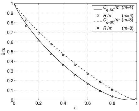
Figure 5: Rate of optimized codes versus normalized capacity of the $q$-SC for $m=4$ and $m=8$.

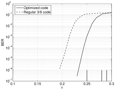
Figure 6: Bit error rate simulation for rate 1/2 LDPC decoding ($m=4$, $k=1500$ symbols). Marks indicate decoding threshold for regular code ($\epsilon=0.25$), optimized code ($\epsilon=0.28$) and Shannon limit ($\epsilon=0.29$).

To reduce the optimization complexity and to obtain practical degree distributions, we choose three non-zero variable node degrees (compare e.g., the approach in [15]). This allows to perform an exhaustive search over the variable node degree distribution, and for each variable node degree distribution we optimize the check node degree distribution as described in [12] with a maximum check node degree $d_{c,max}=50$.

Fig. 5 shows the normalized capacity of the $q$-SC and the obtained optimized code rates (under the Gaussian approximation) versus the error probability $\epsilon$ of the $q$-SC for $m=4$ and $m=8$. Using this code optimization, we are able to design codes that perform close to capacity over a wide range of error probabilities for moderate $q$.

For the actual code construction, we used a modified version of the PEG algorithm [16, 17], which allows us to construct codes with a specific variable and check node degree distribution. To avoid (short) cycles in the overall factor graph, one has to ensure that the bits of a given $q$-ary symbol do not participate in the same parity check. This can be achieved by using an appropriate interleaver between the $q$-SC front-end and the LDPC decoder. Another way would be to use the multi-edge type framework for LDPC code where such constraints can be explicitly specified [9, Chap. 7].

To verify our derivations, we performed bit error rate simulations for an optimized binary LDPC code of rate $R=1/2$ and length $N=12000$, shown in Fig. 6. This code is optimized for a $q$-SC with $m=4$, thus $N=12000$ bits correspond to $k=1500$ $q$-ary symbols. It has a decoding threshold of $\epsilon=0.28$ (the Shannon limit for $R=1/2$ is at $\epsilon=0.29$). As a comparison we also show the bit error rate for a regular LDPC code with $d_{v}=3$ and $d_{c}=6$ which has a decoding threshold of $\epsilon=0.25$.

V Generalization to Conditionally Independent Binary Sub-channels

The decoder in Section III is seen to easily extend to $q$-ary channels with modulo-additive noise, where the $m$ bits of the noise (error pattern) are independent if an error occurs, i.e. if at least one bit is nonzero. This assumption leads to define the $q$-ary symmetric channel with conditionally independent binary sub-channels ($q$-SC*), with transition probabilities

$$P_{Y|X}(y|x) =\begin{cases}1-\epsilon,&y=x,\\ \alpha\prod_{i=1}^{m}\epsilon_{i|*}^{x_{i}\oplus y_{i}}\left(1-\epsilon_{i|*}\right)^{1\oplus x_{i}\oplus y_{i}},&y\neq x,\end{cases}$$

$$\text{where}\quad\alpha =\frac{\epsilon}{1-\prod_{i=1}^{m}\left(1-\epsilon_{i|*}\right)}$$

and $\oplus$ denotes GF($2$) addition (this definition encompasses all channels satisfying the above conditional independence assumption, from which it may be derived axiomatically). The defining parameters are the symbol error probability $\epsilon$ and the $m$ conditional probabilities $\epsilon_{i|*}$, which are the bit error probabilities conditioned on the event that at least one of the other $m-1$ bits is in error. The marginal bit error probabilities will be $\epsilon_{i}=\alpha\epsilon_{i|*}$. Since the $q$-SC* is strongly symmetric, the uniform input distribution achieves its capacity

$$\hfill C_{\text{$q$-SC*}}=m-\alpha\sum_{i=1}^{m}h(\epsilon_{i|*})+(1-\epsilon)\log_{2}(1-\epsilon)+\alpha\log_{2}\alpha-(\alpha-\epsilon)\log_{2}(\alpha-\epsilon).\hfill$$

When $\epsilon$ is such that $\alpha=1$, the $q$-SC* reduces to $m$ independent BSCs, while for $\epsilon_{i|*}=\frac{1}{2}$, $i=1,\ldots,m$, it becomes an ordinary $q$-SC.

$$L_{\mathrm{app}}(X^{j}_{i}\!=\!y^{j}_{i}) =\log\left(\frac{(1-\epsilon)\beta^{j}+\alpha(1-\epsilon_{i|*})p^{j}_{i}\left[\prod_{k\neq i}\left(\epsilon_{k|*}+p^{j}_{k}-2\epsilon_{k|*}p^{j}_{k}\right)-\prod_{k\neq i}(1-\epsilon_{k|*})p^{j}_{k}\right]}{\alpha\epsilon_{i|*}(1-p^{j}_{i})\prod_{k\neq i}\left(\epsilon_{k|*}+p^{j}_{k}-2\epsilon_{k|*}p^{j}_{k}\right)}\right)$$

$$=\log\left(\frac{(1-\alpha)\beta^{j}_{[i]}+\alpha(1-\epsilon_{i|*})\prod_{k\neq i}\left(\epsilon_{k|*}+p^{j}_{k}-2\epsilon_{k|*}p^{j}_{k}\right)}{\alpha\epsilon_{i|*}\prod_{k\neq i}\left(\epsilon_{k|*}+p^{j}_{k}-2\epsilon_{k|*}p^{j}_{k}\right)}\right)+\log\left(\frac{p^{j}_{i}}{1-p^{j}_{i}}\right)$$

$$=\underbrace{\log\left(\frac{1-\epsilon_{i|*}}{\epsilon_{i|*}}+\frac{(1-\alpha)\beta^{j}_{[i]}}{\alpha\epsilon_{i|*}\prod_{k\neq i}\left(\epsilon_{k|*}+p^{j}_{k}-2\epsilon_{k|*}p^{j}_{k}\right)}\right)}_{\text{\normalsize$L_{\text{ch}}(X^{j}_{i}\!=\!y^{j}_{i})$}}+L_{\mathrm{extr}}(X^{j}_{i}\!=\!y^{j}_{i}).$$ (20)

The unnormalized bit APP (compare (12)) is obtained as

$$P(X^{j}_{i}=x^{j}_{i}|\mathbf{Y}=\mathbf{y})\doteq\begin{cases}(1-\epsilon)\prod_{k=1}^{m}p^{j}_{k}\\ \quad+\alpha(1-\epsilon_{i|*})p^{j}_{i}\Big{[}\prod_{k\neq i}\big{(}\epsilon_{k|*}+p^{j}_{k}-2\epsilon_{k|*}p^{j}_{k}\big{)}-\prod_{k\neq i}(1-\epsilon_{k|*})p^{j}_{k}\Big{]},\quad x^{j}_{i}=y^{j}_{i},\\ \alpha\epsilon_{i|*}(1-p^{j}_{i})\prod_{k\neq i}\big{(}\epsilon_{k|*}+p^{j}_{k}-2\epsilon_{k|*}p^{j}_{k}\big{)},\hfill x^{j}_{i}\neq y^{j}_{i},\end{cases}$$

leading to the LLR expression (V). The quantities $p^{j}_{i}$, $\beta^{j}$ and $\beta^{j}_{[i]}$ are as defined in Section III. Like in the special case of the $q$-SC, for $\beta^{j}_{[i]}\to 0$ the channel LLR $L_{\text{ch}}$ tends to a constant, which is equal to the LLR of the binary sub-channel conditioned on the occurrence of an error on one or more of the other sub-channels. The initial value of $L_{\text{ch}}$ can again be obtained by assuming a worst-case of $p^{j}_{k}=\frac{1}{2}$, $\beta^{j}_{[i]}=2^{-m+1}$ in (V), yielding

$$L_{\text{ch}}^{(0)}(X^{j}_{i}\!=\!y^{j}_{i}) =\log\left(\frac{1-\epsilon_{i|*}}{\epsilon_{i|*}}+\frac{1-\alpha}{\alpha\epsilon_{i|*}}\right)$$

$$=\log\left(\frac{1-\alpha\epsilon_{i|*}}{\alpha\epsilon_{i|*}}\right)=\log\left(\frac{1-\epsilon_{i}}{\epsilon_{i}}\right),$$

which is the channel LLR of the marginal BSC.

-A Simplification of the Messages

Since all involved variables are binary, we can represent the messages by scalar quantities. For the messages from and to the variable nodes $x^{j}_{i}$ of the LDPC code, we use log-likelihood ratios of the corresponding messages

$$L_{a,i}=\log\frac{\mu_{x_{i}\to f_{\text{ch}}}(0)}{\mu_{x_{i}\to f_{\text{ch}}}(1)},$$

$$L_{\text{ch},i}=\log\frac{\mu_{f_{\text{ch}}\to x_{i}}(0)}{\mu_{f_{\text{ch}}\to x_{i}}(1)}.$$

The messages from the function nodes $f_{\text{ch}}$ to the node $f_{E}$ are defined as the probability of no error

$$p_{i}=\mu_{f_{\text{ch}}\to e_{i}}(0)=\mu_{e_{i}\to f_{E}}(0),$$

and the messages from the function node $f_{E}$ are defined as the error probability

$$\epsilon_{i}=\frac{\mu_{f_{E}\to e_{i}}(1)}{\mu_{f_{E}\to e_{i}}(0)+\mu_{f_{E}\to e_{i}}(1)}.$$

Using these definitions, we can reformulate the computation rules at the function nodes as

$$p_{i}=\frac{e^{\frac{L_{a,i}}{2}\cdot(1-2y_{i})}}{e^{\frac{L_{a,i}}{2}}+e^{-\frac{L_{a,i}}{2}}},$$

and

$$\epsilon_{i} =\frac{\frac{\epsilon}{q-1}}{(1-\epsilon)\cdot\beta_{[i]}+\frac{\epsilon}{q-1}\left(1-\beta_{[i]}\right)+\frac{\epsilon}{q-1}}$$

$$=\frac{\epsilon}{2\epsilon+\beta_{[i]}(q-\epsilon q-1)}$$ (21)

For the initialization, we set all a-priori L-values $L_{a,i}$ to zero, leading to $\beta_{[i]}=2^{-(m-1)}=2/q$. Inserting this in (-A) leads to

$$\epsilon_{i}=\frac{\epsilon q}{2(q-1)}=\epsilon_{\text{BSC}}.$$

Finally, the messages sent from the function nodes $f_{\text{ch}}$ to the variable nodes $x_{i}$ are computed as

$$L_{\text{ch},i}=(1-2y_{i})\cdot\log\frac{1-\epsilon_{i}}{\epsilon_{i}}.$$

References

- [1] M. G. Luby and M. Mitzenmacher, “Verification-based decoding for packet-based low-density parity-check codes,” IEEE Trans. Inform. Theory, vol. 51, no. 1, pp. 120–127, Jan. 2005.
- [2] A. Brown, L. Minder, and A. Shokrollahi, “Probabilistic decoding of interleaved RS-codes on the -ary symmetric channel,” in Proc. IEEE Int. Symp. Information Theory (ISIT), Chicago, USA, Jun. 27 – Jul. 2, 2004.
- [3] A. Shokrollahi and W. Wang, “Low-density parity-check codes with rates very close to the capacity of the -ary symmetric channel for large ,” in Proc. IEEE Int. Symp. Information Theory (ISIT), Chicago, USA, Jun. 27 – Jul. 2, 2004.
- [4] A. Shokrollahi, “Capacity-approaching codes on the -ary symmetric channel for large ,” in Proc. ITW, San Antonio, Texas, USA, Oct. 24 – 29, 2004.
- [5] F. Zhang and H. D. Pfister, “Analysis of verification-based decoding on the -ary symmetric channel for large ,” IEEE Trans. Inform. Theory, vol. 57, no. 10, pp. 6754–6770, Oct. 2011. [Online]. Available: http://arxiv.org/abs/0806.3243
- [6] C. Weidmann, F. Bassi, and M. Kieffer, “Practical distributed source coding with impulse-noise degraded side information at the decoder,” in Proc. EUSIPCO, Lausanne, Switzerland, Aug. 2008.
- [7] M. C. Davey and D. MacKay, “Low density parity check codes over GF(),” IEEE Commun. Lett., vol. 2, pp. 165–167, Jun. 1998.
- [8] D. Declercq and M. Fossorier, “Decoding algorithms for nonbinary LDPC codes over GF(),” IEEE Trans. Commun., vol. 55, no. 4, pp. 633–643, Apr. 2007.
- [9] T. Richardson and R. Urbanke, Modern Coding Theory. Cambridge University Press, 2008, see also http://lthcwww.epfl.ch/mct/index.php.
- [10] S. ten Brink, G. Kramer, and A. Ashikhmin, “Design of low-density parity-check codes for modulation and detection,” IEEE Trans. Commun., vol. 52, no. 4, pp. 670–678, Apr. 2004.
- [11] A. Sanderovich, M. Peleg, and S. Shamai, “LDPC coded MIMO multiple access with iterative joint decoding,” IEEE Trans. Inform. Theory, vol. 51, no. 4, pp. 1437–1450, Apr. 2005.
- [12] G. Lechner, J. Sayir, and I. Land, “Optimization of LDPC codes for receiver frontends,” in Proc. IEEE Int. Symp. Information Theory (ISIT), Seattle WA, USA, Jul. 9–14, 2006.
- [13] F. Kschischang, B. Frey, and H.-A. Loeliger, “Factor graphs and the sum-product algorithm,” IEEE Trans. Inform. Theory, vol. 47, no. 2, pp. 498–519, Feb. 2001.
- [14] A. Ashikhmin, G. Kramer, and S. ten Brink, “Extrinsic information transfer functions: Model and erasure channel properties,” IEEE Trans. Inform. Theory, vol. 50, no. 11, pp. 2657–2673, Nov. 2004.
- [15] S. ten Brink and G. Kramer, “Design of repeat-accumulate codes for iterative detection and decoding,” IEEE Trans. Signal Proc., vol. 51, no. 11, pp. 2764–2772, Nov. 2003.
- [16] X.-Y. Hu, E. Eleftheriou, and D. Arnold, “Regular and irregular progressive edge-growth Tanner graphs,” IEEE Trans. Inform. Theory, vol. 51, no. 1, pp. 386–398, Jan. 2005.
- [17] X.-Y. Hu, “Software for PEG code construction.” [Online]. Available: http://www.inference.phy.cam.ac.uk