The $N_{\rm f}^{3}g^{6}$ term in the pressure of hot QCD

Abstract

We determine the first independent part of the $g^{6}$ coefficient in the weak coupling expansion of the QCD pressure at high temperatures, the one proportional to the maximal power of the number of quark flavors $N_{\rm f}$. In addition to introducing and developing computational methods that can be used in evaluating other parts of the expansion, our calculation provides a result that becomes dominant in the limit of large $N_{\rm f}$ and a fixed effective coupling $g_{\mathrm{eff}}^{2}\equiv g^{2}N_{\rm f}/2$.

I Introduction

The single most fundamental quantity characterizing the bulk properties of a system in thermodynamic equilibrium is its partition function, or equivalently the functional dependence of its pressure $p$ on the temperature $T$ (and other parameters such as the chemical potentials). In the case of hot quantum chromodynamics (QCD), this function has been extensively studied both on the lattice Aoki et al. (2006); Cheng et al. (2008) and using perturbation theory, with the purpose of obtaining a consistent description of the quantity all the way from the phase transition region ($T\sim T_{c}$) to asymptotically high temperatures. At present, the state of the art on the perturbative (high $T$) side is order $g^{6}\ln\,g$ in the strong coupling constant, which has been reached both at zero and finite quark chemical potentials Kajantie et al. (2003a); Vuorinen (2003). In addition, perturbative methods have been successfully applied to a plethora of other quantities (for some recent results, see e.g. Refs. Chesler et al. (2009); Laine and Schroder (2005); Carrington et al. (2008) and references therein).

A persistent problem in perturbative finite temperature QCD is the slow convergence of the various weak coupling expansions. For most quantities, the issue can be traced back to the contributions of the soft ($gT$) and ultrasoft ($g^{2}T$) energy scales, which respectively enter through the three-dimensional effective theories EQCD and MQCD Braaten and Nieto (1996). In the case of the pressure, the contributions of these scales to the ${\mathcal{O}}(g^{6})$ term in the expansion have by now been determined Kajantie et al. (2003b); Di Renzo et al. (2006); Hietanen et al. (2005); Hietanen and Kurkela (2006), and to this end, there is clear motivation for evaluating the part corresponding to the hard ($2\pi T$) scales as well Laine (2003). This requires the evaluation of all four-loop vacuum diagrams in the full four-dimensional theory, a task that has already been completed in the similar, though technically much simpler, case of scalar $\phi^{4}$ theory Gynther et al. (2007); Andersen et al. (2009).

The ${\mathcal{O}}(g^{6})$ contribution of the QCD pressure can be divided into several gauge invariant parts, proportional to various group theory invariants, most importantly powers of the number of fundamental fermion flavors $N_{\rm f}$. In the present paper, our purpose is to evaluate the first — and computationally most straightforward — of these, the one proportional to the maximal power $N_{\rm f}^{3}$. Our motivation for this is twofold. On one hand, we wish to demonstrate that the computational machinery built for three-loop QCD and four-loop $\phi^{4}$ theory calculations in Refs. Arnold and Zhai (1994, 1995); Gynther et al. (2007) can be straightforwardly applied to the four-loop level of QCD as well. In addition, the $N_{\rm f}^{3}$ term not only represents the first independent piece of the ${\mathcal{O}}(g^{6})$ coefficient, but in fact becomes dominant over all the other contributions in the limit of a large flavor number, where the effective coupling $g_{\mathrm{eff}}^{2}\equiv T_{F}g^{2}=N_{\rm f}g^{2}/2$ is kept fixed while $N_{\rm f}$ is taken to infinity. In this limit, the theory in fact somewhat trivializes, enabling an all orders numerical evaluation of the partition function Moore (2002); Ipp et al. (2003); Ipp and Rebhan (2003) and providing a rough numerical check for our result.

The paper is organized as follows. In the rest of the first Section, we present our notation and explain, how renormalization is performed in our work. After this, we proceed to review the organization of our calculation in Section II, while the bulk of the detailed computations is left to Section III. Our result is finally assembled and discussed in Section IV, where we in addition analyze the convergence of the weak coupling expansion of the pressure and draw our final conclusions.

I.1 Notation

We work in $d=4-2\epsilon$ dimensional Euclidean spacetime, using dimensional regularization to regulate both ultraviolet (UV) and infrared (IR) divergences. We use lower case bold letters to denote three-dimensional spatial vectors and capital letters for four-dimensional spacetime vectors $P=(p_{0},\bm{p})$, so that $P^{2}=P_{\mu}P_{\mu},\,p^{2}=p_{i}p_{i}$. As usual, sum-integrals are defined by

$$\int_{p}\equiv\Lambda^{2\epsilon}\int\frac{\mathrm{d}^{d-1}p}{(2\pi)^{d-1}}=\left(\frac{e^{\gamma_{\rm E}}\bar{\Lambda}^{2}}{4\pi}\right)\int\frac{\mathrm{d}^{d-1}p}{(2\pi)^{d-1}},$$ (1)

$$\hbox{$\sum$}\!\!\!\!\!\!\!\int_{P/\{P\}}\equiv T\sum_{p_{0}}\int_{p},\quad\hbox{$\sum{}^{\prime}$}\!\!\!\!\!\!\!\!\!\!\int_{P/\{P\}}\,\equiv\,T\sum_{p_{0}\neq 0}\int_{p},$$ (2)

where $\Lambda$ is the MS renormalization scale and $\bar{\Lambda}$ the $\overline{\mathrm{MS}}$ one, and $P/\{P\}$ refer to bosonic/fermionic Matsubara modes, respectively. Bosonic sum-integrals, in which the $p_{0}=0$ term has been subtracted out, are marked with a prime, and, borrowing notation from Refs. Arnold and Zhai (1994); Braaten and Nieto (1996), some standard sum-integrals are denoted by

$$\mathcal{I}_{n}^{m} \equiv \hbox{$\sum$}\!\!\!\!\!\!\!\int_{P}\frac{(p_{0})^{m}}{(P^{2})^{n}},$$ (3)

$$\widetilde{\mathcal{I}}_{n}^{m} \equiv \hbox{$\sum$}\!\!\!\!\!\!\!\int_{\{P\}}\frac{(p_{0})^{m}}{(P^{2})^{n}},$$ (4)

$$\Pi(P) \equiv \hbox{$\sum$}\!\!\!\!\!\!\!\int_{Q}\frac{1}{Q^{2}(Q-P)^{2}},$$ (5)

$$\Pi_{f}(P) \equiv \hbox{$\sum$}\!\!\!\!\!\!\!\int_{\{Q\}}\frac{1}{Q^{2}(Q-P)^{2}}.$$ (6)

We perform renormalization by consistently using the bare coupling $g_{B}$ in all of our calculations, and only in the end expressing the result in terms of the physical, renormalized one via the relation $g_{B}^{2}~{}=~{}Z_{g}g^{2}$. We need the parameter $Z_{g}$ to two-loop order, to which it reads

$$Z_{g} = 1+\frac{g^{2}}{(4\pi)^{2}}\frac{\beta_{1}}{\epsilon}+\frac{g^{4}}{(4\pi)^{4}}\left(\frac{\beta_{2}}{\epsilon^{2}}+\frac{\beta_{2}^{\prime}}{\epsilon}\right)+\dots$$ (7)

Here, the coefficients $\beta_{i}$ can for our purposes be deduced from the known exact beta-function of $N_{\rm f}\rightarrow\infty$ QCD,

$$\mu\frac{\partial g^{2}}{\partial\mu} = \frac{T_{F}g^{4}}{6\pi^{2}},\;\;\;T_{F}\equiv\frac{N_{\rm f}}{2},$$ (8)

giving us

$$\beta_{1} = \frac{4T_{F}}{3},\quad\beta_{2}\,=\,\beta_{1}^{2},\quad\beta_{2}^{\prime}\,=\,0.$$ (9)

In this limit, the running coupling correspondingly reads

$$\frac{1}{g^{2}(\bar{\Lambda})} = \frac{1}{g^{2}(\mu)}\left(1-\frac{T_{F}g^{2}(\mu)}{6\pi^{2}}\ln\frac{\bar{\Lambda}}{\mu}\right),$$ (10)

which this time is exact to all loop orders. It exhibits the well-known Landau singularity, which implies that large-$N_{f}$ QCD is well-defined only below some energy scale $\Lambda_{L}$.

Finally, in the course of our calculation, we will often switch to dimensionless integration variables without explicitly saying so. In all of these cases, the integration momenta and coordinates have been scaled by the appropriate power of $2\pi T$.

II Organizing the calculation

The weak coupling expansion of the QCD pressure is known to order $g^{6}\ln g$ for an arbitrary number of colors and massless fundamental fermion flavors Kajantie et al. (2003a); Vuorinen (2003). In the $N_{\rm f}\rightarrow\infty$ limit (with fixed $g_{\mathrm{eff}}^{2}$) and at zero chemical potential, the result reads Zhai and Kastening (1995)

$$\frac{p-p_{0}}{d_{A}} = \frac{\pi^{2}T^{4}}{45}\left[-\frac{g_{\mathrm{eff}}^{2}}{(4\pi)^{2}}\frac{25}{2}+\frac{g_{\mathrm{eff}}^{3}}{(4\pi)^{3}}\frac{80}{\sqrt{3}}+\frac{g_{\mathrm{eff}}^{4}}{(4\pi)^{4}}\left(\frac{100}{3}\ln\frac{\bar{\Lambda}}{4\pi T}+\frac{5}{3}-88\ln 2+20\gamma_{\rm E}+\frac{80}{3}\frac{\zeta^{\prime}(-1)}{\zeta(-1)}-\frac{40}{3}\frac{\zeta^{\prime}(-3)}{\zeta(-3)}\right)\right.$$ (11)

$$\hskip 31.2982pt\left.-\frac{g_{\mathrm{eff}}^{5}}{(4\pi)^{5}}\frac{320}{\sqrt{3}}\left(\ln\frac{\bar{\Lambda}}{4\pi T}-\frac{1}{2}+2\ln 2+\gamma_{\rm E}\right)+\frac{g_{\mathrm{eff}}^{6}}{(4\pi)^{6}}p_{6}+\mathcal{O}(g^{7})\right],$$

in which we wish to compute the unknown coefficient $p_{6}$ that is nothing but the $N_{f}^{3}g^{6}$ term in the full theory pressure. Here, we have subtracted out the pressure of a gas of free quarks and gluons, $p_{0}=\pi^{2}T^{4}/45\,(d_{A}+7N_{\rm c}N_{\rm f}/4)$, where $d_{A}\equiv N_{\rm c}^{2}-1$ and which dominates the pressure in the large $N_{\rm f}$ limit (for all $g_{\mathrm{eff}}^{2}$).

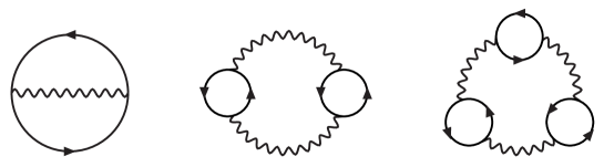
Figure 1: The two-, three- and four-loop Feynman diagrams contributing to $p_{\rm E}$ in the large $N_{\rm f}$ limit. The straight lines with an arrow correspond to quarks, and the wavy lines to gluons.

At leading order in the large $N_{\rm f}$ expansion of $p-p_{0}$, the effective three-dimensional theories EQCD and MQCD, which incorporate the effects of the soft scales $gT$ and $g^{2}T$ to the pressure, do not contribute to the coefficients of even powers of $g$. We can thus concentrate on evaluating the contribution of the hard scale, corresponding to the strict (unresummed) perturbation expansion of the pressure in the four-dimensional theory, commonly denoted by $p_{\rm E}$. We note that while this function suffers from IR divergences that for finite $N_{\rm f}$ are canceled by UV divergences in the effective theory contributions, in the large $N_{\rm f}$ limit they are all guaranteed to vanish in dimensional regularization.

In the large $N_{\rm f}$ limit, the function $p_{\rm E}$ has a simple diagrammatic expansion of the form

$$\frac{p_{\rm E}}{d_{A}} = \frac{1}{2}Z_{g}g^{2}I_{a}+\frac{1}{4}Z_{g}^{2}g^{4}I_{b}+\frac{1}{6}Z_{g}^{3}g^{6}I_{c}+\dots,$$ (12)

where we have denoted

$$I_{a} = -\hbox{$\sum$}\!\!\!\!\!\!\!\int_{P}\frac{\Pi_{\mu\mu}}{P^{2}},$$ (13)

$$I_{b} = \hbox{$\sum$}\!\!\!\!\!\!\!\int_{P}\frac{\Pi_{\mu\nu}\Pi_{\nu\mu}}{P^{4}},$$ (14)

$$I_{c} = -\hbox{$\sum$}\!\!\!\!\!\!\!\int_{P}\frac{\Pi_{\mu\nu}\Pi_{\nu\rho}\Pi_{\rho\mu}}{P^{6}},$$ (15)

and the integrals correspond to the three Feynman graphs in Fig. 1. Here, the one-loop large $N_{\rm f}$ gluon self energy reads

$$\Pi_{\mu\nu}(P) = -2T_{F}\left[2\widetilde{\mathcal{I}}_{1}^{0}\delta_{\mu\nu}-(\delta_{\mu\nu}P^{2}-P_{\mu}P_{\nu})\Pi_{f}(P)\right.$$ (16)

$$\hskip 28.45274pt\left.-\hbox{$\sum$}\!\!\!\!\!\!\!\int_{\{Q\}}\frac{(2Q-P)_{\mu}(2Q-P)_{\nu}}{Q^{2}(Q-P)^{2}}\right],$$

in which the color indices have been suppressed (the trace over them having already been carried out).

At this point, we may simplify the calculations by dividing the self energy into its three-dimensionally longitudinal and transverse components (for a precise definition, see e.g. Ref. Kapusta and Gale (2006)), in terms of which the above integrals read

$$I_{a} = -\hbox{$\sum$}\!\!\!\!\!\!\!\int_{P}\frac{\Pi_{L}(P)+(d-2)\Pi_{T}(P)}{P^{2}},$$ (17)

$$I_{b} = \hbox{$\sum$}\!\!\!\!\!\!\!\int_{P}\frac{\Pi_{L}(P)^{2}+(d-2)\Pi_{T}(P)^{2}}{P^{4}},$$ (18)

$$I_{c} = -\hbox{$\sum$}\!\!\!\!\!\!\!\int_{P}\frac{\Pi_{L}(P)^{3}+(d-2)\Pi_{T}(P)^{3}}{P^{6}}.$$ (19)

Extracting now the UV divergences of the self-energies by denoting

$$\Pi_{L/T}(P) \equiv \overline{\Pi}_{L/T}(P)+\frac{\beta_{1}}{(4\pi)^{2}}\frac{P^{2}}{\epsilon},$$ (20)

the expression for the function $p_{\rm E}$ up to order $g^{6}$ obtains the remarkably simple form

$$\frac{p_{\rm E}}{d_{A}} = \frac{1}{2}g^{2}I_{a}+\frac{1}{4}g^{4}\overline{I}_{b}+\frac{1}{6}g^{6}\overline{I}_{c}.$$ (21)

Here, the bars in $\overline{I}_{b,c}$ denote the replacing of $\Pi_{L/T}(P)$ by $\overline{\Pi}_{L/T}(P)$ (note that with this definition $I_{a}=\overline{I}_{a}$), and Eq. (9) has been used to cancel terms originating from the renormalization corrections against those left over from the redefinition of Eq. (20). As $I_{a}$ and $\overline{I}_{b}$ are both known, we are only left with the task of computing $\overline{I}_{c}$, which is furthermore observed to be finite in dimensional regularization.

For notational simplicity, it is convenient to separate the $T=0$ contributions of the self-energies by writing

$$\overline{\Pi}_{L/T}(P) = \overline{\Pi}_{L/T}^{(0)}(P)+\overline{\Pi}_{L/T}^{(T)}(P).$$ (22)

We find that, in various limits, the two parts of the functions can be written as:

• at $T=0$:

  $$\overline{\Pi}_{L/T}^{(0)}(P) = \frac{4T_{F}}{3}\frac{P^{2}}{(4\pi)^{2}}\left[A(\epsilon)\left(\frac{\Lambda^{2}}{P^{2}}\right)^{\epsilon}-\frac{1}{\epsilon}\right]$$

  $$= \frac{4T_{F}}{3}\frac{P^{2}}{(4\pi)^{2}}\left(\frac{5}{3}+\ln\frac{\bar{\Lambda}^{2}}{P^{2}}+\mathcal{O}(\epsilon)\right),$$

  $$\equiv \overline{\Pi}^{(0)}(P),$$

  $$A(\epsilon) = \frac{6(4\pi)^{\epsilon}\Gamma(\epsilon)\Gamma(2-\epsilon)^{2}}{\Gamma(4-2\epsilon)},$$

• at $\epsilon=0$:

  $$\overline{\Pi}_{L}^{(T)}(P) = 2T_{F}\left(\frac{T^{2}}{6}\delta_{p_{0}}+\frac{P^{2}}{32\pi^{3}}R^{+}(n,\tilde{p})\right),$$ (24)

  $$\overline{\Pi}_{T}^{(T)}(P) = T_{F}\frac{P^{2}}{32\pi^{3}}R^{-}(n,\tilde{p}),$$ (25)

  $$R^{\pm}(n,\tilde{p}) = \int\frac{d^{3}r}{r^{2}}\left(1\pm\frac{1}{r^{2}}\partial^{2}_{\tilde{p}}\right)\mathrm{e}^{i\tilde{\bm{p}}\cdot\bm{r}}\mathrm{e}^{-|n|r}$$

  $$\times\left(\mathrm{csch}\,r-\frac{1}{r}+\frac{r}{6}(1-\delta_{n,0})\right),$$

  $$\mathrm{where}\,(n,\,\tilde{\bm{p}}) = (p_{0}/(2\pi T),\,\bm{p}/(2\pi T)),$$

• at $P\rightarrow\infty$ (up to but not including order $T^{6}/P^{4}$):

  $$\overline{\Pi}_{L}^{(T)}(P) = 16T_{F}\frac{d-2}{d-1}\frac{T^{4}}{P^{2}}B(\epsilon),$$ (26)

  $$\overline{\Pi}_{T}^{(T)}(P) = 16T_{F}\frac{1}{d-1}\frac{dp_{0}^{2}-2P^{2}}{P^{4}}T^{4}\,B(\epsilon),$$ (27)

  $$B(\epsilon) = \frac{1-2^{2\epsilon-3}}{4\pi^{3/2}}\frac{\Gamma(4-2\epsilon)\zeta(4-2\epsilon)}{\Gamma(3/2-\epsilon)}\left(\frac{4\pi\Lambda^{2}}{T^{2}}\right)^{\epsilon},$$

• at $p\rightarrow 0$ (up to but not including order $p^{4}$):

  $$\overline{\Pi}_{L}^{(T)}(p_{0}=0,p) = \frac{4T_{F}}{3}\left\{-3(d-2)\widetilde{\mathcal{I}}_{1}^{\,0}\right.$$

  $$\left.+\left[\frac{d-2}{2}\widetilde{\mathcal{I}}_{2}^{\,0}-\frac{A(\epsilon)}{(4\pi)^{2}}\left(\frac{\Lambda^{2}}{p^{2}}\right)^{\epsilon}\right]p^{2}\right\},$$

  $$\overline{\Pi}_{T}^{(T)}(p_{0}=0,p) = \frac{4T_{F}}{3}\left[\widetilde{\mathcal{I}}_{2}^{\,0}-\frac{A(\epsilon)}{(4\pi)^{2}}\left(\frac{\Lambda^{2}}{p^{2}}\right)^{\epsilon}\right]p^{2}.$$ (29)

The required integral can then be divided into four parts,

$$-\overline{I}_{c} = \hbox{$\sum$}\!\!\!\!\!\!\!\int_{P}\frac{\overline{\Pi}_{L}(P)^{3}+(d-2)\overline{\Pi}_{T}(P)^{3}}{P^{6}}$$ (30)

$$= \hbox{$\sum$}\!\!\!\!\!\!\!\int_{P}\frac{(d-1)\overline{\Pi}^{(0)}(P)^{3}}{P^{6}}$$

$$+ 3\,\hbox{$\sum$}\!\!\!\!\!\!\!\int_{P}\frac{\overline{\Pi}_{L}^{(T)}(P)+(d-2)\overline{\Pi}_{T}^{(T)}(P)}{P^{6}}\overline{\Pi}^{(0)}(P)^{2}$$

$$+ 3\,\hbox{$\sum$}\!\!\!\!\!\!\!\int_{P}\frac{\overline{\Pi}_{L}^{(T)}(P)^{2}+(d-2)\overline{\Pi}_{T}^{(T)}(P)^{2}}{P^{6}}\overline{\Pi}^{(0)}(P)$$

$$+ \hbox{$\sum$}\!\!\!\!\!\!\!\int_{P}\frac{\overline{\Pi}_{L}^{(T)}(P)^{3}+(d-2)\overline{\Pi}_{T}^{(T)}(P)^{3}}{P^{6}}$$

$$\equiv K_{1}+3K_{2}+3K_{3}+K_{4}.$$

Of these terms, $K_{1}$ and $K_{2}$ are UV divergent but IR finite, while $K_{3}$ and $K_{4}$ are UV finite but IR divergent. In the following Section, we will set out to evaluate these functions one by one.

III Evaluation of the integrals

In performing the integrals $K_{1}$–$K_{4}$, we employ the general strategy of first identifying their UV and IR divergent parts, and then separating them from the rest, writing

$$K_{i} = K_{i}^{\mathrm{div}}+K_{i}^{\mathrm{fin}}.$$ (31)

The divergent pieces must be evaluated analytically in $d=4-2\epsilon$ dimensions, whereas in the finite integrals we may set $d=4$ and use the integral representations of Eqs. (24) and (25) for the self-energies. Apart from the case of $K_{4}$, which is treated separately, the subtracted divergent pieces are always identified with specific parts of the integrands of Eqs. (24) and (25), corresponding to terms in the Taylor expansion of the hyperbolic cosecant.

For ease of notation, we write the finite parts of the $K_{i}$ in terms of dimensionless integrals $M_{i}$,

$$K_{i}^{\mathrm{fin}} = \frac{16T_{F}^{3}}{9}\frac{T^{4}}{(4\pi)^{4}}M_{i},$$ (32)

which one can, when necessary, easily evaluate with numerical tools.

III.1 $K_{1}$ integral

Using the expression of Eq. (• ‣ II) for $\overline{\Pi}^{(0)}(P)$, the integral $K_{1}$ can be trivially expressed in terms of the $\mathcal{I}^{m}_{n}$ functions,

$$K_{1} = \frac{T_{F}^{3}}{1728\pi^{6}}(d-1)\left[A(\epsilon)^{3}\Lambda^{6\epsilon}\mathcal{I}_{3\epsilon}^{0}-\frac{3}{\epsilon}A(\epsilon)^{2}\Lambda^{4\epsilon}\mathcal{I}_{2\epsilon}^{0}\right.$$ (33)

$$\left.\hskip 71.13188pt+\frac{3}{\epsilon^{2}}A(\epsilon)\Lambda^{2\epsilon}\mathcal{I}_{\epsilon}^{0}\right].$$

The values of all of the integrals appearing here are available in the literature (see e.g. Ref. Arnold and Zhai (1994)), giving in the end

$$K_{1} = \frac{T_{F}^{3}T^{4}}{135(2\pi)^{4}}\Bigg{\{}\bigg{(}\ln\frac{\bar{\Lambda}}{4\pi T}\bigg{)}^{2}+\Big{(}\frac{13}{3}+2\frac{\zeta^{\prime}(-3)}{\zeta(-3)}\Big{)}\ln\frac{\bar{\Lambda}}{4\pi T}$$ (34)

$$+ \frac{209}{36}+\frac{\pi^{2}}{12}+\frac{13}{3}\frac{\zeta^{\prime}(-3)}{\zeta(-3)}+\frac{\zeta^{\prime\prime}(-3)}{\zeta(-3)}\Bigg{\}}.$$

III.2 $K_{2}$ integral

The $K_{2}$ integral is logarithmically UV divergent due to the integrand behaving like $1/P^{4}$ at large $P$. Separating thus its large $P$ limit from the rest, we easily find for the divergent part

$$K_{2}^{\mathrm{div}} = 16T_{F}\frac{d-2}{d-1}B(\epsilon)\hbox{$\sum$}\!\!\!\!\!\!\!\int_{P}\frac{dp_{0}^{2}-P^{2}}{P^{10}}\overline{\Pi}^{(0)}(P)^{2}$$ (35)

$$= \frac{T_{F}^{3}}{9\pi^{4}}\frac{d-2}{d-1}B(\epsilon)$$

$$\times \!\!\left[d\left(A(\epsilon)^{2}\Lambda^{4\epsilon}\mathcal{I}_{3+2\epsilon}^{2}-\frac{2}{\epsilon}A(\epsilon)\Lambda^{2\epsilon}\mathcal{I}_{3+\epsilon}^{2}+\frac{1}{\epsilon^{2}}\mathcal{I}_{3}^{2}\right)\right.$$

$$\left.\!\!-\left(A(\epsilon)^{2}\Lambda^{4\epsilon}\mathcal{I}_{2+2\epsilon}^{0}-\frac{2}{\epsilon}A(\epsilon)\Lambda^{2\epsilon}\mathcal{I}_{2+\epsilon}^{0}+\frac{1}{\epsilon^{2}}\mathcal{I}_{2}^{0}\right)\right],$$

where all terms are again readily available.

The finite part of the integral is most conveniently evaluated in two pieces. Starting from the $p_{0}\neq 0$ terms, we obtain using the notation of Eq. (32)

$$M_{2}^{\prime} = 2\sum_{n=1}^{\infty}\int\frac{d^{3}p}{(2\pi)^{3}}\left(\frac{5}{3}+\ln\frac{\bar{\Lambda}^{2}}{4\pi^{2}T^{2}}-\ln(n^{2}+p^{2})\right)^{2}$$ (37)

$$\times\int\frac{d^{3}r}{r^{2}}\mathrm{e}^{i\bm{p}\cdot\bm{r}}\mathrm{e}^{-nr}\left(\mathrm{csch}\,r-\frac{1}{r}+\frac{r}{6}-\frac{7r^{3}}{360}\right)$$

$$\equiv \left(\frac{5}{3}+\ln\frac{\bar{\Lambda}^{2}}{4\pi^{2}T^{2}}\right)^{2}M_{2}^{\prime}{}^{0}$$

$$-2\left(\frac{5}{3}+\ln\frac{\bar{\Lambda}^{2}}{4\pi^{2}T^{2}}\right)M_{2}^{\prime}{}^{1}+M_{2}^{\prime}{}^{2},$$

where we have defined

$$M_{2}^{\prime}{}^{k} \equiv 2\sum_{n=1}^{\infty}\int\frac{d^{3}p}{(2\pi)^{3}}\int\frac{d^{3}r}{r^{2}}\left[\ln(n^{2}+p^{2})\right]^{k}\,\mathrm{e}^{i\bm{p}\cdot\bm{r}}\mathrm{e}^{-nr}$$ (38)

$$\times\left(\mathrm{csch}\,r-\frac{1}{r}+\frac{r}{6}-\frac{7r^{3}}{360}\right).$$

Here, the last term inside the parentheses is a result of the UV subtraction we have performed.

Concentrating on the three integrals to be evaluated, we immediately observe that $M_{2}^{\prime}{}^{0}=0$, as the $p$ integral in this case yields $\delta(r)$, while the rest of the integrand vanishes at $r=0$. For $M_{2}^{\prime}{}^{1}$, we on the other hand note that using

$$\int\frac{d^{3}p}{(2\pi)^{3}}\ln(n^{2}+p^{2})\mathrm{e}^{i\bm{p}\cdot\bm{r}} = -\frac{\mathrm{e}^{-|n|r}}{2\pi r^{3}}(1+|n|r),$$ (39)

both the $p$ integral and the Matsubara sum can be easily performed, leaving us with a straightforwardly solvable hyperbolic integral with the result

$$M_{2}^{\prime}{}^{1} = -\frac{1}{120}\left(\frac{43}{9}-9\ln 2-7\gamma_{\rm E}+720\zeta^{\prime}(-2)\right.$$ (40)

$$\left.\hskip 28.45274pt+\frac{50}{3}\frac{\zeta^{\prime}(-1)}{\zeta(-1)}-\frac{29}{3}\frac{\zeta^{\prime}(-3)}{\zeta(-3)}\right).$$

Finally, the remaining integral $M_{2}^{\prime}{}^{2}$ we evaluate numerically, obtaining

$$M_{2}^{\prime}{}^{2} = 0.0099981763.$$ (41)

Contrary to the $p_{0}\neq 0$ case, the $p_{0}=0$ contribution to $K_{2}$ is UV finite, and the UV subtraction term in fact yields zero in dimensional regularization. The finite dimensionless $M_{2}^{(p_{0}=0)}$ is then given by

$$M_{2}^{(p_{0}=0)} = \int\frac{d^{3}p}{(2\pi)^{3}}\frac{1}{p^{2}}\left(\frac{5}{3}+\ln\frac{\bar{\Lambda}^{2}}{4\pi^{2}T^{2}}-\ln p^{2}\right)^{2}$$

$$\times \left[\frac{2\pi}{3}+\int\frac{d^{3}r}{r^{2}}\mathrm{e}^{i\bm{p}\cdot\bm{r}}p^{2}\left(\mathrm{csch}\,r-\frac{1}{r}\right)\right],$$

where we first note that using

$$\int\frac{d^{3}r}{r^{2}}\mathrm{e}^{i\bm{p}\cdot\bm{r}}p^{2}\frac{r}{6} = \frac{2\pi}{3}\left[1+\pi p\delta(p)\right],$$ (43)

we may write Eq. (III.2) in the form

$$M_{2}^{(p_{0}=0)} = \int\frac{d^{3}p}{(2\pi)^{3}}\left(\frac{5}{3}+\ln\frac{\bar{\Lambda}^{2}}{4\pi^{2}T^{2}}-\ln p^{2}\right)^{2}$$

$$\times\int\frac{d^{3}r}{r^{2}}\mathrm{e}^{i\bm{p}\cdot\bm{r}}\left(\mathrm{csch}\,r-\frac{1}{r}+\frac{r}{6}\right).$$

We then divide the integral into three parts in a manner analogous to Eq. (37),

$$M_{2}^{(p_{0}=0)} = \left(\frac{5}{3}+\ln\frac{\bar{\Lambda}^{2}}{4\pi^{2}T^{2}}\right)^{2}M_{2}^{0,(p_{0}=0)}$$

$$- 2\left(\frac{5}{3}+\ln\frac{\bar{\Lambda}^{2}}{4\pi^{2}T^{2}}\right)M_{2}^{1,(p_{0}=0)}+M_{2}^{2,(p_{0}=0)},$$

with

$$M_{2}^{k,(p_{0}=0)} \equiv \int\frac{d^{3}p}{(2\pi)^{3}}\int\frac{d^{3}r}{r^{2}}\left[\ln p^{2}\right]^{k}\,\mathrm{e}^{i\bm{p}\cdot\bm{r}}$$ (46)

$$\times\left(\mathrm{csch}\,r-\frac{1}{r}+\frac{r}{6}\right).$$

The evaluation of these integrals is easily completed,

$$M_{2}^{0,(p_{0}=0)} = 0,$$ (47)

$$M_{2}^{1,(p_{0}=0)} = 6\zeta^{\prime}(-2)$$ (48)

$$M_{2}^{2,(p_{0}=0)} = \frac{2}{\pi^{2}}\Bigg{[}\left(-3+3\gamma_{\rm E}+\ln\frac{\pi^{3}}{2}\right)\zeta(3)-3\zeta^{\prime}(3)\Bigg{]}.$$

Collecting all the different parts of our result, we finally find for $K_{2}$

$$K_{2} = \frac{7T_{F}^{3}T^{4}}{540(2\pi)^{4}}\Bigg{\{}\bigg{(}\ln\frac{\bar{\Lambda}}{4\pi T}\bigg{)}^{2}$$ (50)

$$+ \frac{1}{7}\bigg{(}\frac{193}{18}-18\ln\,2+\frac{100}{3}\frac{\zeta^{\prime}(-1)}{\zeta(-1)}$$

$$- \frac{58}{3}\frac{\zeta^{\prime}(-3)}{\zeta(-3)}\bigg{)}\ln\frac{\bar{\Lambda}}{4\pi T}+14.88558583\Bigg{\}}.$$

III.3 $K_{3}$ integral

The $K_{3}$ integral is UV finite, but its $p_{0}=0$ term contains an IR divergence and must therefore be considered separately. There, the divergent part is easily isolated using Eq. (• ‣ II) and is given by

$$K_{3}^{\mathrm{div}} = \frac{64T_{F}^{3}}{3}\left(\widetilde{\mathcal{I}}_{1}^{0}\right)^{2}\frac{T}{(4\pi)^{2}}(d-2)^{2}$$

$$\times\int_{p}\frac{1}{p^{4}}\left[A(\epsilon)\left(\frac{\Lambda^{2}}{p^{2}}\right)^{\epsilon}-\frac{1}{\epsilon}\right].$$

This integral, however, obviously vanishes in dimensional regularization.

In the IR finite part of the $p_{0}=0$ term, we can set $\epsilon=0$ and thus get

$$K_{3}^{(p_{0}=0)} = T\!\int\!\frac{d^{3}p}{(2\pi)^{3}}\frac{\overline{\Pi}^{(0)}(0,p)}{p^{6}}\left[\overline{\Pi}_{L}^{(T)}(0,p)^{2}\right.$$

$$\left.\hskip 14.22636pt+2\overline{\Pi}_{T}^{(T)}(0,p)^{2}-64T_{F}^{2}(\widetilde{\mathcal{I}}_{1}^{0})^{2}\right],$$

where the last term corresponds to the subtraction of the divergence. This yields

$$M_{3}^{(p_{0}=0)} = \int\!\frac{d^{3}p}{(2\pi)^{3}}\left[\frac{5}{3}+\ln\frac{\bar{\Lambda}^{2}}{4\pi^{2}T^{2}}-\ln p^{2}\right]$$

$$\times\left[\frac{3}{16\pi}\left(2R^{+}(0,p)^{2}+R^{-}(0,p)^{2}\right)\right.$$

$$\left.\hskip 14.22636pt+\frac{1}{p^{2}}R^{+}(0,p)\right],$$

from which we obtain

$$M_{3}^{(p_{0}=0)} = \left(\frac{5}{3}+\ln\frac{\bar{\Lambda}^{2}}{4\pi^{2}T^{2}}\right)M_{3}^{0,(p_{0}=0)}-M_{3}^{1,(p_{0}=0)},$$

with

$$M_{3}^{k,(p_{0}=0)} \equiv \pi\int\frac{d^{3}p}{(2\pi)^{3}}\left[\ln p^{2}\right]^{k}\left\{3\int_{0}^{\infty}drds\left[3\frac{\sin(pr)}{pr}\frac{\sin(ps)}{ps}+\frac{1}{p^{2}}\frac{\sin(pr)}{pr}\frac{\partial^{2}}{\partial s^{2}}\left(\frac{\sin(ps)}{ps}\right)\right.\right.$$ (55)

$$\left.+\frac{1}{p^{2}}\frac{\partial^{2}}{\partial r^{2}}\left(\frac{\sin(pr)}{pr}\right)\frac{\sin(ps)}{ps}+\frac{3}{p^{4}}\frac{\partial^{2}}{\partial r^{2}}\left(\frac{\sin(pr)}{pr}\right)\frac{\partial^{2}}{\partial s^{2}}\left(\frac{\sin(ps)}{ps}\right)\right]\times\left(\mathrm{csch}\,r-\frac{1}{r}\right)\left(\mathrm{csch}\,s-\frac{1}{s}\right)$$

$$\left.+\frac{4}{p^{2}}\int_{0}^{\infty}dr\left[\frac{\sin(pr)}{pr}+\frac{1}{p^{2}}\frac{\partial^{2}}{\partial r^{2}}\left(\frac{\sin(pr)}{pr}\right)\right]\left(\mathrm{csch}\,r-\frac{1}{r}\right)\right\}.$$

A straightforward calculation now gives for the two integrals needed

$$M_{3}^{0,(p_{0}=0)} = \int_{0}^{\infty}dr\left[\frac{3}{r^{2}}\left(\mathrm{csch}\,r-\frac{1}{r}\right)^{2}+\frac{1}{r}\left(\mathrm{csch}\,r-\frac{1}{r}\right)\right]\;=\;-6\zeta^{\prime}(-2)-\ln 2,$$ (56)

$$M_{3}^{1,(p_{0}=0)} = 1.426271836.$$ (57)

With the IR finite $p_{0}\neq 0$ part, we write analogously

$$M_{3}^{\prime} = \left(\frac{5}{3}+\ln\frac{\bar{\Lambda}^{2}}{4\pi^{2}T^{2}}\right)M_{3}^{\prime}{}^{0}-M_{3}^{\prime}{}^{1},$$ (58)

where now

$$M_{3}^{\prime k} \equiv 2\pi\sum_{n=1}^{\infty}\int\frac{d^{3}p}{(2\pi)^{3}}\left[\ln(p^{2}+n^{2})\right]^{k}\left\{3\int_{0}^{\infty}drds\left[3\frac{\sin(pr)}{pr}\frac{\sin(ps)}{ps}+\frac{1}{p^{2}}\frac{\sin(pr)}{pr}\frac{\partial^{2}}{\partial s^{2}}\left(\frac{\sin(ps)}{ps}\right)\right.\right.$$ (59)

$$\hskip 96.73918pt\left.+\frac{1}{p^{2}}\frac{\partial^{2}}{\partial r^{2}}\left(\frac{\sin(pr)}{pr}\right)\frac{\sin(ps)}{ps}+\frac{3}{p^{4}}\frac{\partial^{2}}{\partial r^{2}}\left(\frac{\sin(pr)}{pr}\right)\frac{\partial^{2}}{\partial s^{2}}\left(\frac{\sin(ps)}{ps}\right)\right]$$

$$\left.\hskip 56.9055pt\times\,\mathrm{e}^{-n(r+s)}\left(\mathrm{csch}\,r-\frac{1}{r}+\frac{r}{6}\right)\left(\mathrm{csch}\,s-\frac{1}{s}+\frac{s}{6}\right)\right\}.$$

For $M_{3}^{\prime}{}^{0}$, we get after integrating over $p$ and summing over $n$

$$M_{3}^{\prime}{}^{0} = 3\int_{0}^{\infty}\frac{dr}{r^{2}}\left(\mathrm{coth}\,r-1\right)\left(\mathrm{csch}\,r-\frac{1}{r}+\frac{r}{6}\right)^{2}.$$ (60)

$$= \frac{1}{120}\bigg{(}-\frac{47}{3}+94\ln 2+10\gamma_{\rm E}-20\frac{\zeta^{\prime}(-1)}{\zeta(-1)}$$

$$+ 10\frac{\zeta^{\prime}(-3)}{\zeta(-3)}+720\zeta^{\prime}(-2)\bigg{)},$$

while the remaining integral, $M_{3}^{\prime}{}^{1}$, must again be evaluated numerically with the result

$$M_{3}^{\prime}{}^{1} = 0.0006015294.$$ (61)

Summing up all the different pieces, we finally get for the entire $K_{3}$ integral

$$K_{3} = -\frac{T_{F}^{3}T^{4}}{135(2\pi)^{4}}\Bigg{\{}\bigg{(}\frac{47}{12}+\frac{13}{2}\ln\,2-\frac{5}{2}\gamma_{\rm E}+5\frac{\zeta^{\prime}(-1)}{\zeta(-1)}$$ (62)

$$- \frac{5}{2}\frac{\zeta^{\prime}(-3)}{\zeta(-3)}\bigg{)}\ln\frac{\bar{\Lambda}}{4\pi T}+44.74417803\Bigg{\}}.$$

III.4 $K_{4}$ integral

With the integral $K_{4}$, we again have an IR divergence in the $p_{0}=0$ term, which we attempt to separate first. Using Eq. (• ‣ II), we get

$$K_{4}^{\mathrm{div}} = 64T_{F}^{3}T(d-2)^{3}\left(\widetilde{\mathcal{I}}_{1}^{\,0}\right)^{2}\int_{p}\frac{1}{p^{6}}$$

$$\times \left\{-\widetilde{\mathcal{I}}_{1}^{\,0}+\left[\frac{1}{2}\widetilde{\mathcal{I}}_{2}^{\,0}-\frac{A(\epsilon)}{(4\pi)^{2}(d-2)}\left(\frac{\Lambda^{2}}{p^{2}}\right)^{\epsilon}\right]p^{2}\right\},$$

which, just like $K_{3}^{\mathrm{div}}$, vanishes in dimensional regularization.

For the IR finite part of the $p_{0}=0$ term, we on the other hand obtain after subtracting off all the IR divergent parts

$$M_{4}^{(p_{0}=0)} = \int\frac{d^{3}p}{(2\pi)^{3}}\frac{1}{p^{4}}$$ (64)

$$\times\left[\frac{3}{2}R^{+}(0,p)-4\pi\left(\ln p-\frac{4}{3}+\ln 2+\gamma_{\rm E}\right)\right.$$

$$\left.+\frac{9p^{2}}{128\pi^{2}}\Big{(}16\pi R^{+}(0,p)^{2}+4p^{2}R^{+}(0,p)^{3}\right.$$

$$\left.\hskip 42.67912pt+p^{2}R^{-}(0,p)^{3}\Big{)}\right].$$

Here, we identify the potential problem that as the two first terms inside the square parentheses are separately divergent and only converge when summed together, the numerical evaluation of the integral is inconvenient in its present form. To this end, we consider the first term in more detail.

By carrying out the angular integrals, we find for the function $R^{+}(0,p)$

$$R^{+}(0,p) = 8\pi\int_{0}^{\infty}\frac{dr}{(pr)^{3}}\Big{(}\sin(pr)-pr\cos(pr)\Big{)}$$ (65)

$$\hskip 39.83368pt\times\left(\mathrm{csch}\,r-\frac{1}{r}\right),$$

to which we add and subtract a ($p$-independent) term in such a way that its small $p$ behavior becomes apparent. A straightforward calculation now gives

$$\frac{R^{+}(0,p)}{8\pi} = \frac{1}{3}\left(\ln p-\frac{4}{3}+\ln\,2+\gamma_{\rm E}\right)$$ (66)

$$+ \int_{0}^{\infty}\!\!\frac{dr}{(pr)^{3}}\left(\sin(pr)-pr\cos(pr)-\frac{1}{3}(pr)^{3}\right)$$

$$\hskip 42.67912pt\times\mathrm{csch}\,r,$$

where the first term obviously cancels against the second term of Eq. (64).

Putting everything together, we obtain

$$\!\!\!\!\!\!M_{4}^{(p_{0}=0)} = M_{4}^{1,(p_{0}=0)}+M_{4}^{2,(p_{0}=0)}+M_{4}^{3,(p_{0}=0)},$$ (67)

where

$$M_{4}^{1,(p_{0}=0)} = 12\pi\int\frac{d^{3}p}{(2\pi)^{3}}\frac{1}{p^{4}}\int\frac{dr}{(pr)^{3}}\left(\sin(pr)-pr\cos(pr)-\frac{1}{3}(pr)^{3}\right)\mathrm{csch}\,r$$ (68)

$$= -\frac{3\pi^{2}}{32},$$

$$M_{4}^{2,(p_{0}=0)} = 18\pi\int\frac{d^{3}p}{(2\pi)^{3}}\frac{1}{p^{2}}\int_{0}^{\infty}dr\,ds\left[1+\frac{1}{p^{2}}\partial_{r}^{2}+\frac{1}{p^{2}}\partial_{s}^{2}+\frac{1}{p^{4}}\partial_{r}^{2}\partial_{s}^{2}\right]\left(\frac{\sin(pr)}{pr}\frac{\sin(ps)}{ps}\right)$$ (69)

$$\hskip 71.13188pt\times\left(\mathrm{csch}\,r-\frac{1}{r}\right)\left(\mathrm{csch}\,s-\frac{1}{s}\right)$$

$$= \frac{3}{5}\int_{0}^{\infty}dr\,ds\left[\frac{5r^{2}-s^{2}}{r^{3}}\theta(r-s)+\frac{5s^{2}-r^{2}}{r^{3}}\theta(s-r)\right]\left(\mathrm{csch}\,r-\frac{1}{r}\right)\left(\mathrm{csch}\,s-\frac{1}{s}\right)$$

$$= 2.938900865,$$

$$M_{4}^{3,(p_{0}=0)} = \frac{9\pi}{2}\int\frac{d^{3}p}{(2\pi)^{3}}\int_{0}^{\infty}dr\,ds\,dt$$ (70)

$$\left[5+\frac{3}{p^{2}}\left(\partial_{r}^{2}+\partial_{s}^{2}+\partial_{t}^{2}\right)+\frac{5}{p^{4}}\left(\partial_{r}^{2}\partial_{s}^{2}+\partial_{r}^{2}\partial_{t}^{2}+\partial_{s}^{2}\partial_{t}^{2}\right)+\frac{3}{p^{6}}\partial_{r}^{2}\partial_{s}^{2}\partial_{t}^{2}\right]\left(\frac{\sin(pr)}{pr}\frac{\sin(ps)}{ps}\frac{\sin(pt)}{pt}\right)$$

$$\times\left(\mathrm{csch}\,r-\frac{1}{r}\right)\left(\mathrm{csch}\,s-\frac{1}{s}\right)\left(\mathrm{csch}\,t-\frac{1}{t}\right)$$

$$= -0.1767993795.$$

In all of these formulas, the $r$, $s$ and $t$ derivatives are understood to act only on the $\sin(px)/(px)$ terms.

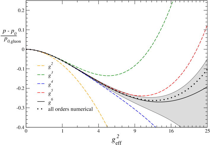
Figure 2: [color online] The behavior of the different orders of the weak coupling expansion of the large $N_{\rm f}$ pressure, Eq. (11), normalized to the pressure of free gluons $p_{0,\mathrm{gluon}}=d_{A}\pi^{2}T^{4}/45$ and plotted together with the all orders numerical result of Ref. Ipp et al. (2003). All the results are evaluated with the renormalization scale $\bar{\Lambda}=e^{-\gamma_{\rm E}}\pi T$, corresponding to the canonical ‘optimal’ scale of Ref. Kajantie et al. (1997). For the $g^{6}$ curve, we also display the effects of varying the renormalization scale by a factor $e^{\gamma_{\rm E}}\approx 1.78$, which corresponds to the shaded grey area. Note that when viewing the pressure as a function of the coupling, also the all orders numerical result has an explicit dependence on the renormalization scale, which only vanishes when taking the running of $g_{\mathrm{eff}}^{2}$ into account. This implies that the grey area is not to be compared to the all orders result, but is displayed only to give an idea of the size of the scale dependence of the perturbative result.

Finally, the $p_{0}\neq 0$ piece of $K_{4}$, $M_{4}^{\prime}$, is IR finite and in fact closely analogous to $M_{4}^{3,(p_{0}=0)}$. It is given by

$$M_{4}^{\prime} = 9\pi\sum_{n=1}^{\infty}\int\frac{d^{3}p}{(2\pi)^{3}}\int_{0}^{\infty}dr\,ds\,dt$$ (71)

$$\left[5+\frac{3}{p^{2}}\left(\partial_{r}^{2}+\partial_{s}^{2}+\partial_{t}^{2}\right)+\frac{5}{p^{4}}\left(\partial_{r}^{2}\partial_{s}^{2}+\partial_{r}^{2}\partial_{t}^{2}+\partial_{s}^{2}\partial_{t}^{2}\right)+\frac{3}{p^{6}}\partial_{r}^{2}\partial_{s}^{2}\partial_{t}^{2}\right]\left(\frac{\sin(pr)}{pr}\frac{\sin(ps)}{ps}\frac{\sin(pt)}{pt}\right)$$

$$\times\,\,\mathrm{e}^{-n(r+s+t)}\left(\mathrm{csch}\,r-\frac{1}{r}+\frac{r}{6}\right)\left(\mathrm{csch}\,s-\frac{1}{s}+\frac{s}{6}\right)\left(\mathrm{csch}\,t-\frac{1}{t}+\frac{t}{6}\right)$$

$$= 0.00003234178,$$

where the $r$, $s$ and $t$ derivatives again act only on the $\sin(px)/(px)$ terms.

Pulling all the pieces together, we find for the entire $K_{4}$ integral

$$K_{4} = \frac{T_{F}^{3}T^{4}}{135(2\pi)^{4}}\times 27.55287622.$$ (72)

IV Discussion and conclusions

In the previous Section, we have evaluated all of the integrals $K_{i}$ needed in constructing a result for the function $p_{6}$ of Eq. (11). Collecting everything with the help of Eqs. (21) and (30), we now finally obtain for the quantity

$$p_{6} = -\frac{800}{9}\ln^{2}\frac{\bar{\Lambda}}{4\pi T}-\frac{16}{3}\bigg{(}\frac{5}{3}+20\gamma_{\rm E}-88\ln 2$$

$$+ \frac{80}{3}\frac{\zeta^{\prime}(-1)}{\zeta(-1)}-\frac{40}{3}\frac{\zeta^{\prime}(-3)}{\zeta(-3)}\bigg{)}\ln\frac{\bar{\Lambda}}{4\pi T}+296.055373.$$

From here, we may also read off the leading large $N_{\rm f}$ behavior of the function $q_{c}(N_{\rm f})$ defined in Eq. (6.11) of Ref. Kajantie et al. (2003a),

$$q_{c}(N_{\rm f}) = 0.469861169\,N_{\rm f}^{3}+{\mathcal{O}}(N_{\rm f}^{2}),$$ (74)

as well as the coefficient $C_{6}$ defined in Ref. Ipp and Rebhan (2003),

$$C_{6} = 21.8597689.$$ (75)

It is quite reassuring that our result turned out to lie within the error bars of the very non-trivial numerical estimate $C_{6}=20(2)$ of Ref. Ipp and Rebhan (2003).

The above result can be contrasted on one hand with the exact numerical solution of the large $N_{\rm f}$ pressure Ipp et al. (2003), and on the other hand to the previous terms in the expansion of Eq. (11). In Fig. 2, we perform both comparisons, displaying the perturbative result for the pressure to various orders as a function of the effective coupling $g_{\mathrm{eff}}$, and comparing it at the same time to the all orders resummation of Ref. Ipp et al. (2003). As noted already in previous studies Ipp et al. (2003); Ipp and Rebhan (2003), the convergence of the weak coupling expansion seems quite impressive: The region of applicability of the result clearly increases order by order, and it is only for relatively large values of the effective coupling, $g_{\mathrm{eff}}^{2}\gtrsim 20$, that the renormalization scale dependence of the order $g^{6}$ result becomes strong enough to completely ruin its predictive power.

The good convergence properties of the large $N_{\rm f}$ pressure seem to indicate that in this case, the small parameter in the weak coupling expansion is really $g_{\mathrm{eff}}^{2}/(4\pi)^{2}$, as can indeed be verified from Eq. (11). This should be contrasted to the case of full QCD, where the EQCD contributions come with an associated expansion parameter $g$, while the MQCD ones are completely non-perturbative. Remarkably, in the large $N_{\rm f}$ limit, even the effective theory contributions organize themselves in the form of $g_{\mathrm{eff}}^{3}$ times a series expansion in $g_{\mathrm{eff}}^{2}/(4\pi)^{2}$. This can be seen to follow from the fact that in the large $N_{\rm f}$ limit, EQCD is a free theory . Its contribution to the pressure has the form $m_{\rm E}^{3}\times f(g_{3}^{2}/m_{\rm E})$, where $m_{\rm E}\sim g$ is the mass parameter and $g_{3}^{2}\sim g^{2}$ the gauge coupling constant of EQCD, both having weak coupling expansions in powers of $g^{2}/(4\pi)^{2}$. In the large $N_{\rm f}$ limit, the ratio $g_{3}^{2}/m_{\rm E}$ behaves as $1/N_{\rm f}$, implying that the pressure of EQCD is then indeed merely a number times $m_{\rm E}^{3}$, and therefore contributes to the pressure of the full theory as $g_{\mathrm{eff}}^{3}$ times an expansion in $g_{\mathrm{eff}}^{2}/(4\pi)^{2}$. Finally, the pressure of MQCD is entirely subleading in the large $N_{\rm f}$ limit.

Apart from providing the coefficient of the $N_{\rm f}^{3}g^{6}$ term in the expansion of the QCD pressure, our work has demonstrated the applicability of the computational methods developed for lower order calculations in Refs. Arnold and Zhai (1994, 1995) and for the case of scalar $\phi^{4}$ theory in Ref. Gynther et al. (2007) in tackling four-loop computations in QCD. We have been able to perform our work semi-analytically, dealing with all UV and IR divergent parts and logarithms of the renormalization scale analytically in dimensional regularization, and evaluating the remaining finite parts numerically to a high accuracy. At worst, we have had to deal with two-fold numerical integrals, which is a very modest challenge for state of the art computing facilities.

The success of the calculation performed in this paper encourages one to pursue further pieces of the $g^{6}$ coefficient of the QCD pressure using similar machinery. In particular, the term proportional to $N_{\rm f}^{2}g^{6}$ in the result consists of a reasonably limited set of diagrams, a large number of which seem amenable to an analogous treatment. Beyond this, the task rapidly becomes much more complicated, and an approach based on computer algebra methods proves necessary.

References

• Aoki et al. (2006) Y. Aoki, Z. Fodor, S. D. Katz, and K. K. Szabo, JHEP 01, 089 (2006), eprint hep-lat/0510084.
• Cheng et al. (2008) M. Cheng et al., Phys. Rev. D77, 014511 (2008), eprint 0710.0354.
• Kajantie et al. (2003a) K. Kajantie, M. Laine, K. Rummukainen, and Y. Schroder, Phys. Rev. D67, 105008 (2003a), eprint hep-ph/0211321.
• Vuorinen (2003) A. Vuorinen, Phys. Rev. D68, 054017 (2003), eprint hep-ph/0305183.
• Chesler et al. (2009) P. M. Chesler, A. Gynther, and A. Vuorinen (2009), eprint 0906.3052.
• Laine and Schroder (2005) M. Laine and Y. Schroder, JHEP 03, 067 (2005), eprint hep-ph/0503061.
• Carrington et al. (2008) M. E. Carrington, A. Gynther, and D. Pickering, Phys. Rev. D78, 045018 (2008), eprint 0805.0170.
• Braaten and Nieto (1996) E. Braaten and A. Nieto, Phys. Rev. D53, 3421 (1996), eprint hep-ph/9510408.
• Kajantie et al. (2003b) K. Kajantie, M. Laine, K. Rummukainen, and Y. Schroder, JHEP 04, 036 (2003b), eprint hep-ph/0304048.
• Di Renzo et al. (2006) F. Di Renzo, M. Laine, V. Miccio, Y. Schroder, and C. Torrero, JHEP 07, 026 (2006), eprint hep-ph/0605042.
• Hietanen et al. (2005) A. Hietanen, K. Kajantie, M. Laine, K. Rummukainen, and Y. Schroder, JHEP 01, 013 (2005), eprint hep-lat/0412008.
• Hietanen and Kurkela (2006) A. Hietanen and A. Kurkela, JHEP 11, 060 (2006), eprint hep-lat/0609015.
• Laine (2003) M. Laine (2003), eprint hep-ph/0301011.
• Gynther et al. (2007) A. Gynther, M. Laine, Y. Schroder, C. Torrero, and A. Vuorinen, JHEP 04, 094 (2007), eprint hep-ph/0703307.
• Andersen et al. (2009) J. O. Andersen, L. Kyllingstad, and L. E. Leganger (2009), eprint 0903.4596.
• Arnold and Zhai (1994) P. Arnold and C.-X. Zhai, Phys. Rev. D50, 7603 (1994), eprint hep-ph/9408276.
• Arnold and Zhai (1995) P. Arnold and C.-x. Zhai, Phys. Rev. D51, 1906 (1995), eprint hep-ph/9410360.
• Moore (2002) G. D. Moore, JHEP 10, 055 (2002), eprint hep-ph/0209190.
• Ipp et al. (2003) A. Ipp, G. D. Moore, and A. Rebhan, JHEP 01, 037 (2003), eprint hep-ph/0301057.
• Ipp and Rebhan (2003) A. Ipp and A. Rebhan, JHEP 06, 032 (2003), eprint hep-ph/0305030.
• Zhai and Kastening (1995) C.-x. Zhai and B. M. Kastening, Phys. Rev. D52, 7232 (1995), eprint hep-ph/9507380.
• Kapusta and Gale (2006) J. I. Kapusta and C. Gale, Finite-temperature field theory: Principles and applications (Cambridge, UK: Univ. Pr., 2006).
• Kajantie et al. (1997) K. Kajantie, M. Laine, K. Rummukainen, and M. E. Shaposhnikov, Nucl. Phys. B503, 357 (1997), eprint hep-ph/9704416.