Coreless vorticity in multicomponent Bose and Fermi superfluids

Abstract

We consider quantized vortices in two-component Bose-Einstein condensates and three-component Fermi gases with attractive interactions. In these systems, the vortex core can be either empty (normal in the fermion case) or filled with another superfluid. We determine critical values of the parameters – chemical potentials, scattering lengths and, for Fermi gases, temperature – at which a phase transition between the two types of vortices occurs. Population imbalance can lead to superfluid core (coreless) vorticity in multicomponent superfluids which otherwise support only usual vortices. For multicomponent Fermi gases, we construct the phase diagram including regions of coreless vorticity. We extend our results to trapped bosons and fermions using an appropriate local approximation, which goes beyond the usual Thomas-Fermi approximation for trapped bosons.

I Introduction

Properties of quantized vortex cores in superfluids have been actively researched for many years. For example, it was realized CDM that in type II superconductors there are low-energy states bound to the core and their effect on the local density of states was studied experimentally vscexp and theoretically vscth . More recently, observations of quantized vortices provided key evidence for superfluidity in both single component Bose-Einstein condensates (BECs) and two-component superfluid Fermi gases, where vortex cores are detected as regions of suppressed particle density varrbec ; varrfg . The core states in Fermi gases were considered in vortBECBCS .

The situation in unconventional superfluids is more complex. For instance, in superfluid ³He-B the vortex core is in a ferromagnetic superfluid state vHe3 . In high-temperature superconductors with $d$-wave order parameter an $s$-wave component must be present in the core dswave . In a color superconductor – high-density, low-temperature quark matter – there are many distinct fermion species (components) that can pair up, leading to two types of vortices – Abelian and non-Abelian colvor . Similarly, spinor atomic BECs having several bosonic components host, in addition to vortices, other types of topological excitations such as hedgehogs and skyrmions BECrev . This cannot happen, however, if the symmetry between the components is explicitly broken, in which case only vortices are possible.

Consider, for example, a three-component Fermi gas, which can support three distinct superfluid states ptm ; CY , with a vortex in superfluid $S_{1}$. The core of the vortex can be in the normal state, as for a two-component Fermi gas, or it can condense into one of the two other superfluid states – see Fig. 1. In view of current efforts to achieve superfluidity in three-component Fermi gases 3fge1 ; 3fge2 , it is important to understand which of these scenarios is realized and/or how to drive the transition between normal- and superfluid-core vortices. Similarly, competition between empty- and filled-core vortices takes place in a two-component BEC (2BEC). In fact, filled-core vortices have been experimentally observed vortexp ; vortexp2 , and their properties are in the focus of numerous theoretical studies stabcond1 ; stabcond2 ; tfavort ; binary ; tfaempty – see Ref. BECrev, for a review.

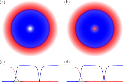
Figure 1: Order parameters for normal-core [panels (a) and (c)] and superfluid-core [(b) and (d)] vortices in multicomponent BECs and Fermi gases. Colors distinguish different superfluids. Top row: qualitative behavior of the order parameters in a plane of a trapped superfluid. Color intensity is proportional to the local value of the order parameters. Bottom row: profiles of the condensate wave functions in the absence of trapping.

In this paper, we study vortices in 2BECs and three-component Fermi gases. We show that both empty-(normal-) and filled-(superfluid-)core vortices can be realized depending on the parameters characterizing the bosonic (fermionic) system: chemical potentials, scattering lengths, and temperature in the case of fermions. We first focus on 2BEC at zero temperature and derive, using Gross-Pitaevskii equations, the critical relationship between the parameters of the system which determines whether the vortex is empty or filled. Fermions at sufficiently high temperature can be analyzed in a similar manner with the help of the Ginzburg-Landau expansion. This enables us to find a condition for the normal- to superfluid-core transition for vortices in a three-component Fermi gas. In particular, for balanced systems with equal populations of three fermion species, we explicitly obtain the critical temperature for this transition. We first consider bosons and fermions in the absence of an external potential, then extend our results to trapped systems. We further discuss the validity of the widely used Thomas-Fermi and local density approximations for analyzing vortex cores in trapped condensates.

II Two-component Bose system

The low temperature properties of a BEC are well described in terms of a condensate wave function $\Psi$ which obeys the Gross-Pitaevskii equation, which captures the effects of interactions at the mean field level. First, let us treat a 2BEC free of the trapping potential. The coupled Gross-Pitaevskii equations for the wave functions $\Psi_{i}$, $i=1,2$, of the two condensates in a stationary state can be obtained by minimizing the following energy density functional BECrev :

$$\begin{split}E=&\sum_{i=1}^{2}\left[\frac{1}{2m_{i}}|\nabla\Psi_{i}|^{2}-\mu_{i}|\Psi_{i}|^{2}+\frac{u_{ii}}{2}|\Psi_{i}|^{4}\right]\\ &+u_{12}|\Psi_{1}|^{2}|\Psi_{2}|^{2},\end{split}$$ (1)

where $m_{i}$ and $\mu_{i}$ are the atomic masses and chemical potentials, respectively. The coupling constants $u_{ij}$ are related to the (positive) scattering lengths $a_{ij}$

$$u_{ij}=2\pi a_{ij}\left(1/m_{i}+1/m_{j}\right).$$ (2)

We consider the case in which the two BECs phase separate (i.e., $u_{12}^{2}-u_{11}u_{22}>0$) and assume that there is a vortex line along the $z$ axis in condensate 1. Then the wave function of the condensate has the form

$$\Psi_{1}(\mathbf{r},\phi)=\sqrt{\frac{\mu_{1}}{u_{11}}}e^{i\phi}f\left(\frac{r}{\xi_{1}}\right),$$ (3)

where $\xi_{1}=1/\sqrt{2m_{1}\mu_{1}}$ is the healing length and $\mathbf{r}=(r,z)$. The profile function $f(x)$ is the solution of the non-linear differential equation (primes denote derivatives)

$$f^{\prime\prime}+\frac{f^{\prime}}{x}-\frac{f}{x^{2}}=-f+f^{3}$$ (4)

with the boundary conditions $f(0)=0$ and $f(x)\to 1$ as $x\to\infty$.

Condensate 2 fills the core of the vortex in condensate 1 when this is energetically favorable. At the transition from and empty ($\Psi_{2}=0$ in the core) to a filled core ($\Psi_{2}\neq 0$), $\Psi_{2}$ is infinitesimally small. The energy difference between filled and empty core states to the lowest order in $\Psi_{2}$ is

$$\delta E=L_{z}\!\int\!d^{2}r\left[\frac{1}{2m_{2}}|\nabla\Psi_{2}|^{2}+u_{12}|\Psi_{1}|^{2}|\Psi_{2}|^{2}-\mu_{2}|\Psi_{2}|^{2}\right],$$ (5)

where $L_{z}$ is the size of the system in the $z$ direction. We can neglect the effect of $\Psi_{2}$ on $\Psi_{1}$, since it is of higher order in $\Psi_{2}$. This equation can be rewritten as

$$\delta E=L_{z}\xi_{1}^{2}\left[\frac{u_{12}}{u_{11}}\epsilon_{0}(\beta_{r})\mu_{1}-\mu_{2}\right]\int\!d^{2}\rho\,|\Psi_{2}|^{2}\,,$$ (6)

where $\epsilon_{0}$ is the (dimensionless) ground state energy of the following two-dimensional Schrödinger equation:

$$-\beta_{r}\nabla^{2}\Psi_{2}(\rho,\phi)+f^{2}(\rho)\Psi_{2}(\rho,\phi)=\epsilon_{0}\Psi_{2}(\rho,\phi)$$ (7)

with $\rho=r/\xi_{1}$ and the “inverse mass” being $\beta_{r}=m_{1}u_{11}/m_{2}u_{12}$. The analysis reported in Appendix A shows that a good approximation for the monotonically increasing function $\epsilon_{0}(\beta_{r})$ is given by (see also Fig. 2)

$$\epsilon_{0}(\beta_{r})\simeq\left\{\begin{array}[]{lcl}2\sqrt{\beta_{r}}c_{0}-\frac{1}{2}\beta_{r}+\frac{16c_{0}^{2}-4}{32c_{0}}\beta_{r}^{3/2},&&\beta_{r}\lesssim 3,\\ 1-4e^{-2\gamma_{E}}c_{0}^{2}\beta_{r}e^{-2\sqrt{\beta_{r}}\arctan\left[c_{0}^{2}2\sqrt{\beta_{r}}\right]},&&\beta_{r}\gtrsim 3,\end{array}\right.$$ (8)

where $\gamma_{E}$ is Euler’s constant and $c_{0}=f^{\prime}(0)\simeq 0.58319$.

Figure 2: Ground state energy $\epsilon_{0}$ of Schrödinger Eq. (7) as a function of the inverse mass $\beta_{r}$. Solid line: numerical calculation. Dotted (dashed) line: analytical approximation Eq. (8) for $\beta_{r}\lesssim 3$ ($\beta_{r}\gtrsim 3$). Inset: relative deviations between the approximations and the numerical results.

As an example, consider a system with $m_{1}=m_{2}$ and $\mu_{1}=\mu_{2}$. Then Eqs. (6) and (8) show that for $a_{22}<a_{12}<a_{11}$ a coreless vortex in superfluid 1 is more stable than a coreless vortex in superfluid 2, since the latter state has higher energy. This is in agreement with the experimental findings of Ref. vortexp, .

More generally, the sign of the term in square brackets in Eq. (6) determines the stable core state. If it is positive, it costs energy to fill the core. Hence the core is empty if

$$\frac{u_{11}}{u_{12}}<\frac{\mu_{1}}{\mu_{2}}\epsilon_{0}\left(\frac{m_{1}u_{11}}{m_{2}u_{12}}\right).$$ (9)

In other words, Eq. (9) defines a surface in the space of parameters that separates the regions of empty and filled core vorticities. For example, we see that population imbalance, which modifies the ratio $\mu_{1}/\mu_{2}$, impedes coreless vorticity in one of the condensates while favoring it in the other, as seen by exchanging $1\leftrightarrow 2$. Analogous conclusions hold for the ratio between intra- and interspecies scattering length and the ratio of masses. Interestingly, while our calculations are performed in the thermodynamic limit, qualitatively similar conclusions were reached in Refs. stabcond1, -stabcond2, , where stability conditions were derived for vortices in a small trapped condensate.

Now, let us analyze the effects due to an external potential. For simplicity, we consider a spherically symmetric harmonic trap $V(\mathbf{r})$ and assume, without loss of generality, that condensate 1 occupies its center, while superfluid 2 forms a shell around it. Vortices in trapped 2BEC have been previously studied in Refs. tfavort, ; binary, ; tfaempty, using the Thomas-Fermi approximation (TFA). In this approximation only the angular part of the kinetic energy terms in Eqs. (1) and (5) is kept. Then, the wave functions $\Psi_{i}$, $i=1,2$ of the condensates are obtained from those in the absence of the trapping potential via the replacement $\mu_{i}\to\mu_{i}(\mathbf{r})\equiv\mu_{i}(0)-V(\mathbf{r})$, i.e., the trapped 2BEC is taken to be locally uniform. This is justified in large condensates, $R_{i}\gg\xi_{i}$, where $R_{i}$ and $\xi_{i}$ are condensate sizes and healing lengths, respectively.

Neglecting the radial parts of the kinetic energy, however, is a good approximation only when $\Psi_{i}$ varies over distances much larger than $\xi_{i}$. As we have seen above, this is not the case close to the vortex line, where both $\Psi_{1}$ and $\Psi_{2}$ vary on the scale $\xi_{1}$, see Eqs. (4) and (7). We therefore expect the TFA to break down in determining the state in the vortex core. Indeed, one of its artifacts is that $\Psi_{1}$ is identically zero in a finite region inside the core tfavort ; tfaempty . This implies that the second term in Eq. (5) vanishes too, while the last term always makes it energetically favorable for the otherwise empty core to be filled by the second superfluid. Thus, the question whether the core is empty or filled cannot be resolved within the TFA, prompting arbitrary assumptions of filled tfavort ; binary and empty tfaempty core vortices in the literature.

This question, as we now show, can be accurately answered for large condensates by combining our approach with the local uniformity assumption discussed above. For example, let us work out the condition under which an empty core vortex is realized in superfluid 1 for $m_{1}=m_{2}$. The separation of scales, $R_{i}\gg\xi_{i}$, allows us to describe the vortex profile by Eq. (3) with $\mu_{i}\to\mu_{i}(\mathbf{r})$. In other words, we neglect gradients of $\mu_{1}(\mathbf{r})$ but not of $f(r)$. This approximation is valid at distances $L\gg\xi_{1}$ from the interfaces between the condensates becint . In a plane perpendicular to the vortex line, the wave functions$\Psi_{i}$ looks like Figs. 1(c) and (d), except for the curvature imposed by the trapping potential. $\Psi_{1}(\mathbf{r},\phi)$ changes rapidly near the core as $r$ varies over distances $r\sim\xi_{1}$ and is smooth on this scale when moving along the $z$ axis (vortex line).

Therefore, the stability of an empty core vortex for any $z$ is determined by Eq. (9) with $\mu_{i}\to\mu_{i}(r_{c},z)$, $r_{c}$ being the position of the core. We obtain

$$\frac{\mu_{2}(r_{c},z)}{\mu_{1}(r_{c},z)}<\frac{a_{12}}{a_{11}}\,\epsilon_{0}\!\left(\frac{a_{11}}{a_{12}}\right),$$ (10)

where we took into account $m_{1}=m_{2}=m$ and $u_{ij}=4\pi a_{ij}/m$ – see Eq. (2). Further, one can show that $\mu_{2}(0)>\mu_{1}(0)$ is necessary for superfluid 1 to occupy the center of the trap tfaempty ; note1 . It follows that the left-hand side of Eq. (10) is a monotonically increasing function of $|z|$, i.e., it reaches its maximum at the interface between the two condensates. The position $\mathbf{r}_{in}$ of the interface is determined from the condition $\mu_{2}(\mathbf{r}_{in})/\mu_{1}(\mathbf{r}_{in})=\sqrt{a_{22}/a_{11}}$ obtained by equating the pressures on the two sides tfaempty ; note1 , so that Eq. (10) becomes

$$\sqrt{\frac{a_{22}}{a_{11}}}<\frac{a_{12}}{a_{11}}\,\epsilon_{0}\!\left(\frac{a_{11}}{a_{12}}\right).$$ (11)

If this inequality holds, it costs energy to introduce the second condensate everywhere along the vortex core and the empty vortex is the stable state. Otherwise, the core is partially or fully filled. Since the left-hand side of Eq. (10) is larger at the interface, when varying the scattering lengths the core will be filled starting from the interface between the condensates towards the trap center. Using Eq. (8) and the experimental values reported in Ref. vortexp, , we find that condition (11) is violated in this experiment. This invalidates the approach of Ref. tfaempty, for the description of this experiment based on an empty core assumption.

A few comments are in order about the present derivation. We have not used anywhere the condition $a_{12}^{2}-a_{11}a_{22}>0$ that ensures phase separation in the absence of external potentials. For trapped 2BEC, phase separation can occur as long as $a_{12}>0$, although if $a_{12}^{2}-a_{11}a_{22}<0$ a coexistence region is present binary . In this case our analysis applies at distances $L\gg\xi_{i}$ from the coexistence region, but the inequality (11) is always violated since $\epsilon_{0}<1$ – see Eq. (8). This means that empty vortices are possible only in phase-separated condensates. More generally, as discussed above, to obtain Eq. (11) we use locally the result derived in the thermodynamic limit. This approximation is valid assuming slow variation of the wave functions along the vortex line. This assumption breaks down near the interface between the two phases, and even in fully phase-separated 2BEC the regions where the vortex core meets the interface are beyond the reach of the present approach.

III Three-component Fermi system

The treatment presented above can be applied to the study of a vortex in a multicomponent Fermi system at sufficiently high temperature. Consider, in particular, a three-component system at weak coupling near second order phase transition lines. The Ginzburg-Landau (GL) expansion for the thermodynamic potential $\Omega$ is CY

$$\frac{\Omega-\Omega_{N}}{\nu} = \sum_{i=1}^{2}\left\{\alpha_{i}|\Delta_{i}|^{2}+\frac{\beta_{ii}}{2}\left[|\Delta_{i}|^{4}+\frac{v_{F}^{2}}{3}|\nabla\Delta_{i}|^{2}\right]\right\}$$ (12)

$$+\beta_{12}|\Delta_{1}|^{2}|\Delta_{2}|^{2},$$

where $\Omega_{N}$ is the normal-state potential, $\nu$ is the density of states at the Fermi energy, $v_{F}$ is the Fermi velocity, and $\Delta_{i}$ is the order parameter describing pairing of particles belonging to species $j$ and $k$ with $j$, $k$, and $i$ all different.

The coefficients $\alpha_{i}$, $\beta_{ij}$ in Eq. (12) are

$$h_{1} = \mu_{3}-\mu_{2}\,,\quad h_{2}=\mu_{3}-\mu_{1}\,,$$

$$\alpha_{i} = \ln\frac{T}{T_{c_{i}}}+\mathrm{Re}\,\psi\left(\frac{1}{2}+\frac{\mathrm{i}h_{i}}{4\pi T}\right)-\psi\left(\frac{1}{2}\right),$$ (13)

$$\beta_{ij} = \frac{1}{h_{i}-h_{j}}\frac{1}{4\pi T}\mathrm{Im}\bigg{[}\psi^{\prime}\left(\frac{1}{2}+\frac{\mathrm{i}h_{j}}{4\pi T}\right)\bigg{]}+(j\to i),$$

where $\mu_{i}$ are the chemical potentials of the three species, $\psi$ is the digamma function, $\beta_{ii}$ is obtained from $\beta_{ij}$ in the limit $h_{j}\to h_{i}$, and $T_{c_{1}}$ ($T_{c_{2}}$) is the critical temperature for the normal-superfluid transition for a two-component gas of species 2 and 3 (1 and 3). With no loss of generality we assume $T_{c_{1}}>T_{c_{2}}$. For simplicity, we neglect the weakest of the three possible interactions, say between species 1 and 2 (recall that due to Pauli exclusion principle only interspecies scattering is possible in the $s$-wave channel). Then, there are only three main phases of the three-component system – the normal phase N ($\Delta_{1}=\Delta_{2}=0$), superfluid $S_{1}$ ($\Delta_{1}\neq 0,\Delta_{2}=0$), and superfluid $S_{2}$ ($\Delta_{1}=0,\Delta_{2}\neq 0$). The applicability of the GL expansion requires $T\gtrsim 0.56T_{c_{1}}$ and $|h_{i}|/4\pi T\lesssim 0.30$. In this regime $\beta_{ij}>0$, indicating repulsion (this is a consequence of Pauli exclusion), and $\beta_{12}^{2}-\beta_{1}\beta_{2}\geq 0$, leading to phase separation between the superfluid states. The first-order $S_{1}$-$S_{2}$ transition is accessible within the GL description when $T_{c_{1}}-T_{c_{2}}\ll T_{c_{2}}$ and $T_{c_{2}}-T\ll T_{c_{2}}$ – see Ref. CY, for more details.

Comparison of Eqs. (1) and (12) shows that, up to a redefinition of the various parameters, the energy argument discussed in Sec. II can be applied to the thermodynamics of the three-component Fermi gas. For example, a vortex in superfluid $S_{1}$ is described by the order parameter [cf. Eq. (3)]

$$\Delta_{1}(\mathbf{r},\phi)=\sqrt{\frac{-\alpha_{1}}{\beta_{11}}}e^{i\phi}f\left(\frac{r}{\xi_{1}}\right)$$ (14)

with the coherence length $\xi_{1}=v_{F}\sqrt{\beta_{11}/6(-\alpha_{1})}$.

Repeating the previous analysis for such a vortex we find the following condition for the second-order phase transition between normal and superfluid core (or equivalently between standard and coreless vortex):

$$\alpha_{2}-\alpha_{1}\frac{\beta_{12}}{\beta_{11}}\,\epsilon_{0}\!\left(\frac{\beta_{22}}{\beta_{12}}\right)=0,$$ (15)

where the function $\epsilon_{0}(x)$ is given by Eq. (8). The first term in Eq. (15) originates from the energy gained by condensation of the originally uncondensed species. The condensation takes place in the core region, where pairs of the first superfluid are broken due to vorticity. The second term is due to the energy costs associated with deforming the order parameter $\Delta_{2}$ [kinetic energy in Eq. (7)] and the repulsive interaction between the two superfluids (potential energy).

At a given temperature $T<T_{c_{2}}$, Eq. (15) determines the area in the $h_{1}$-$h_{2}$ space where the core is filled. It can be satisfied only in the central region of this space where both coefficients $\alpha_{1,2}$ are negative, i.e., when condensation is in principle possible in both channels. We show two examples of phase diagrams in Figs. 3 and 4. At a temperature close to $T_{c_{2}}$ (Fig. 3) the core is filled only in small regions around the first order phase transition between the two superfluid states. As the temperature is lowered (Fig. 4) the regions where superfluidity is possible expand, and so do the regions of coreless vorticity. In particular, as the temperature decreases, coreless vortices become possible even in balanced systems with equal populations ($h_{1}=h_{2}=0$). In this case the coefficients $\beta_{ij}$ all coincide and from Eq. (15) we find that the temperature $T_{o}$ for the onset of coreless vorticity is related to the superfluid critical temperatures as

$$T_{o}=T_{c_{2}}\left(\frac{T_{c_{2}}}{T_{c_{1}}}\right)^{\gamma},\quad\gamma=\frac{\epsilon_{0}(1)}{1-\epsilon_{0}(1)}\simeq 2.92\,.$$ (16)

Above $T_{o}$ the core is in a normal state, while for $T<T_{o}$ it is superfluid.

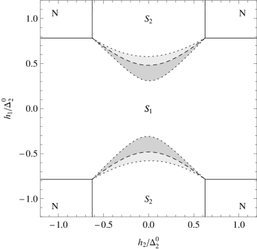
Figure 3: High temperature ($T=0.93T_{c2}$) phase diagram for a three-component Fermi gas with $T_{c_{1}}/T_{c_{2}}=1.04$ in the plane of chemical potential differences $h_{i}$. Solid lines: second-order normal-superfluid phase transitions. Dashed lines: first-order transition between the two superfluid states. In dark grey are the regions where the core of a vortex in the $S_{1}$ superfluid is filled by the $S_{2}$ superfluid. Light grey: $S_{1}$ superfluid fills the $S_{2}$ vortex core.

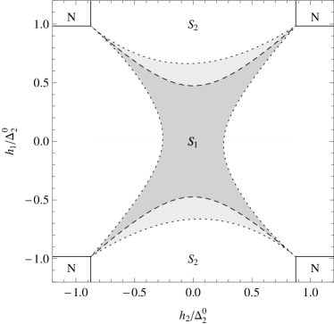
Figure 4: Phase diagram as in Fig. 3 but for a lower temperature ($T=0.85T_{c2}$). Note that now the coreless vortex state is present even for balanced gases with $h_{i}=0$.

Eq. (15) can be used to study trapped Fermi gases within the local density approximation (LDA) so long as condensate size $R$ is large compared to the coherence length $\xi_{1}$. Then, we can simply substitute local values of the critical temperatures $T_{c_{i}}(r)$ into Eq. (15) (note that chemical potential differences $h_{i}$ are position independent within LDA). The condition $R\gg\xi_{1}$ is satisfied if the total particle number $N_{t}$ is large enough. For a somewhat weak interaction $k_{F}|a_{s}|\simeq 0.5$ the condition on the particle number is $N_{t}\gg 10^{3}$, see Ref. CY, . We remind, however, that for imbalanced systems the presence of domain walls could require larger particle numbers for the LDA to be valid.

The above calculations are valid in the weak coupling regime near second order phase transitions. The latter requirement is satisfied for all relevant chemical potential differences if $T_{c_{1}}-T_{c_{2}}\ll T_{c_{2}}$ and $T$ is close to $T_{c_{2}}$. Relaxing these conditions will not alter the qualitative picture, although it will affect the quantitative results. For example, if the difference between the critical temperatures, $T_{c_{1}}-T_{c_{2}}$, is large, we expect the actual onset temperature $T_{o}$ to be smaller than that predicted by Eq. (16): at low temperature $T\to 0$ the order parameter in the core region rises on a length scale of the order of the Fermi wave length vortBECBCS ; ltv rather than the much longer (at weak coupling) coherence length. At lowest order this is equivalent to an increase of $c_{0}$ in, e.g., Eq. (8), which would lead to a higher value for $\epsilon_{0}(1)$ in Eq. (16) and hence a lower onset temperature.

IV Summary

We considered the empty- and filled-core vortex states in two-component BECs described by the Gross-Pitaevskii equations, as well as the normal- and superfluid-core vortices in three-component Fermi gases using a Ginzburg-Landau approach. In the absence of external potentials, we derived the conditions [Eq. (9) and (15) for Bose and Fermi systems, respectively] that determine the transition between the two states in terms of chemical potentials, scattering lengths and, for Fermi gases, temperature. In particular, we obtained a simple expression, Eq. (16), for the onset temperature of coreless vorticity in the population-balanced Fermi gas. We also established when the vortex core remains empty in trapped Bose systems, see Eq. (11), using a local approximation which goes beyond the usual Thomas-Fermi Approximation. We showed that, for equal masses of the components, empty vortices are possible only in phase-separated 2BECs and that in partially filled vortices the superfluid part of the core is in the region closer to the interface between the two condensates. We similarly applied our findings to trapped multicomponent Fermi gases within the Local Density Approximation and discussed the limits of validity of this approach. The detailed study of the superfluid core is left to future work, as is the extension of our results to Fermi-Bose mixtures.

Appendix A Calculation of the ground-state energy

In this Appendix we present the calculation of the ground-state energy $\epsilon_{0}$ of Eq. (7). The potential term $f^{2}(\rho)$ is not known explicitly, except for its behavior at small and large $x$. Indeed, near the origin a power series for $f(\rho)$ can be found in term of one unknown parameter, $c_{0}$, which is calculated using the boundary condition at infinity. The first few terms in this expansion are:

$$f(\rho)=c_{0}\rho-\frac{c_{0}}{8}\rho^{3}+\frac{c_{0}(1+8c_{0}^{2})}{192}\rho^{5}+O(\rho^{7})\,.$$ (17)

The coefficient $c_{0}\simeq 0.58319$ can be evaluated with great precision either numerically or with analytical methods c0ref . As $\rho\to+\infty$ the asymptotic expansion is:

$$f(\rho)=1-\frac{1}{2\rho^{2}}-\frac{9}{8\rho^{4}}+O(\rho^{-6})\,.$$ (18)

By appropriate rescalings, we show that this is sufficient to obtain analytical estimates for $\epsilon_{0}$ at small and large $\beta_{r}$ which, moreover, provide accurate estimates even at intermediate values.

A.1 Small $\beta_{r}$

The limit $\beta_{r}\to 0$ corresponds to a particle with large mass; therefore, its ground state wave functions does not extend far from the origin. This enables us to calculate $\epsilon_{0}$ perturbatively, using the harmonic oscillator as starting point. Indeed, after the rescaling $\rho=\beta_{r}^{1/4}c_{0}^{-1/2}x$, Eq. (7) becomes

$$-\nabla^{2}\Psi_{2}+\left[x^{2}+V_{\beta_{r}}(x)\right]\Psi_{2}=\tilde{\epsilon}_{0}\Psi_{2}$$ (19)

with $\tilde{\epsilon}_{0}=\epsilon_{0}/\sqrt{\beta_{r}}c_{0}$ and $V_{\beta_{r}}(x)$ the perturbation potential. The latter is defined as the potential term of Eq. (7), $f^{2}(\rho)$, minus the harmonic part. From Eq. (17) we find the first few terms in the small-$x$ expansion:

$$V_{\beta_{r}}(x)=-\sqrt{\beta_{r}}\frac{1}{4c_{0}}x^{4}+\beta_{r}\frac{5+16c_{0}^{2}}{192c_{0}^{2}}x^{6}+O(\beta_{r}^{3/2}x^{8})\,.$$ (20)

Consistently with the truncation of the potential $V_{\beta_{r}}$, we calculate $\tilde{\epsilon}_{0}$ to second order in the small parameter $\sqrt{\beta_{r}}$ via standard time-independent perturbation theory LLqm . Since the potential does not break 2D rotational symmetry, to calculate the correction to the ground state energy we only need to know the $s$-wave eigenvalues $\varepsilon_{n}$ and eigenfunctions $\psi_{n}$ of the 2D harmonic oscillator:

$$\begin{split}&\varepsilon_{n}=2(2n+1)\,,\\ &\psi_{n}(x)=\sqrt{2}e^{-x^{2}/2}L_{n}(x^{2})\,,\end{split}$$ (21)

where $L_{n}$ are the Laguerre polynomials. In calculating the matrix elements of the perturbation we use the identity

$$u^{n}=n!\sum_{i=0}^{n}(-1)^{i}\frac{n!}{(n-i)!i!}L_{i}(u)\,$$ (22)

which follows by induction from the recurrence relation for the Laguerre polynomials absteg . After straightforward algebra we find

$$\epsilon_{0}=2\sqrt{\beta_{r}}c_{0}-\frac{1}{2}\beta_{r}+\frac{16c_{0}^{2}-4}{32c_{0}}\beta_{r}^{3/2}+O(\beta_{r}^{2})\,.$$ (23)

Requiring the second term to be a small correction gives the condition $\beta_{r}\ll 5.44$; hence the expansion should be reliable up to $\beta_{r}$ of order 1. Indeed, both the calculation of the coefficient of the $\beta_{r}^{2}$ term ($\simeq 0.003)$ and comparison with numerics (see the end of this Appendix) show that Eq. (23) is still a good approximation even for $\beta_{r}\gtrsim 1$.

A.2 Large $\beta_{r}$

In the limit of large $\beta_{r}$ the kinetic term in Eq. (7) becomes dominant, which physically correspond to an almost free particle, and the (properly defined) potential $U(\rho)$ can be treated as a shallow one. Since $f^{2}(\rho)\to 1$ at large $\rho$, we define $U(\rho)=f^{2}(\rho)-1$ and $\varepsilon=1-\epsilon_{0}$, so that positive energies correspond to bound states. In two dimensions the ground state energy in a shallow potential depends exponentially on the inverse mass LLqm : $\varepsilon\propto\beta_{r}e^{-c\beta_{r}}$, where the constant $c\propto|\int d^{2}\rho\,U(\rho)|^{-1}$. This result holds when the integral converges, while in our case the integral is logarithmically divergent, see Eq. (18). We can adapt to the present situation the derivation of the above estimate for $\varepsilon$ presented in Ref. LLqm, , §45. We show at the end of this appendix that the expression thus obtained agrees well with numerical calculations.

We define

$$y=\sqrt{\frac{\varepsilon}{\beta_{r}}}\rho$$ (24)

and rewrite Eq. (7) as

$$\frac{1}{y}\left[y\Psi_{2}^{\prime}(y)\right]^{\prime}=U\left(y\right)\Psi_{2}(y)$$ (25)

with

$$U(y)=1+\frac{1}{\varepsilon}\left[f^{2}\left(\sqrt{\frac{\beta_{r}}{\varepsilon}}y\right)-1\right].$$ (26)

Here we include the eigenvalue term ($\propto\varepsilon$ in the original equation) into the potential energy $U$. In a small circle around the origin of radius $y_{0}$ the potential can be approximated as

$$U(y)\simeq-\frac{1}{\varepsilon}\,.$$ (27)

In this region the wave function can be taken as approximately constant, $\Psi_{2}=1$, and integrating both side of Eq. (25) gives

$$y_{0}\Psi_{2}^{\prime}(y_{0})=-\frac{1}{2\varepsilon}y_{0}^{2}\,.$$ (28)

To estimate $y_{0}$, we note that according to Eq. (17) the length scale over which the potential varies appreciably near the origin is $x\sim 1/c_{0}$, so we take $y_{0}=\sqrt{\varepsilon/\beta_{r}}/c_{0}$.

For $y\gg\sqrt{\varepsilon/\beta_{r}}$, the potential $U$ is approximately

$$U(y)\simeq 1-\frac{1}{\beta_{r}y^{2}}$$ (29)

and Eq. (25) has as solution the modified Bessel function of imaginary order $K_{i/\sqrt{\beta_{r}}}(y)$. We want to match its logarithmic derivative to the estimate in Eq. (28); to do so, we use the following approximate expression valid for $y,1/\sqrt{\beta_{r}}\ll 1$ bessim

$$K_{i/\sqrt{\beta_{r}}}(y)\simeq-\sqrt{\beta_{r}}\sin\left[\frac{1}{\sqrt{\beta_{r}}}\left(\log\frac{y}{2}+\gamma_{E}\right)\right].$$ (30)

Direct inspection of the matching condition at $y_{0}$ suggests taking $\varepsilon$ in the form

$$\varepsilon=4e^{-2\gamma_{E}}c_{0}^{2}\beta_{r}e^{-b\sqrt{\beta_{r}}}$$ (31)

for some parameter $b$. Then the matching condition reduces to

$$\frac{1}{\sqrt{\beta_{r}}\tan\left[b/2\right]}=\frac{1}{2c_{0}^{2}\beta_{r}}$$ (32)

and solving for $b$ we find

$$b=2\arctan\left[2c_{0}^{2}\sqrt{\beta_{r}}\right]\,.$$ (33)

Substituting this back into Eq. (31) we finally arrive at

$$\epsilon_{0}=1-4e^{-2\gamma_{E}}c_{0}^{2}\beta_{r}e^{-2\sqrt{\beta_{r}}\arctan\left[c_{0}^{2}2\sqrt{\beta_{r}}\right]}\,.$$ (34)

Note that, in agreement with Eq. (30), $K_{i/\sqrt{\beta_{r}}}(y)$ has an infinite number of zeros at (approximate) positions $y_{n}=2e^{-\pi n\sqrt{\beta_{r}}-\gamma_{E}}$, $n=1,2,3,\ldots$, and no other zeros at $y>y_{1}$. It is easy to check that $y_{n}<y_{0}$, so that the approximate wave function constructed in the course of this derivation has no zeros, as expected for the ground state.

To check the accuracy of the estimates in Eqs. (23) and (34), we also solve Eq. (7) numerically. That is, we first find a numerical solution to Eq. (4) for $f(x)$; then we find numerical estimates of the ground state energy of Eq. (7) for various $\beta_{r}$. Interpolation of these numerical results gives the solid curve in Fig. 2, where we also plot Eqs. (23) and (34) for comparison. Using Eq. (23) for $\beta_{r}\lesssim 3$ and Eq. (34) for $\beta_{r}\gtrsim 3$ gives estimates that deviate less than 1% from the numerics – see the inset of Fig. 2.

References

- (1) C. Caroli, P. G. de Gennes, J. Matricon, Phys. Lett. 9, 307 (1964).
- (2) H. F. Hess et al., Phys. Rev. Lett. 62, 214 (1989).
- (3) F. Gygi and M. Schlüter, Phys. Rev. Lett. 65, 1820 (1990); Phys. Rev. B 43, 7609 (1991).
- (4) M. R. Andrews et al., Science 273, 84 (1996).
- (5) M. W. Zwierlein et al., Nature 453, 1047 (2005).
- (6) M. Machida and T. Koyama, Phys. Rev. Lett. 94, 140401 (2005); R. Sensarma, M. Randeria, and T.-L. Ho, Phys. Rev. Lett. 96, 090403 (2006).
- (7) M. M. Salomaa and G. E. Volovik, Rev. Mod. Phys. 59, 533 (1987).
- (8) Y. Ren, J. Xu, and C. S. Ting, Phys. Rev. Lett. 74, 3680 (1995).
- (9) A.P. Balachandran, S. Digal, and T. Matsuura, Phys. Rev. D 73, 074009 (2006).
- (10) K. Kasamatsu, M. Tsubota, and M. Ueda, Int. J. Mod. Phys. B. 19, 1835 (2005).
- (11) T. Paananen, P. Torma, and J.-P. Martikainen, Phys. Rev. A 75, 023622 (2007).
- (12) G. Catelani and E. A. Yuzbashyan, Phys. Rev. A 78, 033615 (2008).
- (13) T. B. Ottenstein et al., Phys. Rev. Lett. 101, 203202 (2008).
- (14) J. H. Huckans et al., Phys. Rev. Lett. 102, 165302 (2009).
- (15) M. R. Matthews et al., Phys. Rev. Lett. 83, 2498 (1999).
- (16) B. P. Anderson et al., Phys. Rev. Lett. 85, 2857 (2000).
- (17) D. V. Skryabin, Phys. Rev. A 63, 013602 (2000).
- (18) J. J. Garcia-Ripoll and V. M. Perez-Garcia, Phys. Rev. Lett. 84, 4264 (2000); V. M. Perez-Garcia and J. J. Garcia-Ripoll, Phys. Rev. A 62, 033601 (2000).
- (19) D. M. Jezek, P. Capuzzi, and H. M. Cataldo, Phys. Rev. A 64, 023605 (2001).
- (20) T.-L. Ho and V. B. Shenoy, Phys. Rev. Lett. 77, 3276 (1996).
- (21) S. T. Chui, V. N. Ryzhov, and E. E. Tareyeva, Phys. Rev. A 63, 023605 (2001); JETP 91, 1183 (2000).
- (22) R. A. Barankov, Phys. Rev. A 66, 013612 (2002); B. Van Schaeybroeck, ibid. 78, 023624 (2008).
- (23) Note that the presence of a vortex does not significantly alter the chemical potentials and the intereface as it occupies a small fraction of the condensate. Therefore, one can use the TFA to determine these quantities.
- (24) L. Kramer and W. Pesch, Z. Physik 269, 59 (1974).
- (25) N. G. Berloff, J. Phys. A: Math. Gen. 37, 1617 (2004); B. Boisseau et al., J. Phys. A: Math. Theor. 40, F215 (2007).
- (26) L. D. Landau and E. M. Lifshitz, Quantum mechanics (Butterworth-Heinemann, Oxford, 1981).
- (27) See, e.g., M. Abramowitz and I. A. Stegun (eds.), Handbook of Mathematical Functions (Dover, New York, 1964).
- (28) T. M. Dunster, SIAM J. Math. Anal. 21, 995 (1990).