AEI-2009-092

Quasilocal formalism and thermodynamics of asymptotically flat black objects

Dumitru Astefanesei^a, Robert B. Mann^b,c Maria J. Rodriguez^a Cristian Stelea^d

^a Max-Planck-Institut für Gravitationsphysik, Albert-Einstein-Institut, 14476 Golm, Germany
^bPerimeter Institute for Theoretical Physics, Ontario N2J 2W9, Canada
^c Department of Physics, University of Waterloo Waterloo, Ontario N2L 3G1, Canada
^d Department of Physics and Astronomy, University of British Columbia, Vancouver, Canada

dumitru@aei.mpg.de, mann@avatar.uwaterloo.ca,
maria.rodriguez@aei.mpg.de, stelea@phas.ubc.ca

We study the properties of 5-dimensional black objects by using the renormalized boundary stress-tensor for locally asymptotically flat spacetimes. This provides a more refined form of the quasilocal formalism which is useful for a holographic interpretation of asymptotically flat gravity. We apply this technique to examine the thermodynamic properties of black holes, black rings, and black strings. The advantage of using this method is that we can go beyond the ‘thin ring’ approximation and compute the boundary stress tensor for any general (thin or fat) black ring solution. We argue that the boundary stress tensor encodes the necessarily information to distinguish between black objects with different horizon topologies in the bulk. We also study in detail the susy black ring and clarify the relation between the asymptotic charges and the charges defined at the horizon. Furthermore, we obtain the balance condition for ‘thin’ dipole black rings.

1 Introduction

A remarkable development in theoretical physics was the discovery of a close relationship between the laws of thermodynamics and certain laws of black hole physics. The black hole represents the equilibrium end state of gravitational collapse, so on general grounds we might expect it to be the state of maximum entropy for a self-gravitating system. The relationship between thermodynamic entropy and the area of an event horizon is one of the most robust and surprising results in gravitational physics.

In a very basic sense, gravitational entropy can be regarded as arising from the Gibbs-Duhem relation applied to the path-integral formulation of quantum gravity [1]. In the semiclassical limit this yields a relationship between gravitational entropy and other relevant thermodynamic quantities, such as mass, angular momentum, and other conserved charges.

This relationship was first explored in the context of black holes by Gibbons and Hawking [2], who argued that the thermodynamical potential is equal to the Euclidean gravitational action multiplied by the temperature. In this approach, the partition function for the gravitational field is defined by a sum over all smooth Euclidean geometries with a period $\beta$ in imaginary time. The integral is computed by using the saddle point approximation.

When applying this method to Schwarzschild black hole, the calculation is purely gravitational (no additional ‘matter’ fields are present) and the entropy is one-fourth of the horizon area. Therefore, this result confirms that the entropy is an intrinsic property of black holes.

It is well known that, due to the equivalence principle, a local definition of energy in gravity theories is meaningless. One of the most fruitful approaches in computing conserved quantities has been to employ the quasilocal formalism [3]. The basic idea of Brown and York was to define a quasilocal energy. That is to enclose a given region of spacetime with some surface, and to compute the energy with respect to that surface.

For an asymptotically flat spacetime, it is possible to extend the quasilocal surface to spatial infinity without difficulty, provided one incorporates appropriate boundary terms (counterterms) in the action to remove divergences [7, 8, 9]. This method was inspired by the holographic renormalization method in AdS spacetimes [10] (see, e.g., [11, 12] for counterterms in more general theories) and the counterterms were obtained by considering the flat space limit (the AdS radius is infinite).

Subsequently, the authors of ref. [13] proposed a renormalized stress-tensor for a general class of stationary spacetimes which are locally asymptotic to flat space — it was computed by varying the total action (including the counterterms) with respect to the boundary metric. The conserved quantities can be constructed from this stress tensor via the algorithm of Brown and York [3]. As an example, this method was applied in ref. [13] to understand the thermodynamics of the dipole ring [14].

However, there are subtleties in taking the flat spacetime limit and the references [7, 8, 9] did not present a rigorous justification for considering these counterterms.

In flat spacetime the usual gravity covariant action supplemented with the boundary Gibbons-Hawking term does not satisfy a valid variational principle. Mann and Marolf have constructed a valid covariant variational principle by adding an appropriate local boundary term [16] (see, also, [17, 18]). This counterterm makes direct contact with the background subtraction procedure. They have also demonstrated that the conserved quantities related to the boundary stress-tensor agree with the usual $ADM$ definitions [20] (see, also, [21]). In particular, this work provides a rigorous justification for the proposal of the renormalized stress tensor of [13].

In the asymptotically flat case, the only neutral static black hole is the five dimensional Schwarzschild-Tangherlini solution [22]. The rotating case is more involved and includes both Myers-Perry black holes [23] and black rings [24, 25].

In this paper we apply the method of [13] in a systematic way to study the thermodynamics of asymptotically flat black objects. We will restrict our considerations to five dimensions, although a similar formalism should be valid for any spacetime dimension (see [18] for a similar analysis in four dimensions).

At this point we pause to explain the advantages of using this method. First, computations of the ADM stress tensor have been carried out just in the ‘thin ring’ approximation (see [25] and the references therein). In this paper we go beyond this approximation, computing the complete boundary stress tensor for any (fat or thin) black ring solution.

Furthermore, while there is a computation of the asymptotic charges within the ADM formalism, there is no computation of the action. Indeed, to the best of our knowledge, there is no known background subtraction calculation for black rings. In this sense, analysis of thermodynamics in the grand canonical ensemble that is presently found in the literature is incomplete. However, we explicitly compute the thermodynamic potential and recover some of the previous results. For concreteness, we also provide the associated phase diagrams based on the Gibbs potential — these plots have not before appeared in the literature.

Another noteworthy application of our work is in understanding how the quasilocal formalism applies to theories with a Chern-Simons term. We present a detailed study of the susy black ring, which is helpful for clarifying the relation between the asymptotic charges and the charges computed at the horizon in this case.

An outstanding question concerning black rings is how an asymptotic observer can distinguish between a black ring and a black hole with the same asymptotic charges. In this paper, our modest purpose is merely to point out some tools to address this situation: we argue that the required information is encoded in the quasilocal stress tensor.

Due to the significant promise the quasilocal formalism (supplemented with counterterms) has for further applications, we have designed our paper to be self-contained, with concrete examples — it can be also considered as an introduction to the subject.

The remainder of this paper is organized as follows. Section 2 contains a review of the results of [3, 13] and also the complex instanton method [26, 27]. In Section 3, we investigate in detail the thermodynamic properties of neutral black ring (with one angular momentum) and black hole in the grand canonical ensemble. In Section 4 we examine a few charged black objects including the susy black ring. In particular, we present a discussion of the balance condition for the thin dipole-charged black rings within the quasilocal formalism. Section 5 closes with a comprehensive discussion and some observations about our results.

2 General method

In this section we review the basic framework that we will use to study the thermodynamics of asymptotically flat black objects. First, we present an overview of the quasilocal formalism and counterterm method. Then, we discuss the complex instanton method and the role of the quasi-Euclidean section in understanding black ring thermodynamics.

2.1 Quasilocal formalism

The action functional for general relativity contains a contribution $I_{G}[g]$ from the gravitational field $g_{\mu\nu}$ and a contribution $I_{M}[\Psi;g]$ from the matter fields, which we collectively denote $\Psi$. In the early days of studying the path integral for gravity, the gravitational action for some region $M$ was written as a sum of a Hilbert term $I_{H}[g]$, a term evaluated on its boundary $\partial M$, $I_{B}[g]$, and a nondynamical term $I_{ref}[g_{ref}]$:

$$I_{G}[g] \equiv I_{H}[g]+I_{B}[g]-I_{ref}[g_{ref}]$$ (1)

$$= \frac{1}{16\pi G}\int_{M}R\,\sqrt{-g}\,d^{5}x+\frac{\epsilon}{8\pi G}\int_{\partial M}(K-K_{0})\sqrt{-h}\,d^{4}x\,.$$

Here, $K$ is the extrinsic curvature of $\partial M$, $\epsilon$ is equal to $+1$ where $\partial M$ is timelike and $-1$ where $\partial M$ is spacelike, and $h$ is the determinant of the induced metric on $\partial M$.

The existence of a boundary term in the gravitational action is an atypical feature of field theories — it appears due to the fact that $R$, the gravitational Lagrangian density, contains second derivatives of the metric tensor. This term is required so that upon employing the variational principle with metric variations fixed at the boundary, the action yields the Einstein equations.

Let us elucidate now the role of $I_{ref}$. Clearly it affects the numerical value of the action but not the equations of motion. The main observation is that even at tree-level, the gravitational action contains divergences that arise from integrating over the infinite volume of spacetime. Hence one should regularize the action to get finite results.

One way to do this is by subtracting a new term $I_{ref}[g_{ref},\Psi_{ref}]$ from the action [3]. The action and conserved quantities are calculated with respect to this reference spacetime which is interpreted as the ground state of the system. An important difficulty with this approach is that it is not always possible to embed a boundary with a given induced metric into the reference background [28].

Fortunately, there is a second way [8, 9, 13, 16] to regularize the gravitational action and the stress-energy of gravity. Namely, one supplements the quasilocal formalism of Brown and York [3] by including boundary counterterms. This method was inspired from the stringy AdS/CFT correspondence [10], where the infrared divergences of the gravity in the bulk (due to integration over infinite volumes) are dual to ultraviolet divergences in the dual boundary conformal field theory. These divergences can be removed by adding additional boundary terms that are geometric invariants of the induced boundary metric, leading to a finite total action.

The counterterms are built up by curvature invariants of the boundary $\partial M$ (which is sent to infinity after the integration) and thus, obviously, they do not alter the bulk equations of motion. Rather than employ the counterterm proposal in ref [16], for asymptotically flat solutions (on the Euclidean section) we consider the following counterterm expression

$$I_{ct}[h]=-\frac{c}{8\pi G}\int_{\partial M}d^{4}x\sqrt{-h}\sqrt{\mathcal{R}}\,\,\,,$$ (2)

where $\mathcal{R}$ is the Ricci scalar of the induced metric on the boundary $h_{ij}$. The constant $c$ that enters the above relation depends on the boundary topology — one finds $c=\sqrt{3/2}$ for a boundary topology $S^{3}\times S^{1}$ and $c=\sqrt{2}$ for a $S^{2}\times R\times S^{1}$ topology. This choice of boundary term yields an action that is stationary on solutions, so long as the spatial cut-off induces a boundary of the form $S^{n}\times{\mathbb{R}}^{d-n-1}$ [16].

Varying the total action, $I=I_{H}[g]+I_{B}[g]+I_{ct}[h]$, with respect to the boundary metric $h_{ij}$, we compute the divergence-free boundary stress tensor [13]

$$\tau_{ij}\equiv\frac{2}{\sqrt{-h}}\frac{\delta I}{\delta h^{ij}}=\frac{1}{8\pi G}\Big{(}K_{ij}-h_{ij}K-\Psi(\mathcal{R}_{ij}-\mathcal{R}\,h_{ij})-h_{ij}\square\Psi+\Psi_{;ij}\Big{)},$$ (3)

where $\Psi=\frac{c}{\sqrt{\mathcal{R}}}$.

The boundary metric can be written, at least locally, in ADM-like form

$$h_{ij}dx^{i}dx^{j}=-N^{2}\,dt^{2}+\sigma_{ab}\,(dy^{a}+N^{a}\,dt)(dy^{b}+N^{b}\,dt),$$ (4)

where $N$ and $N^{a}$ are the lapse function and the shift vector respectively and the ${y^{a}}$ are the intrinsic coordinates on the closed surfaces $\Sigma$.

Provided the boundary geometry has an isometry generated by a Killing vector $\xi^{i}$, a conserved charge

$${\mathfrak{Q}}_{\xi}=\oint_{\Sigma}d^{3}y\,\sqrt{\sigma}n^{i}\,\tau_{ij}\,\xi^{j},$$ (5)

can be associated with a closed surface $\Sigma$ (with normal $n^{i}$). Physically this means that a collection of observers on the hypersurface whose metric is $h_{ij}$ all observe the same value of ${\mathfrak{Q}}_{\xi}$ provided this surface has an isometry generated by $\xi^{i}$ [6, 29]. For example, if $\xi=\partial/\partial t$ then ${\mathfrak{Q}}$ is the conserved mass/energy ${\mathfrak{M}}$.

One of the appealing features of this approach is that it provides elegant ‘natural’ definitions of quasilocal energy and angular momentum.

Gravitational thermodynamics is then formulated via the Euclidean path integral

$$Z=\int D\left[g\right]D\left[\Psi\right]e^{-I\left[g,\Psi\right]}\simeq e^{-I},$$

where one integrates over all metrics and matter fields between some given initial and final Euclidean hypersurfaces, taking $\tau$ to have some period $\beta$. The period is determined by requiring the Euclidean section be free of conical singularities. Semiclassically, the total action is evaluated from the classical solution of field equations, yielding an expression for the entropy

$$S=\beta({\mathfrak{M}}-\mu_{i}{\mathfrak{C}}_{i})-I,$$ (6)

upon application of the Gibbs-Duhem relation to the partition function [1] (with chemical potentials ${\mathfrak{C}}_{i}$ and conserved charges $\mu_{i}$). The first law of thermodynamics is then

$$dS=\beta(d{\mathfrak{M}}-\mu_{i}d{\mathfrak{C}}_{i}).$$ (7)

2.2 Complex instanton

The thermodynamic properties of a dipole black ring were derived by using the counterterm method [13]. Also, using the Gibbs-Duhem relation, a non-trivial check of the entropy/area relationship for the dipole ring was obtained.

However, a key point regarding one’s intuition about the Euclidean section does not apply to black rings. Naively, one expects to find a real Euclidean section for a black ring solution. However it was shown in [13, 30] that the situation is more subtle: there is no real non-singular Euclidean section in this case. Nevertheless, as argued in [27], these configurations still can be described by a complex geometry and a real action.

As in [13], we adopt the ‘quasi-Euclidean’ method of [27] in which the Wick transformations affect the intensive variables, such as the lapse and shift ($N\rightarrow-iN$ and $N^{k}\rightarrow-iN^{k}$), but for which the extensive variables (such as energy) remain invariant. It is worth mentioning that the Cauchy data and the equations of motion remain invariant under this complexification.

Now, let us recapitulate the general formalism from [26, 27]. We begin with the standard ADM-decomposition: first, select an arbitrary foliation of spacetime by specifying the lapse function $N$ and the shift vector $N^{a}$. Defining $\gamma_{ij}$ to be the induced metric on the spacelike hypersurfaces of constant time, the full spacetime metric is given by:

$$ds^{2}=g_{\mu\nu}\,dx^{\mu}dx^{\nu}=-N^{2}\,dt^{2}+\gamma_{ij}\,(dx^{i}+N^{i}\,dt)(dy^{j}+N^{j}\,dt)\,.$$ (8)

Next we choose initial values for the tensor fields $\gamma_{ij}$ and $K_{ij}$, where $K_{ij}$ is the extrinsic curvature of the spacelike hypersurfaces. The initial values must be solutions of the $constraint$ equations and so the choice is not entirely arbitrary. Then, the appropriate complexification that preserves the constraints and the dynamical equations of motion of stationary spacetimes is given by replacing $N$ with $-iN$ and also changing the shift vector $N^{i}$ and the gauge potential $A_{0}$ from real to imaginary. The complex Euclidean metric becomes

$$ds^{2}=N^{2}\,d\tau^{2}+\gamma_{ij}\,(dy^{i}-i\,N^{i}\,d\tau)(dy^{j}-i\,N^{j}\,d\tau)\,.$$ (9)

The key point is that the energy, angular momentum, and electric charge are defined by surface integrals of the Cauchy data and so they remain real with their physical values.

Armed with this formalism, we will be able to investigate the thermodynamics of black rings. To check consistency, we shall also apply this method to other examples.

2.3 Temperature and angular velocity

An asymptotically flat spacetime is stationary if and only if there exists a Killing vector field, $\xi$, that is timelike near spatial infinity — it can be normalized such that $\xi^{2}\rightarrow-1$. It has been shown that stationarity implies axisymmetry [31] and so the event horizon is a Killing horizon.

The general stationary metric with an ‘axial’ vector Killing, $\frac{\partial}{\partial\phi}$ , can be written as

$$ds^{2}=g_{tt}(\vec{x})dt^{2}+2g_{t\phi}(\vec{x})dt\,dx^{\phi}+g_{ij}(\vec{x})dx^{i}\,dx^{j}.$$ (10)

A stationary spacetime is static, at least near spatial infinity, if it is also invariant under time-reversal (i.e., $g_{t\phi}(\vec{x})=0$).

We rewrite the metric (10) in the ADM form (8), and so we obtain:

$$N^{2}=\frac{(g_{t\phi})^{2}}{g_{\phi\phi}}-g_{tt},\,\,\,\,N^{\phi}=\frac{g_{t\phi}}{g_{\phi\phi}},\,\,\,\,\gamma_{ij}=g_{ij}.$$ (11)

The shift vector evaluated at the horizon reproduces the angular velocity of the horizon:

$$\Omega^{\phi}_{H}=-\left.N^{\phi}\right|_{H}=-\left.\frac{g_{t\phi}}{g_{\phi\phi}}\right|_{H}\,.$$ (12)

To compute the temperature, we should eliminate the conical singularity in the $(\tau,r)$ sector. Let us define a new radial coordinate $R=\sqrt{N^{2}}$. Thus we have $dR=\frac{1}{2}(N^{2})^{-1/2}(N^{2})^{\prime}dr$, and we get

$$ds^{2}=N^{2}d\tau^{2}+g_{rr}dr^{2}=g_{rr}\frac{4N^{2}}{[(N^{2})^{\prime}]^{2}}\left[dR^{2}+\frac{[(N^{2})^{\prime}]^{2}R^{2}}{4N^{2}g_{rr}}d\tau^{2}\right].$$

Hence, in the vicinity of $r=r_{H}$, we see that $R=0$ is like the origin of the polar coordinates provided that we identify $\tau$ with period $\Delta\tau$ given by

$$\left.\frac{(N^{2})^{\prime}}{2\sqrt{N^{2}g_{rr}}}\right|_{H}\Delta\tau=2\pi,$$

and so the temperature is

$$T=\frac{1}{\Delta\tau}=\left.\frac{(N^{2})^{\prime}}{4\pi\sqrt{N^{2}g_{rr}}}\right|_{H}\,.$$ (13)

The lapse $N$ and shift $N^{\phi}$are not dynamical quantities – they can be specified freely and correspond to the arbitrary choice of coordinates. It is important to emphasize that the lapse determines the slicing of spacetime and the choice of shift vector determines the spatial coordinates.

Note that, with this foliation of spacetime, the black hole horizon is at $N^{2}=0$.

3 Vacuum solutions

In this section we apply the counterterm method to five-dimensional vacuum solutions of Einstein gravity. We explicitly show how to compute the action and the conserved charges for the Myers-Perry black hole and for the black ring. By using the action computed on the quasi-Euclidean section we also present a detailed analysis of the thermodynamic stability in canonical and grand canonical ensembles.

3.1 The model

The existence of non-spherical horizon topologies in dimensions higher than four implies that the notion of black hole uniqueness is very much weaker in higher dimensions. In fact, the existence of a black ring with the same conserved charges as the black hole is a counterexample to a straightforward extension of the 4-dimensional black hole uniqueness theorems.

We start by discussing the spinning vacuum solutions of Einstein field equations: the black hole [23] and the black ring [24] — a detailed discussion of black ring physics can be found in [25].

Using the conventions in [33] we can write a general line element representing both solutions as follows

$$ds^{2} = -\frac{F(x)}{F(y)}\left(dt+R\sqrt{\lambda\,\nu}\,(1+y)\,d\psi\right)^{2}$$

$$+\frac{R^{2}}{(x-y)^{2}}\left[-F(x)\left(G(y)\,d\psi^{2}+\frac{F(y)}{G(y)}\,dy^{2}\right)+F(y)^{2}\left(\frac{dx^{2}}{G(x)}+\frac{G(x)}{F(x)}\,d\phi^{2}\right)\right]$$

with

$$F(\xi)=1-\lambda\xi\,,\qquad G(\xi)=(1-\xi^{2})(1-\nu\xi)\,.$$ (15)

$R,\lambda$ and $\nu$ are parameters whose appropriate combinations give the mass and angular momentum.

The variables $x$ and $y$ take values in

$$-1\leq x\leq 1\,,\qquad-\infty<y\leq-1\,,\quad\lambda^{-1}<y<\infty\,.$$ (16)

As shown in [33], in order to balance forces in the ring one must identify $\psi$ and $\phi$ with equal period

$$\Delta\phi=\Delta\psi=\frac{4\pi\sqrt{F(-1)}}{|G^{\prime}(-1)|}=\frac{2\pi\sqrt{1+\lambda}}{1+\nu}\,.$$ (17)

This eliminates the conical singularities at the fixed-point sets $y=-1$ and $x=-1$ of the Killing vectors $\partial_{\psi}$ and $\partial_{\phi}$, respectively.

However there still is the possibility of conical singularities at $x=+1$. These can be avoided in either of two ways. Fixing

$$\lambda=\lambda_{c}\equiv\frac{2\nu}{1+\nu^{2}}\qquad{\rm(black\;ring)}$$ (18)

makes the circular orbits of $\partial_{\phi}$ close off smoothly also at $x=+1$. Then $(x,\phi)$ parametrize a two-sphere, $\psi$ parametrizes a circle, and the solution describes a black ring. Alternatively, if we set

$$\lambda=1\qquad{\rm(black\;hole)}$$ (19)

then the orbits of $\partial_{\phi}$ do not close at $x=+1$. Then $(x,\phi,\psi)$ parametrize an $S^{3}$ at constant $t,y$. The solution is the same as the spherical black hole of [23] with a single rotation parameter. Both for black holes and black rings, $|y|=\infty$ is an ergosurface, $y=1/\nu$ is the event horizon, and the inner, spacelike singularity is reached as $y\to\lambda^{-1}$ from above.

The parameters $\nu$ and $\lambda$ have the range

$$0\leq\nu<\lambda<1\,.$$ (20)

As $\nu\to 0$ we recover a non-rotating black hole, or a very thin black ring. At the opposite limit, $\nu\to 1$, both the black hole and the black ring get flattened along the plane of rotation, and at $\nu=1$ approach the same solution with a naked ring singularity.

Asymptotic spatial infinity is reached as $x\to y\to-1$.

3.2 Boundary stress-tensor and conserved charges

To evaluate asymptotic expressions at spacelike infinity, it is convenient to introduce coordinates in which the asymptotic flatness of the solutions becomes manifest. Our choice for this transformation is

$$x=1-\frac{2\,\alpha^{2}\,r^{2}}{\alpha^{2}\,r^{2}+R^{2}\cos^{2}\theta}\,,\qquad y=1-\frac{2(\alpha^{2}\,r^{2}+R^{2})}{\alpha^{2}\,r^{2}+R^{2}\cos^{2}\theta}\,,\qquad\alpha=\frac{\sqrt{1+\nu}}{(1+\lambda)}\,,$$ (21)

$r$ corresponding to a normal coordinate on the boundary, $0\leq r<\infty$, $0\leq\theta\leq\pi/2$. In these coordinates, the black ring approaches asymptotically the Minkowski background

$$ds^{2}=-dt^{2}+dr^{2}+r^{2}(d\theta^{2}+\sin^{2}\theta\,d\psi^{2}+\cos^{2}\theta\,d\phi^{2})\,,$$ (22)

where $\phi$ and $\psi$ are angular coordinates rescaled according to (17).

The mass and angular momentum can be computed by employing the quasilocal formalism and we obtain from eq. (3) the following relevant boundary stress-tensor components:

$$\tau_{tt} = \frac{1}{8\pi G}\left(-\frac{3R^{2}\lambda(1+\lambda)}{1+\nu}\frac{1}{r^{3}}+F_{0}\,\frac{\cos 2\theta}{r^{3}}+\mathcal{O}(1/r^{5})\right)\,,$$

$$\tau_{t\psi} \equiv \tau_{\psi t}=\frac{1}{8\pi G}\left(-\frac{4\,R^{3}\sqrt{\lambda\nu}(1+\lambda)^{5/2}}{(1+\nu)^{2}}\frac{\sin^{2}\theta}{r^{3}}+\mathcal{O}(1/r^{5})\right)\,,$$ (23)

where

$$F_{0}=-\frac{R^{2}(1+\lambda)(5+13\nu-17\lambda-9\nu\lambda)}{3(1+\nu)^{2}}\,.$$ (24)

Note that the term in $\tau_{tt}$ containing $F_{0}$ will make no contribution once integrated over the closed surface $\Sigma$. New non-trivial contributions will appear at subleading order $\mathcal{O}(1/r^{5})$ and correspond to the dipole.

Thus, the mass and angular momentum of this solution are

$$M=\frac{3\pi R^{2}}{4G}\frac{\lambda(\lambda+1)}{1+\nu}\,,\qquad J=\frac{\pi R^{3}}{2G}\frac{\sqrt{\lambda\nu}(\lambda+1)^{5/2}}{(1+\nu)^{2}}\,,$$ (25)

As expected, the mass and angular momentum computed from the boundary stress tensor according to (5) agree with the standard ADM expressions [24].

3.3 Pseudo-Euclidean section and thermodynamic stability

As discussed in Section 2.2, the analytic continuation $t\to-i\tau$ leads to a complex Euclidean metric. After performing this action on the line-element (3.1), the lapse function is

$$N^{2}=\frac{F(x)}{F(y)}\,\left[\frac{G(y)F(y)}{\lambda\nu(1+y)^{2}(x-y)^{2}-G(y)F(y)}\right]\,,$$ (26)

and the shift vector is

$$N^{\psi}=\frac{1}{R}\frac{\sqrt{\lambda\nu}(1+y)(x-y)^{2}}{\lambda\nu(1+y)^{2}(x-y)^{2}-G(y)F(y)}\,.$$ (27)

The angular velocity at the horizon reads

$$\Omega=\frac{1+\nu}{\sqrt{1+\lambda}}\,\Omega^{\psi}_{H}=\frac{1}{R}\sqrt{\frac{\nu}{\lambda(1+\lambda)}}\,,$$ (28)

where $\Omega^{\psi}_{H}$ is obtained from eq. (12). Using the results in Section $2.3$ it is straightforward to prove that the temperature and the horizon area are given by

$$\mathcal{A}=8\pi^{2}R^{3}\frac{\lambda^{1/2}(1+\lambda)(\lambda-\nu)^{3/2}}{(1+\nu)^{2}(1-\nu)}\,,\quad T=\frac{1}{4\pi R}\frac{1-\nu}{\lambda^{1/2}(\lambda-\nu)^{1/2}}\,.$$ (29)

Now, we would like to compute the renormalized action that is related to the free energy of the system. The scalar curvature $R$ vanishes so only the surface terms give a contribution to the action. To evaluate these terms, it is convenient to use the $(r,\theta)$ coordinate system. One finds that

$$\lim_{r\to\infty}\sqrt{-h}\left(\sqrt{\frac{3}{2}\mathcal{R}}-K\right) = \frac{R^{2}(1+\lambda)(\lambda(1+\nu)-4(\lambda+\nu+2\lambda\nu)\cos 2\theta)\sin 2\theta}{2(1+\nu)^{2}}+\mathcal{O}(1/r^{2})\,,$$

which is finite. The expression for the total action is

$$I=\frac{\pi^{2}R^{3}}{G}\frac{\lambda^{3/2}(1+\lambda)(\lambda-\nu)^{1/2}}{(1-\nu^{2})}\,.$$ (30)

It can be verified that

$$I=\beta(M-\Omega J)-\frac{{\cal A}}{4\,G},$$ (31)

with $M,~{}\Omega,J$ and ${\cal A}_{H}$ given above, while $\beta=1/T$. Therefore the entropy of this solution is the event horizon area divided by $4\,G$, as expected. Also, the first law of thermodynamics, $dM=T\,dS+\Omega\,dJ$, is satisfied.

To study the phase structure and stability of black objects we must analyze the potentials and the response functions in different thermodynamic ensembles. We will briefly describe the potentials, response functions, and stability conditions in the canonical and grand-canonical ensembles. Previous related studies can be found in [13, 30, 36].

In the grand-canonical ensemble ($i.e.$ for fixed temperature, angular velocity, and gauge potential), by using the definition of the Gibbs potential ${\cal G}[T,\Omega]=I/\beta$ and the expression for the angular velocity we obtain

$${\cal G}[T,\Omega]=M-\Omega\,J-TS,$$ (32)

As expected, ${\cal G}[T,\Omega]$ is indeed the Legendre transform of the energy $M[S,J]$ with respect to $S$, $J$ — the Legendre transform simply exchanges the role of the variables associated with the control and response of the system. A detailed discussion of thermodynamic stability in different ensembles is given in [35] (we respect the conventions in this book) — a nice review of different methods in the context of black hole objects is given in [36].

The physical implication of the stability conditions is that they constrain the response functions of the system. In analogy with the definitions for thermal expansion in the liquid-gas systems, the specific heat at constant angular velocity, the isothermal compressibility, and the coefficient of thermal expansion at the horizon are defined respectively as follows

$$C_{\Omega}=T\left(\frac{\partial S}{\partial T}\right)_{\Omega}=-T\left(\frac{\partial^{2}{\cal G}}{\partial T^{2}}\right)_{\Omega}\,,\qquad\epsilon_{T}=\left(\frac{\partial J}{\partial\Omega}\right)_{T}\,,\qquad\alpha=\left(\frac{\partial J}{\partial T}\right)_{\Omega}\,.$$ (33)

The conditions for the stability of a thermodynamic configuration in the grand canonical ensemble are

$$C_{\Omega}>0\,,\qquad\epsilon_{T}>0\,,$$ (34)

as well as

$$C_{\Omega}\,\epsilon_{T}-\alpha^{2}\,T\,>\,0\,.$$ (35)

On the other hand, when considering a canonical ensemble, the variables are the temperature T and angular momenta J. The potential is the Helmholtz free energy defined as

$$F[T,~{}J]=M-TS\,,$$ (36)

and the entropy is $S=-\left(\partial F/\partial T\right)_{J}$. In this case, one finds the following expressions for the response functions for the specific heat at constant angular momentum

$$C_{J}=T\left(\frac{\partial S}{\partial T}\right)_{J}=-T\left(\frac{\partial^{2}F}{\partial T^{2}}\right)_{J}\,,$$ (37)

and also the inverse of the isothermal compressibility and the coefficient of thermal expansion defined for the grand canonical ensemble. The stability conditions in the canonical ensemble have the same consequences on the constraints on the response functions as in the grand-canonical ensemble. This is due to the equivalence between the heat capacities, that follow from the mathematical relations derived from the basic thermodynamic laws,

$$C_{J}=C_{\Omega}-T\,\epsilon^{-1}_{T}\,\alpha^{2}\,,$$ (38)

Using (35) one can easily obtain that $C_{J}\,>0$.

3.3.1 Black hole

A regular black hole solution with one angular momentum corresponds to setting $\lambda=1$ in (3.1). Thus, the Gibbs potential is given by

$${\cal G}[T,\Omega]=\frac{\pi}{8G\,\Omega^{2}}\left(1+\frac{4\pi^{2}T^{2}}{\Omega^{2}}\right)^{-1}\,,$$ (39)

and the specific heat is

$$G\Omega^{3}\,C_{\Omega}=\frac{\pi^{2}x\left(1-3x^{2}\right)}{2\left(1+x^{2}\right)^{3}}\,,$$ (40)

where $x=2\pi T/\Omega$. Thermodynamic stability, $C_{\Omega}>0$, restricts $T/\Omega<\left(2\pi\sqrt{3}\right)^{-1}\simeq 0.092$ which in turns implies $\nu>3/5\simeq 0.6$. Although the solution is singular when $\nu\rightarrow 1$, in the extremal limit the heat capacity tends to zero, $C_{\Omega}\rightarrow 0$, as shown in Fig.1.

The compressibility can be shown to be

$$GT^{4}\,\epsilon_{T}=\frac{1-3\bar{x}^{2}}{64\pi^{3}\left(1+\bar{x}^{2}\right)^{3}}\,,$$ (41)

where $\bar{x}=\Omega/(2\pi\,T)$. In Fig.1 we show the compressibility as a function of the angular velocity for a fixed value of the temperature. Therefore, it is positive for $(\Omega/T)>2\pi/\sqrt{3}\simeq 3.63$ that corresponds to a constraint on the parameters of the solution so that $\nu<1/7\simeq 0.14$. As for the limit of $\Omega\rightarrow 0$ corresponding to Schwarzschild black hole it is observed that the compressibility is positive.

The response functions are positive for different values of the parameters implying no region of the parameter space where both are simultaneously positive. Therefore, the black hole is thermally unstable in both, the grand-canonical and canonical ensembles.

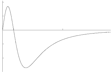
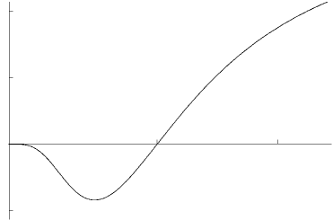
Figure 1: On the right, the heat capacity $C_{\Omega}$ as a function of the temperature $T$ (at a fixed value of $\Omega$) and on the left, the compressibility $\epsilon_{T}$ as a function of the angular velocity $\Omega$ (at a fixed value of $T$) of a five dimensional singly spinning black hole is shown. The heat capacity is positive in the region where $(T/\Omega)\,<\left(2\pi\sqrt{3}\right)^{-1}\simeq 0.092$ (or equivalently for $\nu>0.6$) and the compressibility is positively defined in the region where $(T/\Omega)>\sqrt{3}/(2\pi)\simeq 0.276$ (or for $\nu<0.14$) implying the instability of the black hole in the canonical and grand canonical ensembles. The heat capacity tends to zero when approaching the singular extremal black hole solution with $T=0$.

3.3.2 Black ring

We consider now the dynamical equilibrium condition $\lambda=2\nu/(1+\nu^{2})$ that corresponds to a regular black ring with one angular momentum.

The Gibbs potential can be written as a function of the temperature and the angular velocity as follows

$${\cal G}[T,\Omega]=\frac{\pi}{4G\,\Omega^{2}}\left(1+\sqrt{1+\frac{16\pi^{2}T^{2}}{\Omega^{2}}}\right)^{-1}\,.$$ (42)

A straightforward computation leads to

$$G\Omega^{3}\,C_{\Omega}=\frac{\pi^{2}x\left(1+\sqrt{1+x^{2}}-2x^{2}\sqrt{1+x^{2}}\right)}{\left(1+x^{2}\right)^{3/2}\left(1+\sqrt{1+x^{2}}\right)^{3}}\,,$$ (43)

where $x=4\pi T/\Omega$. It turns out that solutions with $T/\Omega\,<\left(4\pi\sqrt{2/\sqrt{3}}\right)^{-1}\simeq 0.074$ are stable against thermal fluctuations, $C_{\Omega}>0$. It is also important to note that in the extremal limit where $T\rightarrow 0$ or $\nu\rightarrow 1$ the heat capacity goes to zero as shown in Fig. 2. This behavior for the heat capacity is expected and can be drawn from Nernst theorem.

Similarly the compressibility can be computed

$$GT^{4}\,\epsilon_{T}=-\frac{2+3\bar{x}^{2}}{1024\pi^{3}\bar{x}^{3}\left(1+\bar{x}^{2}\right)^{3/2}}\,,$$ (44)

where $\bar{x}=\Omega/(4\pi T)$ and so, for any value of the parameters, it is always negative. Therefore, the black ring is also thermodynamically unstable in the grand-canonical and canonical ensembles.

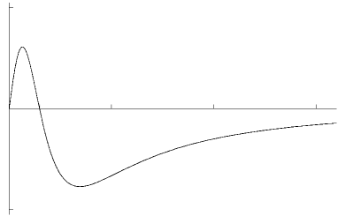
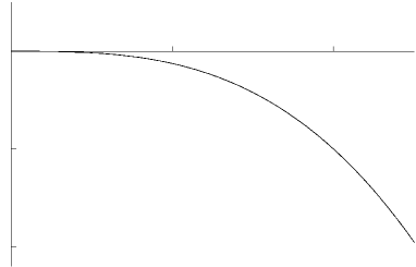
Figure 2: Plot of the heat capacity $C_{\Omega}$ as a function of the temperature $T$ for a given angular velocity (left) and the compressibility $\epsilon_{T}$ as a function of the angular velocity $\Omega$ for a given temperature (right) for a singly spinning black ring. The black ring is unstable in the canonical and grand canonical ensembles: the compressibility is always negative and the heat capacity is only positive when $T/\Omega\,<\left(4\pi\sqrt{2/\sqrt{3}}\right)^{-1}\simeq 0.074$. In the extremal limit ($T=0$) the heat capacity of the black ring is zero.

4 Charged black objects

In this section we compute the stress tensor of charged $5$-dimensional black objects. In particular, we discuss the Reissner-Nordstrom black hole, a supersymmetric black ring solution, and black string solutions in Einstein-Maxwell-dilaton theories. We also obtain the equilibrium condition for the black string solutions that are obtained as limit of black rings in [14].

4.1 Reissner-Nordstrom black hole in five dimensions

As a warm-up exercise, we begin by analyzing the Reissner-Nordstrom black hole. The static black hole solution of Einstein-Maxwell field equations has the following line element

$$ds^{2}=-V(r)\,dt^{2}+\frac{dr^{2}}{V(r)}+r^{2}\,d\Omega^{2}_{3}\,,$$ (45)

where

$$V(r)=1-\frac{m}{r^{2}}+\frac{q^{2}}{r^{4}}\,.$$ (46)

The parameters $(m,q)$ are related to the mass and electric charge respectively. The coordinates range between $0\leq\theta<\pi/2$ and $0\leq\phi,\psi<\pi$.

Using the counterterm method we find the relevant stress energy component

$$\tau_{tt}=\frac{1}{8\pi G}\left(-\frac{3}{2}\,\frac{m}{r^{3}}+\left(\frac{9m^{2}}{8}+\frac{3q^{2}}{2}\right)\,\frac{1}{r^{5}}+\mathcal{O}(1/r^{7})\right)\,.\\$$

As expected, the charge contribution is subleading in the $\tau_{tt}$ component of the stress tensor.

From (5) we can then calculate the conserved mass associated with the closed surface $\Sigma$

$$M\equiv\oint_{\Sigma}d^{3}y\sqrt{\sigma}n^{i}\,\tau_{ij}\,\xi_{t}^{j}=\frac{3\,m}{8\,G}\,,$$

where the the normalized Killing vector associated with the mass is $\xi_{t}=\partial_{t}$, matching the ADM computation.

4.2 The supersymmetric black ring

This is the solution of the bosonic sector of five-dimensional minimal supergravity with an action principle

$$I_{0}=\frac{1}{16\pi G}\int_{M}d^{5}x\left(\sqrt{-g}{\left(R-F^{2}\right)}-\frac{8}{3\sqrt{3}}F\wedge F\wedge A\right)-\frac{1}{8\pi G}\int_{\mathcal{\partial M}}K\sqrt{-h}\,d^{4}x,$$ (47)

and field equations

$$R_{\mu\nu}-\frac{1}{2}Rg_{\mu\nu}=2(F_{\mu\sigma}F^{\sigma}_{\nu}-\frac{1}{4}g_{\mu\nu}F^{2}),$$ (48)

$$D_{\mu}F^{\mu\nu}=\frac{1}{2\sqrt{3}\sqrt{-g}}\epsilon^{\nu\mu\sigma\lambda\tau}F_{\mu\sigma}F_{\lambda\tau},$$ (49)

where $F=dA$.

The line element of the black ring solution is given by [37] (see also [25, 38, 39, 40])

$$ds^{2}=-f^{2}(dt+\omega)^{2}+f^{-1}ds^{2}_{4}\,,$$ (50)

with the flat space metric written in ring coordinates

$$ds^{2}_{4}=\frac{R^{2}}{(x-y)^{2}}\Big{[}\frac{dy^{2}}{y^{2}-1}+(y^{2}-1)d\psi^{2}+\frac{dx^{2}}{1-x^{2}}+(1-x^{2})d\phi^{2}\Big{]}\,.$$ (51)

where

$$f^{-1}=1+\frac{Q-q^{2}}{2R^{2}}(x-y)-\frac{q^{2}}{4R^{2}}(x^{2}-y^{2}),~{}~{}\omega=\omega_{\psi}d\psi+\omega_{\phi}d\phi\,,$$ (52)

and

$$\omega_{\phi} = -\frac{q}{8R^{2}}(1-x^{2})\left[3Q-q^{2}(3+x+y)\right]\,,$$ (53)

$$\omega_{\psi} = \frac{3}{2}q(1+y)+\frac{q}{8R^{2}}(1-y^{2})\left[3Q-q^{2}(3+x+y)\right]\,.$$ (54)

The gauge potential is

$$A=\frac{\sqrt{3}}{2}\left[f\,(dt+\omega)-\frac{q}{2}((1+x)\,d\phi+(1+y)\,d\psi)\right]\,.$$ (55)

The coordinates have ranges $-1\leq x\leq 1$ and $-\infty<y\leq-1$, and $\phi,\psi$ have period $2\pi$. The black ring has an event horizon at $y=-\infty$. $Q$ and $q$ are positive constants, proportional to the net charge and to the dipole charge of the ring, respectively. The electric charge relevant for thermodynamics is ${\cal Q}=\sqrt{3}Q/2$.

The same counterterm approach can be used to compute the asymptotic conserved charges. In this computation, it is convenient to use the $(r,\theta)$ coordinates, defined by (21) with $\alpha=1$. The relevant components of the boundary stress tensor are

$$\tau_{tt} = \frac{1}{8\pi G}\left(-\frac{3Q}{r^{3}}-\frac{5}{3}R^{2}\frac{\cos 2\theta}{r^{3}}+\mathcal{O}(1/r^{5})\right)\,,$$

$$\tau_{t\phi} = \frac{1}{8\pi G}\left(-q(3Q-q^{2})\frac{\cos^{2}\theta}{r^{3}}+\mathcal{O}(1/r^{5})\right)\,,$$

$$\tau_{t\psi} = \frac{1}{8\pi G}\left(-q(6\,R^{2}+3Q-q^{2})\frac{\sin^{2}\theta}{r^{3}}+\mathcal{O}(1/r^{5})\right)\,,$$

$$\tau_{\theta\theta} = \frac{1}{8\pi G}\left(\frac{2}{3}R^{2}\frac{\cos 2\theta}{r}+\mathcal{O}(1/r^{3})\right)\,,$$ (56)

$$\tau_{\phi\phi} = \frac{1}{8\pi G}\left(\frac{2}{3}R^{2}(1+2\cos 2\theta)\frac{\cos^{2}\theta}{r}+\mathcal{O}(1/r^{3})\right)\,,$$

$$\tau_{\psi\psi} = \frac{1}{8\pi G}\left(\frac{2}{3}R^{2}(-1+2\cos 2\theta)\frac{\sin^{2}\theta}{r}+\mathcal{O}(1/r^{3})\right)\,.$$

Therefore, the mass and angular momentum as computed from the counterterms are the same as the ADM values

$$M=\frac{3\pi Q}{4G},~{}~{}J_{\varphi}=\frac{\pi}{8G}q(3Q-q^{2}),~{}~{}J_{\psi}=\frac{\pi}{8G}q(6\,R^{2}+3Q-q^{2})\,.$$

For this supersymmetric solution, the surface gravity and the angular velocities of the event horizon vanish. Despite this, the horizon area is finite and depends on both the global and dipole charges. We present more details on the role of the charges and the thermodynamics of the supersymmetric black ring in the Discussion section.

4.3 Black string and balance condition

In this section we discuss the 5-dimensional charged boosted black string solutions in Einstein-Maxwell-dilaton theory [14] by using the counterterm method. The action is

$$I=\frac{1}{16\pi G}\int d^{5}x\sqrt{-g}\left(R-\frac{1}{2}(\partial\phi)^{2}-\frac{1}{4}e^{-\alpha\phi}F^{2}\right)\,.$$ (57)

It is convenient to express the dilaton coupling as in [14]

$$\alpha^{2}=\frac{4}{N}-\frac{4}{3}\,,\qquad 0<N\leq 3\,.$$ (58)

We will obtain the relevant components of the stress tensor and discuss the balance condition.

The solution, with the boost parameter $\sigma$ and the event horizon $r=r_{0}$, is

$$ds^{2}=-\frac{\hat{f}}{h^{N/3}}\left(dt-\frac{r_{0}\sinh\sigma\cosh\sigma}{r\hat{f}}\,dz\right)^{2}+\frac{f}{h^{N/3}\hat{f}}\,dz^{2}+h^{2N/3}\left(\frac{dr^{2}}{f}+r^{2}d\Omega_{2}^{2}\right)\,,$$ (59)

where the (magnetic) charge is parametrized by $\gamma$.

The gauge potential and the dilaton for the magnetic solution are, respectively,

$$A_{\phi}=\sqrt{N}\,r_{0}\sinh\gamma\cosh\gamma\,(1+\cos\theta)\,,\qquad e^{\phi}=h^{N\alpha/2}\,,$$ (60)

and

$$f=1-\frac{r_{0}}{r}\,,\qquad\hat{f}=1-\frac{r_{0}\cosh^{2}\sigma}{r}\,,\qquad h=1+\frac{r_{0}\sinh^{2}\gamma}{r}\,.$$ (61)

The black string solutions that are obtained as limit of black rings should also satisfy the equilibrium condition. The equilibrium condition is a constraint on the parameters of the unbalanced ring solution (3.1) that is equivalent with the removing of all conical singularities in the metric.

A nice physical interpretation was given in [14]: the absence of conical singularities is equivalent with the equilibrium of the forces acting on the ring. A black ring can be obtained by bending a boosted black string. Thus, the linear velocity along the string becomes the angular velocity of the black ring. The equilibrium of centrifugal and gravitational forces imposes a constraint on the radius of the ring $R$, the mass, and the angular momentum. In this way one can see that, indeed, just two parameters are independent in the solution of the neutral black ring.

Applying the same procedure as before we find that the relevant component of the boundary stress tensor is

$$\tau_{zz}=\frac{1}{8\pi G}\left(\frac{r_{0}^{2}}{2}\left(1-\sinh^{2}{\sigma}+N\sinh^{2}\gamma\right)\frac{1}{r^{2}}+\mathcal{O}(1/r^{3})\right)\,.$$ (62)

From a more general definition of Carter [42], in the absence of external forces the equations of motion of brane-like objects obey $K^{\rho}_{\mu\nu}T^{\mu\nu}=0$, which implies the component of the stress tensor in the z-direction (the pressure) vanishes $T_{zz}=0$.

Thus, asymptotically, this equality (at first order) constrains the values of the boost parameter with the charge (parameterized by $\gamma$) in the following manner

$$\sinh^{2}\sigma=1+N\sinh^{2}\gamma\,,$$ (63)

that is in agreement with the regularity constrains in [14] and the equilibrium condition found in [43] for thin black rings.

By direct integration of the stress energy components the conserved charges, mass and angular momentum, match exactly those from the ADM definition, namely

$$M=\frac{\pi}{8G}\,R\,r_{0}\cosh 2\sigma,\qquad J=-\frac{\pi}{8G}\,R^{2}r_{0}\cosh\sigma\sinh\sigma\,.$$ (64)

5 Discussion

In this paper we systematically have applied the counterterm method for asymptotically flat spacetimes to 5-dimensional black objects. In this way, we have derived various thermodynamic relations for several stationary black objects.

We hope that our unified treatment of black holes, black rings, and black strings with an emphasis on the role of the quasi-Euclidean section for thermodynamics is useful to the reader.

On the Quasi-Euclidean method

The notion of asymptotic flatness of isolated systems is intimately related to the possibility of defining the total stress-energy tensor that characterizes the gravity system [20]. It is well known that a spacetime is asymptotically flat if it is possible to attach to its corresponding manifold a boundary in null directions ($\cal{I}$) — since null rays reach ($\cal{I}$) for an infinite value of their affine parameter, this is called null infinity. Spatial infinity, $\iota^{0}$ (the part of infinity that is reached along spacelike geodesics), is represented by one point in the Penrose diagram of conformal compactification for Minkowski space.

It is important to emphasize that it is also possible to foliate the spacetime with spacelike foliations: spacelike surfaces can be constructed that extend through null infinity. Such surfaces are called hyperboidal as their asymptotic behaviour is similar to standard hyperboloids in Minkowski spacetime. In this context, it is better to visualize $\iota^{0}$ as the hyperboloid of spacelike directions (it is isometric to the unit $4$-dimensional de Sitter space).

From a physical point of view, $\iota^{0}$ can be interpreted as the place where an observer ends up when shifted to larger and larger distances. However, for studying holography in stationary flat spacetimes, it seems more natural to impose boundary conditions at $\iota^{0}$ rather than $\cal{I}$. Therefore, the renormalized ‘boundary’ stress tensor we used in this paper is assigned to spatial infinity $\iota^{0}$ of asymptotically flat spacetimes.

A key point is that one’s intuition about Euclidean sections does not apply to black rings — there is no real non-singular Euclidean section in this case. Therefore, a black ring should be described by a complex Euclidean geometry [27] and its associated real action (‘thermodynamic action’).

Consequently we employed the quasi-Euclidean method [6, 29], which was applied to black rings for the first time in [13]. The properties of the black ring interior become encoded in a set of conditions at the ‘bolt’ of the complex geometry. Thus, the partition function computed as a functional integral is extremized by a certain stationary complex black ring metric.

A natural question that arises is if the physical system described by this partition function is a real Lorentzian black ring. The answer is yes, precisely because the stress tensors for the complex black ring and for the related Lorentzian black ring coincide. For example, in the zero loop approximation, the expectation value of energy from the partition function will coincide with the energy of the complex black ring calculated from the boundary stress-tensor; in turn, the latter characterizes the energy of the real Lorentzian black ring.

Further support for using quasi-Euclidean instantons to construct gravitational partition functions was given in [36]. In this work, the authors discuss the thermodynamic instabilities of several spinning black objects in the grand-canonical ensemble. They found that the partition functions of neutral spinning black holes and black rings in flat spacetime possess negative modes at the perturbative level.

A central result in our work is the computation of the renormalized action (31) on the quasi-Euclidean section. The black ring solutions have been shown to satisfy the first law of black hole mechanics, thus suggesting that their entropy is one quarter of the event horizon area. We have made this more precise by computing the gravitational action to check the quantum statistical relation as well as the first law of thermodynamics. Our computation can be considered as an independent check that the entropy/area relation applies also for the black rings.

On the thermodynamics

The thermodynamics of black rings in different ensembles has been previously presented in the literature [13, 30, 36]. For completeness, we also present a discussion of thermodynamic stability within quasilocal formalism.

Four-dimensional black holes are highly constrained objects. That is, an isolated electrovac black hole can be characterized, uniquely and completely, by just three macroscopic parameters: its mass, angular momentum, and charge. Thus, all multipole moments of the gravitational field are radiated away in the collapse to a black hole, except the monopole and dipole moments [44] — they cannot be radiated away because the graviton has spin $2$.

There are no black objects with an electric dipole in four dimensions. The black holes have ‘smooth’ horizons (there are no ripples or higher multipoles) and are classically stable. Moreover, for asymptotically flat solutions, the event horizons of non-spherical topology are forbidden.

For vacuum Einstein gravity in more than four dimensions there is no uniqueness since a richer range of regular black objects inhabit the space. These include not just black holes [23] with spherical $S^{D-2}$ horizon geometry, but also black rings [43] with $S^{1}\times S^{D-3}$ and blackfolds [46] with topological, i.e. $S^{p+2}\times S^{D-p-4}$ when $p\leq D-7$, horizon geometries.

Many studies on the thermodynamics (some reviews [25, 48, 49, 50]), ergoregions [47], and combinations of black objects leading to more sophisticated solutions [51] uphold the exciting richness of black objects. And moreover, as we present here, new insights into the thermodynamics remain to be unveiled. Perhaps because of the tight contact with string theory, the most widely employed scheme to explore the thermodynamics of black holes in five [24, 45] and higher space-time dimensions [43] seems to be the microcanonical ensemble.

In this paper, to study the stability of five dimensional black holes, we have carried out the thermodynamic analysis mainly in the canonical and grand canonical ensembles. Not only the thermodynamic stability but also the phase structure depends on the chosen ensemble.

Already in our case, of the canonical $f$ vs $t$ and grand canonical $g$ vs $t$ ensembles, some significant differences can directly be noticed from the structure of these phase diagrams for the black hole (dashed line) and the black ring (solid line) in Fig. 3.

The single phases, one for each, of the black hole and ring in the grand-canonical ensemble contrast the three phases, two for the black hole and a single one for the black ring, of the canonical ensemble. The entropy $S[M,\Omega]=A/(4\,G)$ and the enthalpy, $H[M,\Omega]=M-\Omega\,J$ are also shown for comparison. For a fixed mass, in the microcanonical ensemble a swallowtail structure is found for the two black ring phases with a single phase for the black hole. Leaving the mass fixed, yet a different structure is found: for the $h$ vs $\omega$ each of the single black hole and black ring phases join at a maximum value of the angular velocity. The plots we present here are new although the discussions comparing the different structures of the phase diagrams can also be found in [30].

                             

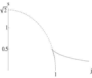
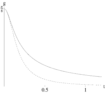
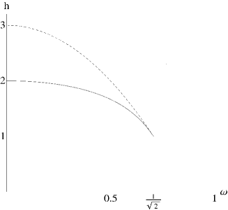
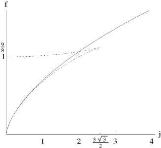
Figure 3: The phase diagrams of a singly spinning black hole (dashed) and a black ring (solid) in different thermodynamic ensembles: (a) microcanonical, (b) enthalpy, (c) grand canonical and (d) canonical.

On the nature of charges

Another case where the classical uniqueness results do not apply is for gravity theories with scalar fields non-minimally coupled to gauge fields. Due to the non-minimal coupling, a black hole solution in Einstein-Maxwell-dilaton gravity can carry also a scalar charge and the first law gets modified [52].

The scalar charge is not protected by a gauge symmetry and so it is not conserved. Since it depends on the other conserved charges it does not represent, though, a new quantum number associated with the black hole — this kind of charge is called secondary hair. Furthermore, this charge is not localized and exists outside the horizon.

In Section $4$ we studied a supersymmetric ring solution in minimal supergravity. Since it is an extremal black object a computation of the action is not possible (the periodicity of the ‘Euclidean time’ cannot be fixed). However, one can compute the entropy by using the entropy function formalism for spinning extremal black holes [54].

Due to the attractor mechanism the entropy does not depend on scalar charges, but it depends on both, the global charge and the dipole. Since the dipole is a non-conserved charge, one may be tempted to make an analogy with the scalar charge. However, there is an important difference: unlike the scalar charge, the dipole charge is a localized charge. Thus, it can be measured by flux integrals on surfaces linked to the black ring’s horizon [14] and has a microscopic interpretation (brane wrapping contractible cycles of CY).

One important question emerges: what is the interpretation of the dipole within the quasilocal formalism? In other words, can an asymptotic observer distinguish between a black hole or a black ring with the same conserved charges? The answer is obviously yes: analogous to an electric dipole whose moments can be read off from a multipole expansion at infinity, the subleading terms in the boundary stress tensor should encode the information necessarily to distinguish between black objects with different horizon topologies in the bulk.

There is, though, another subtlety we would like to discuss in detail now. Due to the existence of the Chern-Simons interaction in the Lagrangian, the equation of motion for the gauge field is modified. Therefore, the topological density of gauge field itself becomes the source of electric charge. Consequently, even if it is conserved, the usual Maxwell charge of a black ring seems to be diffusely distributed throughout the spacetime. Thus, the ‘Maxwell charge’ in this case is gauge invariant and conserved but not localized.

The resolution of this problem was provided in [55, 56]: the correct charges that appear in the entropy are the ‘Page charges’. These charges are conserved and localized but not gauge invariant (see [57, 58] for a discussion of different kinds of charges). It was shown in [55] that once the entropy function is expressed in terms of these physical 5-dimensional charges it becomes manifestly gauge invariant (due to a spectral flow symmetry of the theory).

The near horizon geometry of a black hole should capture the complete information about its microscopic degeneracy. However, if a black hole does have ‘hair’ (degrees of freedom living outside the horizon), there are subtle distinctions between the asymptotic charges and the charges entering in the CFT [59].

In the case of the susy black ring, one angular momentum is generated by degrees of freedom living outside the horizon in the form of crossed electric and magnetic supergravity fields [38, 60].

However, for the supersymmetric black ring the microscopic angular momentum density is not equal to the angular momentum at infinity. Interestingly enough, the ‘Page’ angular momentum [56] is in fact the intrinsic angular momentum of the susy black ring and our arguments support the point of view in [61].

While our discussion has focussed on stationary solutions, it will be interesting to investigate whether similar methods can be useful as well for studying the time-dependent backgrounds given in [62]. These solutions are obtained by a simple analytic continuation of a black hole geometry. At a first look, it seems that the stress tensor of these time dependent solutions should be somehow related to the stress tensor of the ‘seed’ black hole solution. However, this case is more subtle since the energy-momentum carried away by gravitational radiation is associated to null infinity.

Finally, we want to mention that the counterterm method can be also useful in investigating the thermodynamics of the black rings obtained in [63] (e.g., [64]).

References

- [1] R. B. Mann, “Expanding the Area of Gravitational Entropy,” Found. Phys. 33, 65 (2003) [arXiv:gr-qc/0211047].
- [2] G. W. Gibbons and S. W. Hawking, “Action Integrals And Partition Functions In Quantum Gravity,” Phys. Rev. D 15, 2752 (1977).
- [3] J. D. Brown and J. W. . York, “Quasilocal energy and conserved charges derived from the gravitational action,” Phys. Rev. D 47, 1407 (1993) [arXiv:gr-qc/9209012].
- [4] J.D. Brown, J. Creighton and R.B. Mann, “Temperature, Energy and Heat Capacity of Asymptotically Anti-de Sitter Black Holes,” Phys. Rev. D50 6394 (1994). [arXiv:gr-qc/9405007].
- [5] J. D. E. Creighton and R. B. Mann, “Quasilocal thermodynamics of dilaton gravity coupled to gauge fields,” Phys. Rev. D 52, 4569 (1995) [arXiv:gr-qc/9505007].
- [6] I. S. Booth and R. B. Mann, “Moving observers, non-orthogonal boundaries, and quasilocal energy,” Phys. Rev. D 59, 064021 (1999) [arXiv:gr-qc/9810009].
- [7] S. R. Lau, “Lightcone reference for total gravitational energy,” Phys. Rev. D 60, 104034 (1999) [arXiv:gr-qc/9903038].
- [8] R. B. Mann, “Misner string entropy,” Phys. Rev. D 60, 104047 (1999) [arXiv:hep-th/9903229].
- [9] P. Kraus, F. Larsen and R. Siebelink, “The gravitational action in asymptotically AdS and flat spacetimes,” Nucl. Phys. B 563, 259 (1999) [arXiv:hep-th/9906127].
-
[10]
M. Henningson and K. Skenderis,
“The holographic Weyl anomaly,”
JHEP 9807, 023 (1998)
[arXiv:hep-th/9806087];
V. Balasubramanian and P. Kraus, “A stress tensor for anti-de Sitter gravity,” Commun. Math. Phys. 208, 413 (1999) [arXiv:hep-th/9902121];
K. Skenderis and S. N. Solodukhin, “Quantum effective action from the AdS/CFT correspondence,” Phys. Lett. B 472, 316 (2000) [arXiv:hep-th/9910023];
M. Bianchi, D. Z. Freedman and K. Skenderis, “How to go with an RG flow,” JHEP 0108, 041 (2001) [arXiv:hep-th/0105276];
K. Skenderis, “Lecture notes on holographic renormalization,” Class. Quant. Grav. 19, 5849 (2002) [arXiv:hep-th/0209067];
S. de Haro, S. N. Solodukhin and K. Skenderis, “Holographic reconstruction of spacetime and renormalization in the AdS/CFT correspondence,” Commun. Math. Phys. 217, 595 (2001) [arXiv:hep-th/0002230];
K. Skenderis, “Asymptotically anti-de Sitter spacetimes and their stress energy tensor,” Int. J. Mod. Phys. A 16, 740 (2001) [arXiv:hep-th/0010138];
M. Bianchi, D. Z. Freedman and K. Skenderis, “Holographic renormalization,” Nucl. Phys. B 631, 159 (2002) [arXiv:hep-th/0112119]. - [11] D. Astefanesei, N. Banerjee and S. Dutta, “(Un)attractor black holes in higher derivative AdS gravity,” JHEP 0811, 070 (2008) [arXiv:0806.1334 [hep-th]].
- [12] R. G. Cai and N. Ohta, “Surface counterterms and boundary stress-energy tensors for asymptotically non-anti-de Sitter spaces,” Phys. Rev. D 62, 024006 (2000) [arXiv:hep-th/9912013].
- [13] D. Astefanesei and E. Radu, “Quasilocal formalism and black ring thermodynamics,” Phys. Rev. D 73, 044014 (2006) [arXiv:hep-th/0509144].
- [14] R. Emparan, “Rotating circular strings, and infinite non-uniqueness of black rings,” JHEP 0403, 064 (2004) [arXiv:hep-th/0402149].
- [15] D. Marolf, “Asymptotic flatness, little string theory, and holography,” JHEP 0703, 122 (2007) [arXiv:hep-th/0612012].
- [16] R. B. Mann and D. Marolf, “Holographic renormalization of asymptotically flat spacetimes,” Class. Quant. Grav. 23, 2927 (2006) [arXiv:hep-th/0511096].
- [17] R. B. Mann, D. Marolf and A. Virmani, “Covariant counterterms and conserved charges in asymptotically flat spacetimes,” Class. Quant. Grav. 23, 6357 (2006) [arXiv:gr-qc/0607041].
- [18] D. Astefanesei, R. B. Mann and C. Stelea, “Note on counterterms in asymptotically flat spacetimes,” Phys. Rev. D 75, 024007 (2007) [arXiv:hep-th/0608037].
- [19] T. Liko and D. Sloan, “First-order action and Euclidean quantum gravity,” Class. Quant. Grav. 26, 145004 (2009) [arXiv:0810.0297 [gr-qc]].
- [20] R. L. Arnowitt, S. Deser and C. W. Misner, “The dynamics of general relativity,” arXiv:gr-qc/0405109.
- [21] D. Baskaran, S. R. Lau and A. N. Petrov, “Center of mass integral in canonical general relativity,” Annals Phys. 307, 90 (2003) [arXiv:gr-qc/0301069].
- [22] G. W. Gibbons, D. Ida and T. Shiromizu, “Uniqueness and non-uniqueness of static black holes in higher dimensions,” Phys. Rev. Lett. 89, 041101 (2002) [arXiv:hep-th/0206049].
- [23] R. C. Myers and M. J. Perry, “Black Holes In Higher Dimensional Space-Times,” Annals Phys. 172, 304 (1986).
- [24] R. Emparan and H. S. Reall, “A rotating black ring in five dimensions,” Phys. Rev. Lett. 88, 101101 (2002) [arXiv:hep-th/0110260].
- [25] R. Emparan and H. S. Reall, “Black rings,” Class. Quant. Grav. 23, R169 (2006) [arXiv:hep-th/0608012].
- [26] J. D. Brown, E. A. Martinez and J. W. . York, “Rotating Black Holes, Complex Geometry, And Thermodynamics,” Annals N. Y. Acad. Sci. 631, 225 (1991).
- [27] J. D. Brown, E. A. Martinez and J. W. . York, “Complex Kerr-Newman geometry and black hole thermodynamics,” Phys. Rev. Lett. 66, 2281 (1991).
- [28] K.C.K. Chan, J.D.E. Creighton, and R.B. Mann, “Conserved masses in GHS Einstein and String Black Holes and Consistent Thermodynamics,” Phys. Rev. D54, 3892 (1996).
- [29] I. S. Booth and R. B. Mann, “Complex instantons and charged rotating black hole pair creation,” Phys. Rev. Lett. 81, 5052 (1998) [arXiv:gr-qc/9806015].
- [30] H. Elvang, R. Emparan and A. Virmani, “Dynamics and stability of black rings,” JHEP 0612, 074 (2006) [arXiv:hep-th/0608076].
- [31] S. Hollands, A. Ishibashi and R. M. Wald, “A Higher Dimensional Stationary Rotating Black Hole Must be Axisymmetric,” Commun. Math. Phys. 271, 699 (2007) [arXiv:gr-qc/0605106].
- [32] D. Astefanesei and H. Yavartanoo, “Stationary black holes and attractor mechanism,” Nucl. Phys. B 794, 13 (2008) [arXiv:0706.1847 [hep-th]].
- [33] H. Elvang and R. Emparan, “Black rings, supertubes, and a stringy resolution of black hole non-uniqueness,” JHEP 0311 (2003) 035 [arXiv:hep-th/0310008].
- [34] S. Tomizawa, Y. Yasui and A. Ishibashi, “A uniqueness theorem for charged rotating black holes in five-dimensional minimal supergravity,” Phys. Rev. D 79, 124023 (2009) [arXiv:0901.4724 [hep-th]].
- [35] Herbert B. Callen, “Thermodynamics and introduction to thermostatics”, John Wiley and Sons (1985).
- [36] R. Monteiro, M. J. Perry and J. E. Santos, “Thermodynamic instability of rotating black holes,” Phys. Rev. D 80, 024041 (2009) [arXiv:0903.3256 [gr-qc]].
- [37] H. Elvang, R. Emparan, D. Mateos and H. S. Reall, “A supersymmetric black ring,” Phys. Rev. Lett. 93, 211302 (2004) [arXiv:hep-th/0407065].
- [38] H. Elvang, R. Emparan, D. Mateos and H. S. Reall, “Supersymmetric black rings and three-charge supertubes,” Phys. Rev. D 71, 024033 (2005) [arXiv:hep-th/0408120].
- [39] I. Bena and N. P. Warner, “One ring to rule them all … and in the darkness bind them?,” Adv. Theor. Math. Phys. 9, 667 (2005) [arXiv:hep-th/0408106].
- [40] I. Bena and N. P. Warner, “Black holes, black rings and their microstates,” Lect. Notes Phys. 755, 1 (2008) [arXiv:hep-th/0701216].
- [41] D. Astefanesei, M. J. Rodriguez and S. Theisen, “Quasilocal equilibrium condition for black ring,” JHEP 0912, 040 (2009) [arXiv:0909.0008 [hep-th]].
- [42] B. Carter, “Essentials of classical brane dynamics,” Int. J. Theor. Phys. 40, 2099 (2001) [arXiv:gr-qc/0012036].
- [43] R. Emparan, T. Harmark, V. Niarchos, N. A. Obers and M. J. Rodriguez, “The Phase Structure of Higher-Dimensional Black Rings and Black Holes,” JHEP 0710, 110 (2007) [arXiv:0708.2181 [hep-th]].
- [44] P. K. Townsend, “Black holes,” arXiv:gr-qc/9707012.
- [45] H. Elvang, R. Emparan and P. Figueras, “Phases of Five-Dimensional Black Holes,” JHEP 0705, 056 (2007) [arXiv:hep-th/0702111].
- [46] R. Emparan, T. Harmark, V. Niarchos and N. A. Obers, “Blackfolds,” Phys. Rev. Lett. 102, 191301 (2009) [arXiv:0902.0427 [hep-th]].
-
[47]
H. Elvang, P. Figueras, G. T. Horowitz, V. E. Hubeny and M. Rangamani,
“On Universality of Ergoregion Mergers,”
Class. Quant. Grav. 26, 085011 (2009)
[arXiv:0810.2778 [gr-qc]];
M. Durkee, “Geodesics and Symmetries of Doubly-Spinning Black Rings,” Class. Quant. Grav. 26, 085016 (2009) [arXiv:0812.0235 [gr-qc]]. - [48] R. Emparan and H. S. Reall, “Black Holes in Higher Dimensions,” Living Rev. Rel. 11, 6 (2008) [arXiv:0801.3471 [hep-th]].
- [49] N. A. Obers, “Black Holes in Higher-Dimensional Gravity,” Lect. Notes Phys. 769, 211 (2009) [arXiv:0802.0519 [hep-th]].
- [50] B. Kleihaus, J. Kunz and F. Navarro-Lerida, “Rotating Black Holes in Higher Dimensions,” AIP Conf. Proc. 977, 94 (2008) [arXiv:0710.2291 [hep-th]].
-
[51]
H. Iguchi and T. Mishima,
“Black di-ring and infinite nonuniqueness,”
Phys. Rev. D 75, 064018 (2007)
[Erratum-ibid. D 78, 069903 (2008)]
[arXiv:hep-th/0701043];
J. Evslin and C. Krishnan, “The Black Di-Ring: An Inverse Scattering Construction,” Class. Quant. Grav. 26, 125018 (2009) [arXiv:0706.1231 [hep-th]];
H. Elvang and P. Figueras, “Black Saturn,” JHEP 0705 (2007) 050 [arXiv:hep-th/0701035];
H. Elvang and M. J. Rodriguez, “Bicycling Black Rings,” JHEP 0804, 045 (2008) [arXiv:0712.2425 [hep-th]]. - [52] G. W. Gibbons, R. Kallosh and B. Kol, “Moduli, scalar charges, and the first law of black hole thermodynamics,” Phys. Rev. Lett. 77, 4992 (1996) [arXiv:hep-th/9607108].
- [53] D. Astefanesei, K. Goldstein and S. Mahapatra, “Moduli and (un)attractor black hole thermodynamics,” Gen. Rel. Grav. 40, 2069 (2008) [arXiv:hep-th/0611140].
- [54] D. Astefanesei, K. Goldstein, R. P. Jena, A. Sen and S. P. Trivedi, “Rotating attractors,” JHEP 0610, 058 (2006) [arXiv:hep-th/0606244].
- [55] X. D. Arsiwalla, “Entropy Functions with 5D Chern-Simons terms,” arXiv:0807.2246 [hep-th].
- [56] K. Hanaki, K. Ohashi and Y. Tachikawa, “Comments on charges and near-horizon data of black rings,” JHEP 0712, 057 (2007) [arXiv:0704.1819 [hep-th]].
- [57] D. Marolf, “Chern-Simons terms and the three notions of charge,” arXiv:hep-th/0006117.
- [58] G. Compere, K. Copsey, S. de Buyl and R. B. Mann, “Solitons in Five Dimensional Minimal Supergravity: Local Charge, Exotic Ergoregions, and Violations of the BPS Bound,” arXiv:0909.3289 [hep-th].
-
[59]
N. Banerjee, I. Mandal and A. Sen,
“Black Hole Hair Removal,”
JHEP 0907, 091 (2009)
[arXiv:0901.0359 [hep-th]];
D. P. Jatkar, A. Sen and Y. K. Srivastava, “Black Hole Hair Removal: Non-linear Analysis,” arXiv:0907.0593 [hep-th]. - [60] I. Bena, C. W. Wang and N. P. Warner, “Sliding rings and spinning holes,” JHEP 0605, 075 (2006) [arXiv:hep-th/0512157].
- [61] I. Bena and P. Kraus, “Microscopic description of black rings in AdS/CFT,” JHEP 0412, 070 (2004) [arXiv:hep-th/0408186].
-
[62]
G. Tasinato, I. Zavala, C. P. Burgess and F. Quevedo,
“Regular S-brane backgrounds,”
JHEP 0404, 038 (2004)
[arXiv:hep-th/0403156];
D. Astefanesei and G. C. Jones, “S-branes and (anti-)bubbles in (A)dS space,” JHEP 0506, 037 (2005) [arXiv:hep-th/0502162];
A. Kaya, “Supergravity solutions for harmonic, static and flux S-branes,” JHEP 0605, 058 (2006) [arXiv:hep-th/0601202];
V. Baukh and A. Zhuk, “Sp-brane accelerating cosmologies,” Phys. Rev. D 73, 104016 (2006) [arXiv:hep-th/0601205]. -
[63]
S. S. Yazadjiev,
“Rotating non-asymptotically flat black rings in charged dilaton gravity,”
Phys. Rev. D 72, 104014 (2005)
[arXiv:hep-th/0511016];
S. S. Yazadjiev, “Solution generating in 5D Einstein-Maxwell-dilaton gravity and derivation of dipole black ring solutions,” JHEP 0607, 036 (2006) [arXiv:hep-th/0604140];
A. A. Pomeransky and R. A. Sen’kov, “Black ring with two angular momenta,” arXiv:hep-th/0612005. - [64] D. Astefanesei, M. J. Rodriguez and S. Theisen, “Thermodynamic instability of doubly spinning black objects,” arXiv:1003.2421 [hep-th].