Study of NGC 5128 Globular Clusters Under Multivariate Statistical Paradigm

Abstract

An objective classification of the globular clusters of NGC 5128 has been carried out by using a model-based approach of cluster analysis. The set of observable parameters includes structural parameters, spectroscopically determined Lick indices and radial velocities from the literature. The optimum set of parameters for this type of analysis is selected through a modified technique of Principal Component Analysis, which differs from the classical one in the sense that it takes into consideration the effects of outliers present in the data. Then a mixture model based approach has been used to classify the globular clusters into groups. The efficiency of the techniques used is tested through the comparison of the misclassification probabilities with those obtained using the K-means clustering technique. On the basis of the above classification scheme three coherent groups of globular clusters have been found. We propose that the clusters of one group originated in the original cluster formation event that coincided with the formation of the elliptical galaxy, and that the clusters of the two other groups are of external origin, from tidally stripped dwarf galaxies on random orbits around NGC 5128 for one group, and from an accreted spiral galaxy for the other.

1 Introduction

Globular Clusters (GCs) are touchstones of astrophysics. Their study addresses many important issues ranging from stellar evolution to the formation of galaxies and cosmology. However their origin and formation history, which are obviously linked to that of their parent galaxy, are still poorly understood.

Classical formation of galaxies can be divided into five major categories: (i) the monolithic collapse model,(ii) the major merger model, (iii) the multiphase dissipational collapse model (iv) the dissipationless merger model and (v) accretion and in situ hierarchical merging.

According to the monolithic collapse model an elliptical galaxy is formed through the collapse of an isolated massive gas cloud at high redshift (Larson 1975; Carlberg 1984; Arimato & Yoshi 1987). In this model the color distribution of GCs is unimodal and the rotation of GCs is produced by the tidal force from satellite galaxies (Peebles 1969). In the major merger model elliptical galaxies are formed by the merger of two or more disk galaxies (Toomre 1977; Ashman & Zepf 1992; Zepf et al. 2000). Younger GCs are formed out of the shocked gas in the disk while blue GCs come from the halos of the merging galaxies (Bekki et al. 2002). As a result the color distribution is bimodal. In this scenario, the kinematic properties of the GCs depend weakly on the orbital configuration of the merging galaxies, but the metal-rich GCs are generally located in the inner region of the galaxy, and the metal-poor ones in the outer regions.

The multiphase dissipational collapse has been proposed by Forbes et al. (1997). According to this model the GCs form in distinct star formation episodes through dissipational collapse. In addition there is tidal stripping of GCs from satellite dwarf galaxies. Blue (metal-poor) GCs form in the initial phase and red (metal-rich) GCs form from the enriched medium at a later epoch, thus producing a bimodal color distribution of the GCs. This model predicts that the system of blue GCs has no rotation and a high velocity dispersion while the red GCs show some rotation depending on the degree of dissipation. Côté et al. (1998) proposed a model in which the GC color bimodality is due to the capture of metal-poor GCs through merger or tidal stripping. The metal-rich GCs are the initial population of GCs in the galaxy and are more centrally concentrated than the captured GCs. The main difference with the previous model is that no age difference is expected between the blue and red GC populations. The very different origins for the two populations imply rather different orbital properties, in particular the metal-poor GCs should show a larger velocity dispersion than the metal-rich ones, comparable in the outer region to that of the neighboring galaxies.

From the above discussion it appears that there are kinematic differences among the sub populations of GCs in different galaxies. These differences can be used as an observational constraint on the galaxy formation model. In the above studies the GCs are classified as metal-rich and metal-poor on the basis of the value of a single parameter [Fe/H] $>$ or $<$ -1 which is subjective in nature and also inappropriate in a multivariate setup. Concentrating on a single parameter means that one ignores the joint effect of several parameters.

With the above objective in mind we have carried out a multivariate analysis of extragalactic GCs. In this context, NGC 5128 is of interest because it is the nearest giant elliptical galaxy whose large sample of GCs is amenable to spectroscopic observations (Beasley et al. 2008) and whose structural parameters have been derived by fitting models to surface brightness profiles based on HST/ACS imaging (McLaughlin et al. 2008). Also the radial velocities are available for a large subsample of GCs (Woodley et al. 2007).

In the present study we have first used a modified technique of principal component analysis (PCA) (Salibián-Barrera et al. 2006) to search for the optimum set of parameters which gives the maximum variation for the GCs in NGC 5128. This method helps to extract the significant parameters from the large set of photometric, structural, and kinematic parameters. Then we have classified the GCs on the basis of these significant parameters using a model-based method of Cluster Analysis (CA) (Qui & Tamhane 2007) which finds the structure of the optimum groups of GCs instead of choosing groups in an ad hoc manner on the basis of a single parameter. This multivariate analysis helps to enunciate a more efficient theory of GC formation.

In this context it should be mentioned that kinematic studies of GCs in several giant elliptical galaxies show results which differ from galaxy to galaxy (Woodley et al. 2007). In a recent study (Hwang et al. 2008) the rotation of metal-poor and metal-rich GCs have been studied in 6 giant elliptical galaxies, two systems of GCs show strong rotation while the other ones show moderate or weak rotation. We have studied NGC 5128 as the representative of the latter group while it remains important to study representatives of the former group in a multivariate setup, once the adequate data are available.

In this paper the different data sets used are presented in section 2. Section 3 gives a list of the different methods used in the present study while the determination of spectroscopic ages and metallicities is discussed in section 4. The results and discussions are presented in section 5. Brief discussions of the methods used are given in the appendices.

2 Data Set

Our analysis is based on the sample of GCs of the early-type central giant elliptical galaxy in the Centaurus group, NGC 5128, whose structural parameters have been derived by fitting King and Wilson models to the surface brightness profiles based on HST/ACS imaging in the F606W bandpass (McLaughlin et al. 2008). The distance is that adopted by McLaughlin et al. (2008), namely 3.8 Mpc. The sample consists of 130 GCs (3 outliers have been excluded during cluster analysis) whose available structural and photometric parameters are tidal radius ($R_{tid}$, in pc), core radius ($R_{c}$, in pc), half-light radius ($r_{h}$, in pc), central volume density (log$\rho_{0}$, in $M_{\odot}$ p$c^{-3}$), predicted line of sight velocity dispersion at the cluster center ($\sigma_{p,0}$ in km$s^{-1}$), two-body relaxation time at the model projected half-mass radius ($t_{rh}$, in years), galactocentric radius ($R_{gc}$, in kpc), concentration (c$\sim$ log($R_{tid}$/$R_{c}$)), dimensionless central potential of the best fitting model ($W_{0}$), extinction-corrected central surface brightness in the F606W bandpass ($\mu_{0}$ in mag arcsec^-2), V surface brightness averaged over $r_{h}$ ($<\mu_{v}>_{h}$) in mag arcsec^-2, integrated model mass (log$M_{tot}$, in $M_{\odot}$), Washington $T_{1}$ magnitude, extinction corrected color $(C-T_{1})_{0}$ and metallicity ([Fe/H],in dex) determined from the color $(C-T_{1})_{0}$.

The radial velocities ($V_{r}$, in km$s^{-1}$) are available for 48 GCs (Woodley et al. 2007), the position angles ($\psi$, east of north) were derived from the coordinates. There are 51 GCs in common with the sample of GCs observed by Beasley et al. (2008) and the present sample. Among these 21 GCs have published Lick Indices (Beasley et al. 2008). These data are used to derive the ages and metallicities ([Z/H]) of 21 GCs of our sample.

The entire data set of 130 GCs with all the parameters (from the literature as well as derived by authors) are listed in Tables 1 and 2 together with their group membership as a result of CA. The three outliers which have not been considered in the final CA study are marked.

3 Method

In the present work we have used some statistical techniques already developed for proper analysis of the data.

We have considered a robust principal component analysis based on multivariate MM-estimators (Salibián-Barrera et al.2006). Principal Component Analysis is a very common technique used in data reduction and interpretation in multivariate analysis. The above mentioned method has been developed to incorporate robustness property into the classical PCA in order to estimate the effects of outliers present in the data. In this method one MM-estimator of scatter is used instead of sample covariances which are very much sensitive to outliers. In particular the eigenvectors and eigenvalues of multivariate MM-estimators of shape are used as introduced by Tatsuoka & Tyler (2000).

For Cluster Analysis we have used two methods : one is based on Mixture Models and the other is a partitioning method. The mixture model method provides a parametric approach to the clustering problem proposed by Qui & Tamhane (2007). Here the Expectation-Maximization (EM) algorithm is used to compute the maximum likelihood estimators (MLEs) of the parameters of the model. These parameters include mixing proportions, which may be thought of as the prior probabilities of different clusters; then the maximum posterior (Bayes) rule for clustering has been used.

The partitioning method, known as K-means algorithm, is one of the most popular method of clustering developed by MacQueen(1967). This method is distribution-free in nature, but cannot provide any estimate of misclassification error probabilities of observations. Qui & Tamhane (2007) proved that the mixture model method is a better method of clustering since it yields smaller expected misclassification rates. To find the optimum number of clusters (i.e. the value of K) we have used the method developed by Sugar & James (2003).

In the present work we have also used the Levenberg-Marquardt algorithm to compute the rotation amplitudes and position angles of the axes of rotation of different groups obtained from cluster analysis. They are listed in last two columns at the beginning of each group of Table 2 as well as in Table 4.

All the above mentioned methods are discussed in brief in the appendices.

4 Determination of ages and metallicities

We took advantage of the method of Lick indices (Faber 1973, Worthey et al. 1994) to disentangle effects of age and metallicity on integrated spectra of globular clusters. A three-dimensional interpolation and $\chi^{2}$ minimization routine by Sharina, Afanasiev & Puzia (2006) (see also Sharina & Davoust, 2009) allowed us to estimate age, [Z/H], and alpha-element ratio for each individual GC simultaneously. It minimizes the summed difference over all Lick indices between the observational and theoretical index values, weighed by the errors of index measurements. The theoretical Lick indices were obtained using linear interpolation on the grids of Simple Stellar Population models of Thomas et al. (2003, 2004). The errors on the evolutionary parameters depend on the errors of Lick indices and on the accuracy of the radial velocities. The random errors of Lick index measurement in individual spectra depend primarily on the S/N ratio in the spectra. The typical source of systematic errors of Lick indices is quality of calibrations of an instrumental system into the Lick standard one (Worthey et al. 1994).

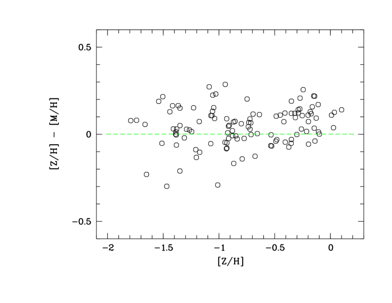
Figure 1: Comparison of the metallicities ([Z/H]) derived by the present method with those of ([M/H]) derived by Beasley et al. (2008)

The comparison of our new metallicity determinations for the entire data set of GCs from Beasley et al. (2008), based on their published Lick indices, with metallicities from Beasley et al. show a very good correlation (r $\simeq$ 0.9; Fig. 1). The photometric metallicities are available for all the GCs of our sample.

5 Results and discussions

5.1 Analysis based on PCA

In PCA our goal is to reduce the large number of parameters in a data set to a minimum number while retaining a maximum variation among the objects (here GCs) under consideration. The technique therefore helps to sort out the optimum set of parameters that causes the maximum overall variation in the nature of GCs in NGC 5128. We initially excluded the observations corresponding to C177 because the values of $R_{tid}$,$r_{h}$ and $<\mu_{v}>_{h}$ for this GC are significantly higher than those of all other GCs. We started with the parameters $R_{tid}$, $R_{c}$, $r_{h}$, log$\rho_{0}$, $\sigma_{p,0}$, $t_{rh}$, $R_{gc}$, c, $W_{0}$, $\mu_{0}$, $<\mu_{v}>_{h}$, log$M_{tot}$, $T_{1}$, $(C-T_{1})_{0}$ and [Fe/H] of 130 GCs and considered only a smaller set of parameters (selected by trial and error of all possible combinations of parameters). We determined the minimum number of principal components on the basis of maximum percentage (90%) of total variation. Since the total set of all possible combinations is very large only a few of the combinations of parameter sets are given for the comparison in Table 3. We mention only these combinations in Table 3 because for all the other combinations the number of principal components to be preserved is higher.

Table 3 shows that sets S3, S4, S6 and S7 have a minimum number of principal components (viz. 1). Among these S7 has the maximum variation corresponding to the first principal component. So S7 has been selected as the optimum set. The parameters found in S7 are the same as those used by Pasquato & Bertin (2008) and Djorgovski (1995) in constituting the fundamental plane (FP) for half-light parameters of GCs in the Galaxy. The present set is different from the FP found by McLaughlin (2000) and McLaughlin & van der Marel (2005) which includes luminosity (L), core mass- to-light ratio ($\gamma_{V,0}$), binding energy ($E_{b}$) and central concentration (c).

5.2 Analysis based on Cluster Analysis

Cluster analysis is the classification of objects into different groups or more precisely the partitioning of a data set into subsets (clusters) so that the data in subsets share some common trait according to some distance measure.

In the previous section the most significant parameters were filtered from a large number (here 15) of parameter sets through the modified PCA which starts from the matrix containing measures of shape parameters involved instead of considering the correlation matrix as is generally done. The most significant parameters responsible for the maximum variation, while keeping the number of principal components minimum are ($<\mu_{v}>_{h},r_{h},\sigma_{p,0}$).

Next the cluster analysis based on the mixture model method is carried out with respect to these three parameters. The optimum number of groups is selected objectively by a widely used method, K-means clustering (MacQueen 1967), together with the method developed by Sugar & James (2003) for finding the optimum number of clusters. The K-means method is necessary to find the optimum number of groups which worked as input to the mixture model method. After doing CA by K-means and associated optimum number method it is found that optimality occurs at K=4 with only one GC, C156, in a group. Then CA is performed again after removing this object and with optimum criterion. Optimality then occurs at K=4 with again a very small group containing two GCs, C169 and F1GC15. These GCs are removed and the process is repeated with the sample of 127 objects. Now the optimum number of groups is found at K=3 with GCs distributed into three evenly populated groups. We thus select this sample for study and perform the new method of CA taking K = 3.

In order to establish the better performance of the model based CA method, we have computed the expected misclassification probabilities corresponding to some of the parameters. In particular for $\sigma_{p,0}$ under the K-means method it was found to be 0.4088 whereas under the new CA method it is only 0.14978. For CA we have removed three GCs which are outliers with respect to set S7 used for CA.

The mean values (with standard errors) of all the parameters are listed in Table 4. The rotation amplitudes, rotation axes, projected velocity dispersions and rotation strength ($\Omega$R/$\sigma_{v}$ = x) of the three groups of GCs are also listed. It is to be noted that for determining rotation amplitude, rotation axis, projected velocity dispersion and rotation strength, values of radial velocities ($v_{r}$) are needed (viz. equations (C1) and (C2)). Since almost no radial velocities of GCs in G3 are available in Woodley et al. (2007) for G3, the rotation parameters were not derived for this group. The mean ages and metallicities derived from spectra (Beasley et al. 2008) using SSP models (Thomas et al. 2003, 2004) for these groups are also included in Table 4. Ages and spectroscopic metallicities are not available for the GCs in G3, which are rather faint.

5.3 Properties of globular clusters in three groups

CA segregated the sample of GCs into three groups, G1, G2, G3, according to their structural properties. We emphasize that no property of the stellar populations, such as spectroscopic element abundances, were taken into account. Nor did we use any information on the radial velocity of the GC or on their position in the galaxy. Thus some of the properties of the three groups discussed below are not a consequence of this analysis.

The different properties of the three groups are presented in Table 4. The main difference between the groups lies in the mean luminosities ($T_{1}$) of the GCs and their individual central velocity dispersions ($\sigma_{p,0}$), which are both indicators of their individual masses. The GCs of G2 are the most massive, followed by those of G1, and then G3.

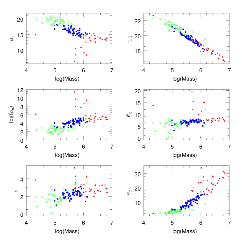
Figure 2: Binary diagrams of log(mass) vs $\mu_{0}$, $T_{1}$, log($\rho_{0}$), $W_{0}$, c, $\sigma_{p,0}$ for three groups. Blue solid squares are for G1, red solid triangles are for G2 and green empty circles are for G3.

It may be instructive to compare the structural properties of the GCs in NGC 5128 and in our own Galaxy. Fig.2 shows that mass is correlated with the other structural parameters c, $\mu_{0}$, $\rho_{0}$, $\sigma_{p,0}$, like in the Galaxy (Djorgovski & Meylan, 1994). On the other hand, unlike in our Galaxy, ellipticity (e), c, $\mu_{0}$ and $\rho_{0}$ are not correlated with $R_{gc}$.

The parameter $r_{h}$ is predicted to remain constant during the dynamical evolution of GCs, it is thus interesting to compare its value in our sample with that in other samples. We have compared the values of $r_{h}$ (King model) with the $r_{h}$ measured in a large sample of early-type galaxies by Jórdan et al. (2005). Note that these authors estimated $r_{h}$ using a King rather than Wilson model. Determining the peak of the distribution of $log(r_{h})$ for our whole sample with a nonparametric fit and Epanechnikov filter (Epanechnikov 1969), and assuming that this peak should fall at $r_{h}=2.85\pm 0.3$ pc, we find a distance to NGC5128 of $3.58\pm 0.3$ Mpc. The distance adopted in section 2 is within the error bars of this new distance estimate for NGC5128. The individual groups are too small to show any clear peak in the distribution of $r_{h}$.

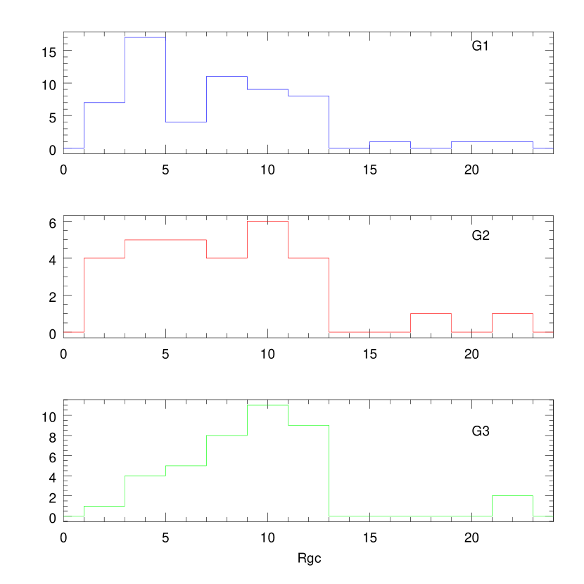
Figure 3: Histograms of $R_{gc}$ (galactocentric distance) for three groups. Colors are the same as in Fig2.

G3 is different from the two other groups in that it is mainly distributed in the outer regions of the galaxy (large $R_{gc}$, see Fig.3). Because most GCs of G3 are of low mass and thus of faint luminosity, no spectroscopy is available for them, and thus no age, radial velocity or spectroscopically determined metal abundance ([Z/H]). A possible consequence of this is that G3 might be polluted by foreground stars, although McLaughlin et al. (2008) only mention two possible such cases (C145, C152), by objects resembling intermediate-age Galactic open clusters (van den Bergh,2007), or by background galaxies.

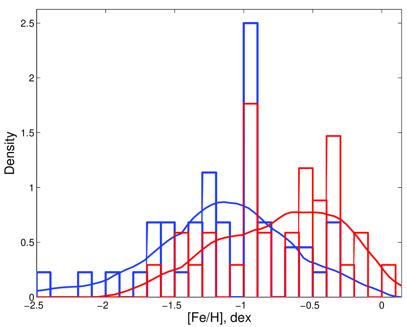
Figure 4: Probability density functions of [Fe/H] for the groups G1 and G2. Colors are the same as in Fig2.

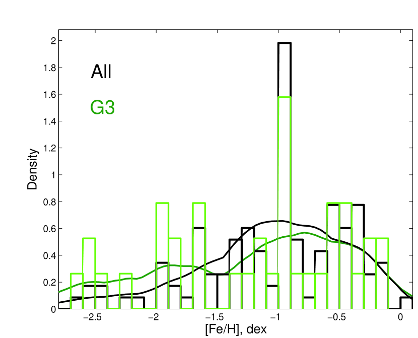
Figure 5: Probability density functions of [Fe/H] for the group G3 and the whole sample. Green is for G3 and black is for the entire sample.

The three groups have very different distributions of photometric metallicity [Fe/H], as shown by their probability density functions (PDF) in Figs. 4 and 5. The lines indicate non-parametric density estimates using an Epanechnikov kernel (Epanechnikov 1969). The bin width (0.2 dex for all groups) was chosen using the whole sample and the Freedman-Diaconis rule based on the sample size and the spread of the data (for a definition, see $"Freedman-Diaconis-rule"$ in wikipedia. For an explanation of the histogram as a density, see Freedman and Diaconis (1981)). A peak in the metallicity distribution at $[Fe/H]\sim-1$ is seen in all three groups. The PDF of G3 is clearly bimodal with a subgroup at very low metallicity, while the metallicity range of the two other groups is more limited and more in line with that of GCs in other galaxies, including our own. For example, our Galaxy has a distribution of [Fe/H] which peaks at -1.6 and -0.6 and the lowest value is -2.29 (Harris 2001). For M31, M 81 and NGC 4472, the numbers are respectively : -1.4, -0.6 and -2.18 (Barmby et al. 2000) -1.45, -0.53 and -2.0 (Ma et al. 2005) -1.3, -0.1 and -2.0 (Geisler et al. 1996).

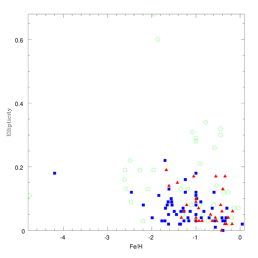
Figure 6: Binary plot of ellipticity vs [Fe/H] for the three groups. Colors and symbols are the same as in Fig.2.

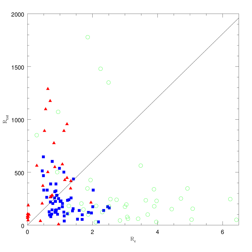
Figure 7: Color-color [Binary plot of tidal radii ($R_{tid}$) vs core radii ($R_{c}$) for the three groups. Colors and symbols are the same as in Fig2.

While metallicity and colors measure the state of evolution of the stellar populations, the structural parameters mainly give indications on the dynamical evolution of the GCs, and the three groups are markedly different in this respect as well. GCs are predicted to become rounder as they lose stars and angular momentum in the course of their evolution. In G1 the roundest GCs are also the most metal-rich, whereas no such correlation is present in G2 or G3, as shown on Fig.6. In G2, the roundest GCs are also the least massive. During the dynamical evolution of GCs, their $R_{c}$ shrinks and their $R_{tid}$ increases. Core collapse occurs when the ratio $log(R_{tid}/R_{c})>$ 2.5. As shown on Fig.7, this is the case for most GCs of G2 which are thus at an advanced stage of dynamical evolution, for a minority of GCs in G1, and for hardly any in G3.

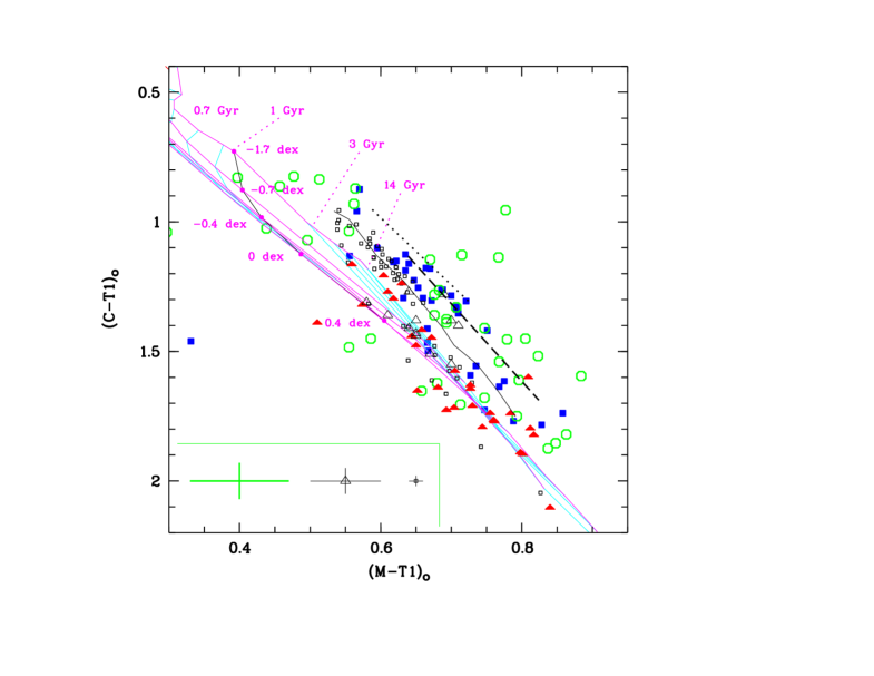
Figure 8: (M - $T_{1}$) vs (C - $T_{1}$)] plot in Washington photometry for the three groups of GCs of NGC 5128 (blue squares for G1, red triangles for G2 and green open circles for G3), LSB dwarf galaxies (open triangles), Galactic globular clusters (small open squares), SSP track of varying metallicity for an age of 15Gyr from Cellone & Forte (1996) (solid line), tracks for E galaxies (short-dashed line) and Sa galaxies (dotted line) from Buzzoni (2005). GALEV model grids (ages: from 140 Myr to 14 Gyr; metallicities: z=0.0004, 0.004, 0.008, 0.02, and 0.04) are over plotted (Anders & Fritze - v. Alvensleben, 2003). Seven GCs fall outside the plotted range, which has been reduced for clarity. The error bars are, from left to right, $\sigma(C-T_{1})=\pm 0.017and\sigma(M-T_{1})=\pm 0.009$ for Harris & Canterna (1977), $\pm 0.07$ in both colors for Harris et al.(2004), and $\pm 0.05$ in both colors for Cellone et al. (1994).

A color-color diagram is another way of examining the properties of the stellar populations of the GCs. This is done in Fig.8, which shows $(C-T_{1})_{o}$ vs $(M-T_{1})_{o}$ in the Washington photometric system for our sample, using data from Harris et al. (2004). For comparison, we also plotted on Fig.8 data for Galactic GCs (open squares, from Harris & Canterna 1977) and for low surface-brightness (LSB) dwarf galaxies (open triangles) from Cellone et al. (1994).

In order to interpret this Figure, we also plotted several model stellar populations : the thin black solid line is an SSP track of varying metallicity at 15Gyr from Cellone & Forte (1996). The thick short-dashed and dotted lines are tracks of varying age for ellipticals and Sa galaxies from Buzzoni (2005). The colored grid of models (metallicities z=0.0004, 0.004, 0.008, 0.02, and 0.04) are GALEV SSP models from Anders & Fritze - v. Alvensleben, (2003); they clearly show the extent of the age-metallicity degeneracy in this diagram. The three sets of models are based on different assumptions, and their differences are indicative of the uncertainties involved. The reddening line is roughly parallel to the tracks.

Before discussing Fig.8, we recall some relevant characteristics of the Washington photometric system. The C band includes the U-band and half of the B-band of the Johnson-Cousins photometric system (e.g. Lejeune 1996), and is thus sensitive to the presence of different features in the blue part of the color-magnitude diagram, such as extreme horizontal branch stars and abnormally wide main sequences, including branches of different colors. Such features are characteristics of the most massive Galactic GCs, probable cores of disrupted dwarf spheroidal satellites (Recio-Blanco et al. 2006). $C-T_{1}$ is almost twice as sensitive to age as to metallicity, and roughly three times more sensitive to both age and metallicity than $M-T_{1}$ (Cellone & Forte, 1996). One thus expects younger objects to have bluer $C-T_{1}$. The M and $T_{1}$ bands are equivalent to the Johnson-Cousins V and R bands, respectively. The M-band is centered on  500 nm, and includes the OIII 5007, OIII 4959, and H$\beta$ lines. The $T_{1}$ band is centered on the H$\alpha$ line, and on the [NII] 6548 and 6584 lines which are strong and in emission in planetary nebulae (PNe). The increase of $C-T_{1}$ may also be caused by the presence of PNe (and thus of Balmer emission lines). PNe are rare in GCs, as they are created during the final stages of the life of stars whose birth masses were between 1 and 8 M$\sun$; however, one can statistically expect a larger number of massive stars and thus of PNe in more massive GCs. There are only 4 known PNe in Galactic GCs (Jacoby et al. 1997) and there is one confirmed PN in the GCs of NGC 5128 (Minniti & Rejkuba 2002) and a few candidates (Rejkuba, Minniti & Walsh 2003). On the other hand, younger GCs have more PNe because of the higher range of progenitor masses (see also Larsen & Richtler 2006). (The authors thank the referee for the above discussion on planetary nebulae.)

Summarizing, metallicity increases the $C-T_{1}$ and $M-T_{1}$ colors in such a way that objects move along the reddening line on the color-color diagram, which is parallel to the SSP tracks of varying metallicity. Systematically redder $C-T_{1}$ at a given metallicity indicate older ages, redder horizontal branches, or the influence of emission-line objects on the integrated colors. This is why cores of disrupted dwarf galaxies, containing multiple stellar populations, may have bluer $(M-T_{1})$ and redder $C-T_{1}$ colors.

The GCs of G1 and G3 seem to be located roughly in the same region of the color-color diagram, but the scatter in G3 is large, presumably because the photometric uncertainties on these fainter objects are larger, and precludes any definite interpretation.

The GCs of G2 and a subset of LSB dwarf galaxies stand out in Fig.8 : most of them lie on a track of younger age and/or of higher metallicity than the GCs of G1 and the Galactic GCs. Cellone & Forte (1996) interpret the ”deviating branch” of LSB dwarf galaxies as caused by a mixture of stellar populations, including younger components. We adopt this interpretation for G2 and argue that the GCs of this group, which are the most massive GCs, have several generations of stars.

This property is shared by a growing number of massive GCs in our own Galaxy (Piotto, 2009 and references therein). However, these galactic GCs are metal-poor, while G2 is composed mostly of metal-rich GCs. Furthermore, galactic GCs appear to be intermediate between G2 and G1 in Fig 8; their average mass is 5.2 $\pm$ 0.6 in log(M/M_⊙), using the mass estimates of McLaughlin & Van Der Marel (2005), thus closer to G1 than to G2. In other words, the GCs in G2 bear little resemblance to the galactic GCs, and their large mass presumably allowed for multiple generations of stars more like what occurs in galaxies, thanks to their large potential well which retained the metals lost to the stars.

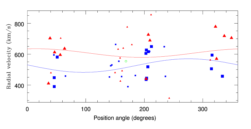
Figure 9: Radial velocity plotted against position angle (measured from North eastward) for the three groups (blue squares for G1, red triangles for G2, green open squares for G3). larger symbols denote radii larger than 8.0 arcmin. The mean rotation curves for the two first groups are shown as solid blue and red lines. The GCs of G2 have on average larger radial velocities than those of G1, their mean rotation curve is thus above that of G1.

The kinematic properties of the different groups may provide clues to their origin. G1 rotates in the same way as the majority of GCs and PNe of the galaxy (Woodley et al. 2007 and references therein), but has a lower mean velocity dispersion (102.1 km/s instead of $\simeq$ 110 km/s). G2 shows no significant mean rotation and a higher velocity dispersion than G1, comparable to that found by Woodley et al. (2007) for the GCs in the outer regions of the galaxy. The mean radial velocities of G1 and G2 are significantly different: that of G1 is close to the mean recession velocity of the galaxy, whereas that of G2 is much larger. This can be seen in Fig.9, which shows the radial velocity of the GCs against their position angle (measured from north eastward). This figure also shows that the rotation of G1 is marginal. Only one GC of G3 has a measured radial velocity. The gaps in position angle are due to the fact that the structural parameters were measured on several images which do not cover the galaxy uniformly.

5.4 Distinct origins of the three groups of globular clusters

We now proceed to interpret the distinctive properties of the three groups in view of explaining their possibly different origins; this must be done in the framework of the evolutionary history of the galaxy itself. We further have to assume that the structural characteristics of the GCs, on which this whole study is based, are indeed appropriate for discriminating between different histories of formation of GCs. While $r_{h}$ remains constant, all the other structural parameters change during the evolution. Furthermore, numerical simulations have shown that mass segregation and loss of low-mass stars have an effect on both the photometric and structural properties of GCs (e.g. Lamers et al. 2006). The distinct properties of the groups described in the preceding section do confort our working hypothesis, especially the fact that G2 is deviant in the color-color plot shown on Fig. 8.

NGC 5128 is an elliptical galaxy with a rotating dust lane (Graham, 1979) and a system of shells (Malin et al. 1983), both of which are characteristics of a past merger event, but not necessarily a unique one. Estimates for the age of the merger(s) range from 200 Myr to several Gyr (see Israel, 1998 for a review). The gaseous component associated with the dust lane is in rapid rotation about the major axis of the galaxy, in the same sense as G1, with a maximum rotation of 200 km/s for the ionized gas (Bland et al. 1987) and 265 km/s for the HI gas (van Gorkom et al. 1990). The gaseous disk is warped, and the gas is still unstable in the outer regions, two indications that the merger is recent. The stellar component of the galaxy rotates around the minor axis, with a maximum velocity of about 40 km/s (Wilkinson et al. 1986).

Considering first G2, it has no net rotation, is composed of old, massive, metal-rich and dynamically evolved GCs, and, because of its high mean radial velocity, might be associated with a high-velocity component of molecular gas (Israel 1998 and references therein). We propose that this group formed during the very first merger that gave rise to the elliptical galaxy. It is interesting to note that the metallicity distribution and age of G2 are very close to those of the outer halo stars of NGC 5128, for which Rejkuba et al. (2005) derived a mean metallicity of -0.64 and a mean age of 8 Gyr. It is thus tempting to assume that the GCs of G2 and the outer halo stars have the same origin.

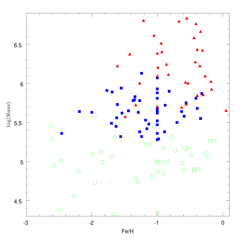
Figure 10: Mass-metallicity relation for the three groups (blue squares for G1, red triangles for G2, green open squares for G3).

The GCs of G2 are on average 9.4 Gyr old (see Table 4); however, considering that these are mostly massive GCs, this age might be influenced by the unwanted presence in the spectra of horizontal-branch stars, and in fact much older. Consequently, the merger may be even older than 9.4 Gyr, and at any rate much older than the one(s) that gave rise to the shells and dust lane. Mergers do produce a large number of super star clusters; for example, a thousand such clusters have been detected in NGC 4038/4039 (Mengel et al. 2005), a minority of which could later become massive GCs (Whitmore et al. 2007). Super star clusters in that and other recent merger remnants, NGC 7252 (Schweizer & Seitzer 1998), NGC 1275 (Zepf et al. 1995), are generally of solar metallicity. The metallicity of G2 is lower than solar, because the merger occurred at least 9.4 Gyr ago. Since G2 is composed of the most massive GCs of the sample, their high mass may be the cause of the multiple star formation episodes, more massive GCs being able to retain their metals for future generations of stars. A hint of a mass-metallicity relation can indeed be seen in Fig.10, if one ignores the low-mass GCs (those of G3), in the sense that there are no massive and metal-poor GCs in NGC 5128.

G3, on the contrary, is composed of low-mass, dynamically young GCs, and populates preferentially the external regions of the galaxy. This suggests that the GCs of this group were formed in satellite dwarf galaxies which were later progressively accreted into the halo of the galaxy and subsequently disrupted. It is likely that most accretion events occurred recently, since their probability increases with the mass of the attracting galaxy. The metallicity range of the metal-poor component of G3 points to progenitor galaxies of luminosities in the range $10^{8}-10^{9}L_{\odot}$, assuming that they have the same metallicity and a standard luminosity-metallicity relation (e.g. Lamareille et al 2009). The accretion and disruption of such low-mass galaxies could also explain a tidal stream of young stars discovered in the halo of NGC 5128 (Peng et al. 2002). Such accretion events may substantially increase the number of GCs in NGC 5128, because the number of GCs per unit galaxy mass ($S_{N}$) can be very high in the low-mass galaxies of the Centaurus group (e.g. $S_{N}$ = 100 for KK221, Puzia & Sharina, 2008). The metal-rich component of G3 might have originated in the accretion of slightly larger galaxies, like the LMC (see below), or, alternatively, be the low-mass end of G1 and/or G2.

The GCs of G1 have properties which are intermediate between those of G2 and G3, in mass and dynamical evolution. They are also marginally younger than those of G2. Furthermore, these GCs rotate in the same sense as the gaseous component, but much more slowly so. They might thus have originated in a galaxy that merged with NGC 5128, giving rise to the dust lane and maybe also the shells, and that is still in the process of settling dynamically in the merger remnant. Dynamical friction might be the cause of the slower velocity of rotation of the GCs of G1 compared to the gaseous component.

The peak at [Fe/H] = - 1 in all three groups may be an indication of a significant contribution of $10^{9}$ to $10^{10}M_{\odot}$ haloes during the hierarchical galaxy formation, assuming that these haloes produced GCs with roughly the same metallicity and that they follow the mass-metallicity relation at z $\simeq$ 1 (Lamareille et al. 2009). For comparison, we mention that the metallicity distribution of M87, another giant elliptical galaxy with an active nucleus, also peaks around - 1 (Cohen et al.1998), but, unlike NGC 5128, does not have a very low metallicity tail. There are in fact other analogies between the metallicity distributions of the three groups and those of GCs in nearby galaxies : for example between the GCs of M 31 (Barmby et al. 2000) and G1, or the GCs of the LMC (Beasley et al. 2002) and the metal-rich subgroup of G3. However, these comparisons can only give order of magnitude estimates, since the LMC may have been metal-enriched by interactions with our Galaxy, and M 31 might have a very different evolutionary history from the progenitor galaxy of G1, which merged at least 200 Myrs ago with NGC 5128.

In summary, the above scenario rests mainly on the assumption of accretion events which shaped the evolution of NGC 5128 and its GCs. The latter have several possible origins : the GCs of G2 were produced in a major merger, while the GCs of the two other groups were pre-existing in smaller galaxies that were subsequently accreted and disrupted. This favors the categories ii) and v) listed in the introduction for the formation of the galaxy itself, namely a major merger and several accretions and in-situ merging. The proposed scenario remains highly speculative, in the absence of spectroscopically determined ages and metallicities for most GCs in the galaxy.

6 Acknowledgements

TC and AKC are thankful to IUCAA for assistance through Associateship Programme. MES acknowledges of a partial support of a Russian Foundation Basic Research grant 08-02-00627. The authors are extremely grateful to Ethan T. Vishniac, Editor in Chief and Richard de Grijs (Scientific Editor) for their active cooperation and support. The authors are also very thankful to the referee for valuable suggestions and technical guidance in improving the quality of the work.

Appendix A PCA based on Multivariate MM-estimator with Fast and Robust Bootstrap

This method was developed by Salibián-Barrera et al.(2006). This Principal Component Analysis (PCA) is new in the sense that it is based on multivariate MM-estimator of shape instead of sample covariances. MM-estimator gives a robust estimate having the properties of maximum likelihood estimator. A robust estimate is not affected by outliers or small deviations from the model assumptions. The definitions of MM-estimators of Multivariate location and shape are given in the above mentioned paper. The-MM estimators were computed by applying the fast bootstrap procedure of Salibián-Barrera & Zamar (2002). If there are $p$ parameters in the data set and we denote the estimated variances of $p$ principal components by $\widehat{\lambda_{1}}>\widehat{\lambda_{2}}>...>\widehat{\lambda_{p}}$, then to find the optimum number of principal components the following proportion has been used (Salibián-Barrera et al. 2006) :

$$\begin{array}[]{ccc}\widehat{p}_{k}=\frac{\sum\limits_{j=1}^{k}\widehat{\lambda}_{j}}{\sum\limits_{j=1}^{p}\widehat{\lambda}_{j}},&for&k=1,...,p-1.\end{array}$$ (A1)

One should consider that value of k as optimum for which the value of 100$\widehat{p}_{k}$ exceeds some cut off value. In our case, this cut off value has been chosen as 90%. One can also test the hypothesis whether the actual proportion ${p}_{k}$ exceeds the cut off value 0.90% on the basis of an one sided confidence interval for ${p}_{k}$ based on the fast bootstrap.

Appendix B K-Means and mixture model methods of cluster analysis

The target of the mixture model method developed by Qui & Tamhane (2007) is to divide $n$ observations into $K(<n)$ clusters so that the within cluster variations are very small and any type of dissimilarity must occur between clusters. In this work Qui & Tamhane (2007) have assumed K to be known. In our analysis, we have computed the value of K by K-means clustering (MacQueen 1967) and a statistical technique developed by Sugar & James (2003). By using this algorithm we have first determined the structures of subpopulations (clusters) for varying number of clusters taking K = 1, 2, 3, 4 etc. For each such cluster formation we have computed the values of a distance measure $d_{K}=(1/p)min_{x}E[(x_{K}-c_{K})^{{}^{\prime}}(x_{K}-c_{K})]$ which is defined as the distance of the $x_{K}$ vector (values of the parameters) from the center $c_{K}$ (which is estimated as mean value), p is the order of the $x_{K}$ vector. Then the algorithm for determining the optimum number of clusters is as follows (Sugar & James 2003). Let us denote by $d_{K}^{\bf{}^{\prime}}$ the estimate of $d_{K}$ at the $K^{th}$ point. Then $d_{K}^{\bf{}^{\prime}}$ is the minimum achievable distortion associated with fitting K centers to the data. A natural way of choosing the number of clusters is to plot $d_{K}^{\bf{}^{\prime}}$ versus K and look for the resulting distortion curve. This curve is always monotonic decreasing. Initially one would expect much smaller drops i.e. a levelling off for K greater than the true number of clusters because past this point adding more centers simply partitions within groups rather than between groups. According to Sugar & James (2003) for a large number of items the distortion curve when transformed to an appropriate negative power ($p/2$ in our case), will exhibit a sharp ”jump” (if we plot K versus transformed $d_{K}^{\bf{}^{\prime}}$). Then we have calculated the jumps in the transformed distortion as $J_{K}=(d_{K}^{\bf{}^{\prime}-(p/2)}-d_{K-1}^{\bf{}^{\prime}-(p/2)}$). The optimum number of clusters is the value of K at which the distortion curve levels off as well as its value associated with the largest jump.
In this Mixture Model method the data has been considered as a mixture of k Multivariate distributions with unknown mixing proportions. The author have used EM algorithm to estimate the parameters of the Multivariate distributions considered in the model as well as the unknown mixing proportions. The method of maximization of the likelihood function (which is a part of the EM Algorithm) has been derived by McLachlan & Krishnan (1997).

Appendix C The Levenberg-Marquardt algorithm

In the present paper we have determined the rotation amplitudes ($\Omega$R) and the position angles of the axes of rotation (East of North) of different groups of GCs ($\psi_{0}$) obtained from the classification of GCs of NGC 5128. For this we have used the relation

$$v_{r}(\psi)=v_{sys}+\Omega Rsin(\psi-\psi_{0})$$ (C1)

(C$\widehat{o}$té et al. 2001; Richtler et al. 2004; Woodley et al. 2007). In the above equation, $v_{r}$ is the observed radial velocity of the GCs in the system, $v_{sys}$ is the galaxy’s systematic velocity, R is the projected radial distance of each GC from the center of the system assuming a distance of 3.8 Mpc to NGC 5128, and $\psi$ is the projected azimuthal angle of the GC measured in degrees east of north. The systematic velocity of NGC 5128 is held constant at $v_{sys}$ = 541 km$s^{-1}$ (Hui et al. 1995) for all kinematic calculations. The rotation axes of the different groups of GCs, $\psi_{0}$ and the product $\Omega$R, the rotation amplitudes are the values obtained from the numerical solution. We have used the Levenberg-Marquardt non-linear fitting Method (Levenberg 1944, Marquardt 1963) to solve the above equation.

The projected velocity dispersion is calculated using

$$\sigma_{v}^{2}=\sum_{i=1}^{N}\frac{(v_{fi}-v_{sys})^{2}}{N}$$ (C2)

(Woodley et al. 2007), where N is the number of clusters in each group of GCs, found as a result of the CA, $v_{fi}$ is the GC’s radial velocity after subtraction of rotational component determined with equation (C1) and $\sigma_{v}$ is the projected velocity dispersion.

Table 1: List of parameters of the globular clusters of NGC 5128 used in PCA and CA

Name	Group	c	$<\mu_{v}>_{h}$	$\mu_{0}$	$W_{0}$	log$R_{c}$	log$R_{tid}$	log$r_{h}$	log$M_{tot}$	$\rho_{0}$	$\sigma_{p,0}$	$t_{rh}$
			(mag $arcsec^{-2}$)	(mag $arcsec^{-2}$)		(pc)	(pc)	(pc)	($M_{\bigodot}$)	($M_{\bigodot}pc^{-3}$)	(km/sec)	($10^{9}$ years)
AAT111563	1	1.89	18.15	16.76	6.2	0.09	2.03	0.49	5.36	5129	6.90	0.91
AAT113992	1	2.46	19.10	16.97	7.1	0.15	2.64	0.75	5.68	5012	7.85	3.16
AAT115339	1	2.00	17.33	15.78	6.4	-0.03	2.01	0.40	5.53	16596	9.38	0.78
AAT119508	1	1.71	19.03	17.70	5.8	0.37	2.14	0.71	5.58	1380	6.84	2.51
AAT120336	1	2.24	18.50	16.66	6.8	0.13	2.41	0.64	5.64	6166	8.28	2.09
AAT120976	1	2.00	18.08	16.53	6.4	0.05	2.09	0.48	5.38	6761	7.21	0.91
C104	1	2.24	17.00	15.21	6.8	-0.12	2.16	0.39	5.62	33113	10.74	0.85
C115	1	1.71	18.35	17.09	5.8	0.29	2.06	0.64	5.56	2239	7.29	1.86
C123	1	2.17	18.38	16.64	6.7	-0.01	2.20	0.48	5.29	7586	6.62	0.83
C130	1	2.46	18.23	16.17	7.1	-0.04	2.45	0.56	5.45	11220	7.55	1.26
C133	1	2.11	17.08	15.40	6.6	-0.06	2.10	0.41	5.68	25704	11.09	0.95
C138	1	2.46	18.38	16.27	7.1	-0.05	2.45	0.55	5.42	10965	7.34	1.20
C140	1	1.89	18.48	17.02	6.2	0.20	2.14	0.60	5.48	3090	6.97	1.51
C146	1	2.31	18.38	16.45	6.9	0.01	2.36	0.55	5.50	9333	7.85	1.32
C147	1	1.75	18.98	17.65	5.9	0.27	2.08	0.63	5.32	1445	5.58	1.41
C149	1	2.17	17.48	15.78	6.7	-0.06	2.15	0.42	5.49	16982	8.83	0.83
C150	1	2.11	17.25	15.57	6.6	-0.13	2.02	0.34	5.47	26303	9.46	0.62
C154	1	2.24	18.25	16.45	6.8	0.11	2.38	0.62	5.62	6918	8.26	1.86
C157	1	2.54	17.58	15.36	7.2	-0.06	2.51	0.58	5.81	26915	11.30	1.90
C159	1	2.11	17.23	15.51	6.6	-0.17	1.98	0.30	5.55	40738	10.79	0.59
C160	1	1.84	18.00	16.58	6.1	0.05	1.94	0.44	5.36	6761	7.33	0.76
C164	1	1.46	17.05	15.95	5.1	0.05	1.59	0.33	5.52	12023	9.84	0.62
C167	1	2.38	18.53	16.54	7.0	-0.06	2.35	0.50	5.28	9333	6.50	0.89
F2GC14	1	2.70	19.33	16.84	7.4	-0.01	2.73	0.70	5.38	6457	6.15	1.95
F2GC31	1	2.31	18.53	16.64	6.9	0.004	2.35	0.54	5.32	6607	6.41	1.07
PFF034	1	2.24	18.05	16.26	6.8	0.09	2.37	0.60	5.63	7943	8.55	1.78
PFF041	1	2.54	17.13	14.94	7.2	-0.14	2.43	0.49	5.78	44668	11.97	1.38
PFF052	1	2.70	17.80	15.34	7.4	-0.15	2.59	0.56	5.65	30903	9.86	1.58
PFF059	1	2.62	18.63	16.24	7.3	0.05	2.70	0.72	5.81	12303	9.68	3.16
PFF063	1	2.79	17.28	14.70	7.5	-0.30	2.52	0.46	5.64	83176	11.30	1.07
PFF066	1	2.38	17.83	15.83	7.0	-0.02	2.40	0.55	5.65	16218	9.48	1.51
PFF083	1	2.95	17.70	14.69	7.7	-0.31	2.67	0.54	5.72	93325	11.72	1.58
R203	1	2.46	17.25	15.20	7.1	-0.15	2.34	0.45	5.63	36308	10.52	1.02
C113	1	2.62	16.98	14.67	7.3	-0.23	2.42	0.44	5.73	69183	12.16	1.10
C132	1	2.62	17.60	15.27	7.3	-0.06	2.59	0.61	5.83	27542	11.32	2.19
C137	1	2.87	17.83	15.01	7.6	-0.12	2.78	0.68	5.93	43652	12.39	3.09
PFF016	1	2.24	17.80	15.95	6.8	0.03	2.31	0.55	5.75	15488	10.45	1.66
PFF021	1	3.10	17.55	14.20	7.9	-0.31	2.81	0.65	5.91	128825	13.74	2.75
PFF023	1	2.17	16.88	15.14	6.7	-0.05	2.16	0.44	5.78	30903	12.19	1.15
PFF031	1	2.38	17.15	15.17	7.0	-0.07	2.35	0.50	5.79	30903	11.70	1.44
PFF035	1	2.00	17.83	16.22	6.4	0.15	2.19	0.58	5.87	10471	11.25	2.09
C043	1	1.94	16.58	15.09	6.3	0.14	2.13	0.56	6.13	20417	15.63	2.45
C135	1	2.38	16.80	14.82	7.0	-0.11	2.31	0.46	5.88	50119	13.68	1.38
C153	1	1.43	16.50	15.42	5.0	0.23	1.73	0.49	6.07	13183	15.31	1.82
G221	1	2.11	16.53	14.85	6.6	-0.07	2.08	0.40	5.90	47863	14.52	1.15
G293	1	2.00	15.78	14.27	6.4	-0.14	1.90	0.29	5.89	81283	16.14	0.76
PFF011	1	2.17	16.83	15.12	6.7	0.03	2.24	0.521	5.94	25119	13.30	1.78
AAT118198	2	3.32	16.53	10.81	9.8	-1.33	2.00	0.32	5.92	6.30957$\times 10^{7}$	23.50	0.91
C006	2	2.46	16.00	13.88	7.1	0.13	2.62	0.72	6.83	8.31764$\times 10^{4}$	30.34	8.91
C018	2	2.54	16.13	13.91	7.2	0.06	2.63	0.69	6.61	7.76247$\times 10^{4}$	24.95	6.31
C030	2	2.95	16.23	13.21	7.7	-0.09	2.89	0.76	6.79	2.39883$\times 10^{5}$	31.19	9.77
C032	2	3.27	16.78	12.51	8.3	-0.54	2.75	0.64	6.42	1.58489$\times 10^{6}$	28.12	4.47
C037	2	2.62	15.33	12.97	7.3	-0.34	2.31	0.33	6.24	4.89779$\times 10^{5}$	24.94	1.23
C142	2	2.54	15.85	13.63	7.2	-0.12	2.45	0.51	6.38	1.54882$\times 10^{5}$	23.33	2.69
C145	2	0.01	14.45	13.80	0.1	-0.02	0.87	0.06	6.00	9.54993$\times 10^{4}$	23.77	0.39
C152	2	1.94	14.08	12.57	6.3	-0.40	1.59	0.01	6.09	7.76247$\times 10^{5}$	27.60	0.36
F2GC69	2	5.23	16.60	6.32	19.5	-3.31	1.92	0.28	5.69	2.29087$\times 10^{11}$	18.32	0.63
G284	2	4.26	16.13	8.37	15.3	-2.42	1.83	0.20	5.73	4.78630$\times 10^{9}$	20.09	0.49
K131	2	3.40	15.28	9.15	11.1	-1.75	1.66	0.12	6.02	6.02560$\times 10^{8}$	33.96	0.50
PFF079	2	3.51	16.70	10.43	11.9	-1.61	1.90	0.38	5.72	8.51138$\times 10^{7}$	17.38	0.89
R223	2	4.20	15.98	8.35	15.1	-2.19	2.02	0.39	6.11	2.51189$\times 10^{9}$	25.00	1.38
C117	2	2.54	17.80	15.53	7.2	-0.08	2.50	0.56	5.85	3.31131$\times 10^{4}$	12.02	1.90
C168	2	2.87	19.25	16.43	7.6	0.05	2.95	0.85	5.70	7.94328$\times 10^{3}$	7.82	4.47
F1GC14	2	1.75	18.95	17.64	5.9	0.40	2.21	0.76	5.57	1.04713$\times 10^{3}$	6.41	2.82
PFF029	2	2.17	18.40	16.80	6.7	0.31	2.52	0.80	5.87	3.16228$\times 10^{3}$	8.95	4.36
C161	2	3.03	17.78	14.54	7.8	-0.34	2.71	0.56	5.84	1.47911$\times 10^{5}$	13.61	1.95
C003	2	3.30	17.80	13.37	8.4	-0.20	3.11	1.03	6.76	3.09030$\times 10^{5}$	27.10	23.44
C004	2	2.00	16.78	15.25	6.4	0.29	2.33	0.72	6.37	1.23027$\times 10^{4}$	16.98	5.37
C007	2	2.87	16.58	13.77	7.6	0.08	2.98	0.8	6.80	7.94328$\times 10^{4}$	26.85	14.79
C012	2	3.27	3.27	3.27	3.27	3.27	3.27	3.27	3.27	3.27000$\times 10^{0}$	3.27	3.27
C014	2	2.70	16.68	14.19	7.40	0.03	2.76	0.74	6.51	6.60693$\times 10^{4}$	21.58	6.76
C019	2	2.38	16.70	14.70	7.00	0.12	2.54	0.69	6.40	3.38844$\times 10^{4}$	19.01	5.13
C025	2	3.20	17.45	13.60	8.10	-0.28	2.95	0.79	6.43	3.01995$\times 10^{5}$	22.44	7.58
C029	2	3.20	17.65	13.80	8.10	-0.16	3.07	0.92	6.58	1.81970$\times 10^{5}$	23.28	13.49
C036	2	2.54	16.03	13.83	7.20	-0.13	2.44	0.50	6.22	1.20226$\times 10^{5}$	19.91	2.19
C139	2	2.87	16.85	14.00	7.60	-0.32	2.57	0.48	6.00	2.13796$\times 10^{5}$	17.18	1.66
C151	2	2.24	17.43	15.53	6.80	-0.18	2.10	0.34	5.65	5.12861$\times 10^{4}$	11.83	0.76
C165	2	2.79	17.25	14.57	7.50	-0.08	2.74	0.68	6.27	7.58578$\times 10^{4}$	18.11	4.36
G170	2	2.46	17.00	14.88	7.10	-0.08	2.41	0.52	6.01	5.24807$\times 10^{4}$	15.03	1.95
WHH09	2	2.54	17.63	15.35	7.20	0.08	2.65	0.72	6.22	2.63027$\times 10^{4}$	15.45	4.79
WHH16	2	2.54	16.83	14.55	7.20	-0.15	2.42	0.48	6.09	1.00000$\times 10^{5}$	17.38	1.82
WHH22	2	2.87	16.73	13.91	7.60	-0.20	2.70	0.60	6.20	1.44544$\times 10^{5}$	18.62	3.02
C126	3	3.86	21.80	14.93	13.7	-1.59	2.27	0.71	4.33	1258925	2.24	0.74
AAT117287	3	1.80	19.20	17.87	6.0	0.39	2.24	0.76	5.47	871	5.71	2.57
C111	3	3.03	21.33	18.18	7.8	-0.02	3.03	0.88	4.88	1820	3.12	2.24
C114	3	1.52	22.28	21.08	5.3	0.80	2.39	1.08	5.11	28	2.58	5.89
C118	3	2.70	20.65	18.12	7.4	-0.04	2.70	0.67	4.90	2630	3.66	1.15
C124	3	1.67	20.73	19.49	5.7	0.36	2.09	0.69	4.74	214	2.65	1.05
C125	3	1.89	19.95	18.48	6.2	0.32	2.26	0.72	5.17	646	4.24	1.74
C127	3	2.24	21.08	19.25	6.8	0.27	2.54	0.78	4.81	347	2.70	1.51
C131	3	1.89	19.30	17.89	6.2	0.30	2.24	0.70	5.31	1047	5.09	1.82
C136	3	1.49	18.95	17.85	5.2	0.19	1.75	0.47	4.99	1413	4.57	0.60
C143	3	0.99	18.93	18.12	3.1	0.34	1.48	0.50	5.06	759	4.82	0.71
C158	3	1.89	19.75	18.30	6.2	0.44	2.38	0.84	5.45	575	5.14	3.31
C163	3	1.17	19.55	18.65	4.0	0.49	1.78	0.69	5.22	347	4.59	1.58
C170	3	1.89	20.25	18.80	6.2	0.10	2.04	0.50	4.56	759	2.72	0.45
C172	3	1.71	19.23	17.97	5.8	0.23	1.99	0.57	5.09	1175	4.55	0.93
C174	3	2.11	19.83	18.12	6.6	0.10	2.26	0.57	4.98	1698	4.11	0.87
C176	3	2.05	20.10	18.56	6.5	0.22	2.31	0.67	4.95	724	3.52	1.15
C179	3	1.32	20.20	19.25	4.6	0.49	1.89	0.72	5.01	204	3.48	1.48
F2GC18	3	2.70	19.20	16.72	7.4	-0.22	2.52	0.49	4.99	11220	5.01	0.66
F2GC20	3	1.67	19.58	18.28	5.7	0.27	2.00	0.60	5.16	1047	4.76	1.15
F2GC28	3	1.05	19.90	19.04	3.4	0.45	1.64	0.62	5.00	288	3.87	1.05
C105	3	1.59	21.80	20.57	5.5	0.59	2.25	0.90	4.88	63	2.45	2.51
C112	3	0.01	20.53	19.86	0.1	0.60	1.48	0.68	4.85	95	3.12	1.12
C119	3	1.94	20.03	18.67	6.3	0.41	2.39	0.82	5.27	457	4.28	2.69
C120	3	0.16	21.68	20.97	0.2	0.81	1.70	0.89	4.89	24	2.54	2.40
C121	3	0.93	20.53	19.78	2.8	0.32	1.43	0.47	4.38	182	2.28	0.35
C122	3	1.89	21.53	20.08	6.2	0.24	2.17	0.63	4.34	178	1.81	0.59
C128	3	1.71	21.28	19.91	5.8	0.60	2.36	0.94	5.27	135	3.65	4.17
C129	3	1.71	20.60	19.28	5.8	0.48	2.24	0.82	5.14	234	3.62	2.34
C134	3	2.79	21.58	18.92	7.5	0.35	3.17	1.11	5.31	437	3.66	7.41
C141	3	1.40	21.08	20.06	4.9	0.71	2.19	0.96	5.12	56	3.01	3.72
C144	3	1.35	21.30	20.33	4.7	0.57	2.00	0.81	4.73	60	2.28	1.55
C148	3	1.67	20.50	19.31	5.7	0.67	2.40	1.00	5.45	129	4.21	5.89
C155	3	1.89	21.65	20.19	6.2	0.59	2.53	0.99	5.00	71	2.58	3.63
C162	3	2.17	21.05	19.38	6.7	0.54	2.75	1.03	5.29	162	3.48	5.62
C166	3	0.76	21.15	20.41	1.9	0.70	1.72	0.82	4.87	44	2.68	1.82
C171	3	1.46	20.73	19.62	5.1	0.65	2.18	0.92	5.22	102	3.53	3.55
C173	3	1.75	21.13	19.74	5.9	0.56	2.37	0.92	5.26	170	3.72	3.80
C175	3	2.95	22.38	19.37	7.7	0.27	3.25	1.12	4.99	331	2.62	5.75
C178	3	1.75	21.33	20.02	5.9	0.48	2.29	0.84	4.79	98	2.37	1.78
F1GC20	3	1.80	21.80	20.41	6.0	0.69	2.54	1.06	5.17	55	2.86	5.62
F1GC21	3	1.80	20.85	19.43	6.0	0.40	2.25	0.77	5.06	324	3.53	1.86
F1GC34	3	1.13	20.40	19.47	3.8	0.53	1.78	0.72	5.08	195	3.78	1.62
F2GC70	3	2.70	20.65	18.21	7.4	0.40	3.13	1.11	5.59	646	4.93	9.77
C116	3	2.31	21.45	19.51	6.9	0.29	2.63	0.83	4.90	355	2.87	2.00
C156	*	3.03	11.21	7.95	7.80	-1.49	1.56	-0.59	6.22	9	1.90	7.72
C169	*	3.27	22.29	18.13	8.30	0.31	3.60	1.49	5.71	2.93	0.67	10.61
F1GC15	*	3.48	21.52	15.22	11.70	-0.55	2.93	1.41	6.14	5.19	0.94	10.69

Note. — Values in column 1 and in columns 3 to 13 are from McLaughlin et al.(2008).Column 2 represents the group membership found as a result of CA.

Table 2: List of parameters as well as derived parameters of the globular clusters of NGC 5128.

Name	Group	$R_{gc}$	$T_{1}$	[Fe/H]	$(C-T_{1})_{0}$	$V_{r}$	[Z/H]	Age	$V_{rot}$	$\sigma_{v}$
		(kpc)	(mag)	(dex)	(mag)	(km/sec)	(dex)	(Gyr)	(km/sec)	(km/sec)
AAT111563	1	11.93	20.05	-2.46	0.87	649	$\cdots$	$\cdots$	43.96 for G1	102.08 for G1
AAT113992	1	4.26	19.82	-0.39	1.74	648	$\cdots$	$\cdots$
AAT115339	1	3.82	19.56	-1.18	1.33	618	$\cdots$	$\cdots$
AAT119508	1	4.12	19.86	-0.59	1.62	$\cdots$	$\cdots$	$\cdots$
AAT120336	1	7.16	19.67	-0.63	1.59	452	$\cdots$	$\cdots$
AAT120976	1	7.56	19.99	-1.27	1.29	595	$\cdots$	$\cdots$
C104	1	8.96	19.40	-1.54	1.19	448	$\cdots$	$\cdots$
C115	1	12.30	19.51	-1.62	1.16	$\cdots$	$\cdots$	$\cdots$
C123	1	10.46	20.24	-0.98	1.42	$\cdots$	$\cdots$	$\cdots$
C130	1	10.92	19.85	-1.63	1.15	$\cdots$	$\cdots$	$\cdots$
C133	1	3.37	19.30	-1.00	1.40	$\cdots$	$\cdots$	$\cdots$
C138	1	3.08	19.97	-1.16	1.34	$\cdots$	$\cdots$	$\cdots$
C140	1	3.25	19.83	-1.13	1.35	$\cdots$	$\cdots$	$\cdots$
C146	1	4.45	19.94	-0.70	1.56	$\cdots$	$\cdots$	$\cdots$
C147	1	2.98	20.06	-1.24	1.31	$\cdots$	$\cdots$	$\cdots$
C149	1	6.85	19.68	-1.70	1.13	389	$\cdots$	$\cdots$
C150	1	2.24	19.78	-1.00	1.40	$\cdots$	$\cdots$	$\cdots$
C154	1	2.97	19.58	-1.00	1.40	$\cdots$	$\cdots$	$\cdots$
C157	1	3.38	19.21	-1.00	1.40	$\cdots$	$\cdots$	$\cdots$
C159	1	4.44	19.93	-0.34	1.77	$\cdots$	$\cdots$	$\cdots$
C160	1	3.33	19.99	-1.00	1.40	$\cdots$	$\cdots$	$\cdots$
C164	1	3.79	19.60	-1.00	1.40	$\cdots$	$\cdots$	$\cdots$
C167	1	7.22	20.41	-1.00	1.40	$\cdots$	$\cdots$	$\cdots$
F2GC14	1	6.97	20.82	-0.89	1.46	$\cdots$	$\cdots$	$\cdots$
F2GC31	1	7.25	20.15	-1.56	1.18	$\cdots$	$\cdots$	$\cdots$
PFF034	1	12.62	19.38	-1.29	1.28	605	$\cdots$	$\cdots$
PFF041	1	4.00	19.01	-1.37	1.25	456	$\cdots$	$\cdots$
PFF052	1	4.58	19.42	-1.44	1.22	462	$\cdots$	$\cdots$
PFF059	1	4.00	19.48	-0.41	1.73	525	$\cdots$	$\cdots$
PFF063	1	8.17	19.45	-2.19	0.96	554	$\cdots$	$\cdots$
PFF066	1	6.79	19.44	-1.00	1.41	530	-0.81$\pm$0.18	12:
PFF083	1	7.61	19.44	-0.88	1.47	458	$\cdots$	$\cdots$
R203	1	8.32	19.38	-2.00	1.02	455	-1.02$\pm$0.12	6.1$\pm$1.1
C113	1	19.68	19.12	-1.61	1.16	$\cdots$	$\cdots$	$\cdots$
C132	1	9.64	18.90	-1.34	1.26	436	$\cdots$	$\cdots$	$\cdots$	$\cdots$
C137	1	2.67	19.04	-1.00	1.40	$\cdots$	$\cdots$	$\cdots$
PFF016	1	12.56	19.33	-0.56	1.64	505	-0.35$\pm$0.38	10.5:
PFF021	1	9.71	18.81	-1.77	1.10	594	$\cdots$	$\cdots$
PFF023	1	15.02	18.97	-1.27	1.29	457	-1.06$\pm$0.13	7.0$\pm$1.2
PFF031	1	12.35	18.95	-1.35	1.26	444	$\cdots$	$\cdots$
PFF035	1	11.66	19.13	-0.32	1.78	627	$\cdots$	$\cdots$
C043	1	10.47	18.07	-1.24	1.30	518	-1.21$\pm$0.04	12.0$\pm$2.2
C135	1	2.75	18.90	-1.00	1.40	$\cdots$	$\cdots$	$\cdots$
C153	1	2.93	18.23	-1.00	1.40	$\cdots$	$\cdots$	$\cdots$
G221	1	9.41	18.83	-0.82	1.50	390	$\cdots$	$\cdots$
G293	1	9.50	18.69	-1.69	1.13	581	-1.29$\pm$0.07	12.0$\pm$3.6
PFF011	1	22.51	18.55	-1.55	1.18	616	$\cdots$	$\cdots$
AAT118198	2	5.46	19.03	-0.17	1.89	575	$\cdots$	$\cdots$	27.94 for G2	121.58 for G2
C006	2	2.10	16.51	-0.55	1.64	$\cdots$	-0.51:	11.00:
C018	2	4.95	16.89	-1.05	1.39	480	-0.71$\pm$0.10	8.0$\pm$1.6
C030	2	10.87	16.68	-0.67	1.57	778	-0.27$\pm$0.05	6.6$\pm$1.4
C032	2	12.47	17.85	-0.31	1.79	718	-0.10$\pm$0.20	13:
C037	2	11.95	17.96	-0.86	1.47	612	-0.53$\pm$0.19	12.0$\pm$4.0
C142	2	1.85	17.64	-1.00	1.40	$\cdots$	$\cdots$	$\cdots$
C145	2	3.56	17.81	-1.27	1.29	$\cdots$	$\cdots$	$\cdots$
C152	2	2.75	17.82	-1.00	1.40	$\cdots$	$\cdots$	$\cdots$
F2GC69	2	10.51	19.30	-0.63	1.60	$\cdots$	$\cdots$	$\cdots$
G284	2	5.93	19.41	-0.56	1.64	479	$\cdots$	$\cdots$
K131	2	3.84	18.74	-0.18	1.89	639	$\cdots$	$\cdots$
PFF079	2	10.72	19.14	-1.33	1.27	410	$\cdots$	$\cdots$
R223	2	6.60	18.19	-0.83	1.49	776	$\cdots$	$\cdots$
C117	2	9.73	19.26	-0.30	1.79	$\cdots$	$\cdots$	$\cdots$
C168	2	7.91	19.71	-1.00	1.40	$\cdots$	$\cdots$	$\cdots$
F1GC14	2	12.11	19.67	-1.49	1.20	$\cdots$	$\cdots$	$\cdots$
PFF029	2	8.87	19.10	-4.20	0.40	570	$\cdots$	$\cdots$
C161	2	7.28	19.26	-0.39	1.74	425	$\cdots$	$\cdots$
C003	2	8.10	17.08	-0.41	1.72	562	-0.13$\pm$0.05	5.8$\pm$1.2
C004	2	10.53	17.50	-1.42	1.23	689	-1.44$\pm$0.12	10:
C007	2	9.18	16.64	-1.21	1.32	595	-0.93$\pm$0.09	12.0$\pm$4.0
C012	2	11.26	17.36	-0.34	1.77	$\cdots$	$\cdots$	$\cdots$
C014	2	18.31	17.41	-0.94	1.44	705	-0.85$\pm$0.16	10.0$\pm$4.0
C019	2	7.59	17.55	-0.93	1.44	632	-0.91$\pm$0.14	12:
C025	2	8.49	17.96	-0.39	1.74	703	-0.21$\pm$0.07	8.0$\pm$2.6
C029	2	21.02	17.53	-0.44	1.71	726	-0.17$\pm$0.05	8.0$\pm$1.8
C036	2	12.95	17.94	-1.61	1.16	703	-1.07$\pm$0.12	12:
C139	2	2.77	18.86	-0.53	1.65	$\cdots$	$\cdots$	$\cdots$
C151	2	3.26	19.95	0.05	2.10	$\cdots$	$\cdots$	$\cdots$
C165	2	5.27	18.17	-0.42	1.71	$\cdots$	$\cdots$	$\cdots$
G170	2	8.86	18.73	-0.57	1.63	636	-0.26$\pm$0.18	12:
WHH09	2	4.35	18.30	-0.35	1.76	315	$\cdots$	$\cdots$
WHH16	2	3.19	18.60	-0.27	1.82	661	-0.20$\pm$0.04	8.0$\pm$0.02
WHH22	2	5.04	18.03	-0.99	1.41	$\cdots$	$\cdots$	$\cdots$
C126	3	10.45	22.66	-1.67	1.14	$\cdots$	$\cdots$	$\cdots$	$\cdots$	$\cdots$
AAT117287	3	3.53	20.45	-1.62	1.16	554	$\cdots$	$\cdots$
C111	3	21.69	21.36	-2.20	0.96	$\cdots$	$\cdots$	$\cdots$
C114	3	12.67	21.42	-0.27	1.82	$\cdots$	$\cdots$	$\cdots$
C118	3	10.38	20.67	-0.44	1.71	$\cdots$	$\cdots$	$\cdots$
C124	3	11.99	21.57	-1.30	1.28	$\cdots$	$\cdots$	$\cdots$
C125	3	12.34	20.66	-0.91	1.45	$\cdots$	$\cdots$	$\cdots$
C127	3	9.92	21.62	-1.08	1.38	$\cdots$	$\cdots$	$\cdots$
C131	3	11.85	20.20	-1.65	1.15	$\cdots$	$\cdots$	$\cdots$
C136	3	3.84	21.19	-1.84	1.08	$\cdots$	$\cdots$	$\cdots$
C143	3	2.45	20.52	-1.70	1.13	$\cdots$	$\cdots$	$\cdots$
C158	3	5.39	20.06	-1.05	1.39	$\cdots$	$\cdots$	$\cdots$
C163	3	4.05	20.43	-1.18	1.33	$\cdots$	$\cdots$	$\cdots$
C170	3	7.93	22.16	-2.27	0.93	$\cdots$	$\cdots$	$\cdots$
C172	3	10.83	20.91	-1.99	1.02	$\cdots$	$\cdots$	$\cdots$
C174	3	9.17	21.42	-0.63	1.60	$\cdots$	$\cdots$	$\cdots$
C176	3	8.41	21.30	-2.58	0.84	$\cdots$	$\cdots$	$\cdots$
C179	3	9.91	21.04	-2.47	0.87	$\cdots$	$\cdots$	$\cdots$
F2GC18	3	6.93	21.15	-1.00	1.40	$\cdots$	$\cdots$	$\cdots$
F2GC20	3	6.59	21.01	-0.53	1.65	$\cdots$	$\cdots$	$\cdots$
F2GC28	3	6.39	21.16	-0.84	1.48	$\cdots$	$\cdots$	$\cdots$
C105	3	9.73	21.76	-0.44	1.70	$\cdots$	$\cdots$	$\cdots$
C112	3	22.46	21.31	-0.91	1.45	$\cdots$	$\cdots$	$\cdots$
C119	3	8.45	20.67	-4.77	0.27	$\cdots$	$\cdots$	$\cdots$
C120	3	11.67	21.43	-0.60	1.61	$\cdots$	$\cdots$	$\cdots$
C121	3	9.91	22.45	-2.49	0.86	$\cdots$	$\cdots$	$\cdots$
C122	3	9.84	22.33	-1.00	1.40	$\cdots$	$\cdots$	$\cdots$
C128	3	9.74	20.95	-0.14	1.91	$\cdots$	$\cdots$	$\cdots$
C129	3	12.53	20.83	-0.73	1.54	$\cdots$	$\cdots$	$\cdots$
C134	3	3.29	20.71	-0.78	1.52	$\cdots$	$\cdots$	$\cdots$
C141	3	2.68	20.94	-1.86	1.07	$\cdots$	$\cdots$	$\cdots$
C144	3	3.87	21.96	-1.95	1.04	$\cdots$	$\cdots$	$\cdots$
C148	3	5.17	20.21	-2.62	0.82	$\cdots$	$\cdots$	$\cdots$
C155	3	7.85	21.36	-1.00	1.41	$\cdots$	$\cdots$	$\cdots$
C162	3	5.04	20.91	-2.60	0.83	$\cdots$	$\cdots$	$\cdots$
C166	3	4.97	20.72	-1.00	1.40	$\cdots$	$\cdots$	$\cdots$
C171	3	8.64	20.67	-1.11	1.36	$\cdots$	$\cdots$	$\cdots$
C173	3	9.35	21.06	-0.19	1.88	$\cdots$	$\cdots$	$\cdots$
C175	3	7.35	21.84	-0.91	1.45	$\cdots$	$\cdots$	$\cdots$
C178	3	8.78	21.53	-1.34	1.26	$\cdots$	$\cdots$	$\cdots$
F1GC20	3	9.95	21.22	-0.58	1.62	$\cdots$	$\cdots$	$\cdots$
F1GC21	3	11.01	21.36	-0.22	1.85	$\cdots$	$\cdots$	$\cdots$
F1GC34	3	12.16	20.96	-0.48	1.68	$\cdots$	$\cdots$	$\cdots$
F2GC70	3	9.36	20.04	-1.96	1.04	$\cdots$	$\cdots$	$\cdots$
C116	3	11.72	21.84	-0.37	1.75	$\cdots$	$\cdots$	$\cdots$
C156	*	4.83	17.65	-0.18	1.89	$\cdots$	$\cdots$	$\cdots$
C169	*	7.74	20.39	-2.08	1.00	$\cdots$	$\cdots$	$\cdots$
F1GC15	*	12.11	19.53	-0.04	2.01	$\cdots$	$\cdots$	$\cdots$

Note. — Values in column 1 and in columns 3 to 6 are from McLaughlin et al .(2008), column 2 represents the group membership found by CA,values in column 7 are from Woodley et al. (2007), values in columns 8 to 11 have been derived in the present work.

Note. — ’:’s are used for the errors of [Z/H]s and Ages when error of [Z/H] $>0.4$ dex and error of Age $>4$ Gyr

Table 3: Result of PCA analysis

Set	components	% of	no. of	eigen		significant
		variations	significant	vectors		parameters
			eigen
			vectors
			corresponding
			to variation
			$>$ 90%	(1)	(2)
S1([Fe/H],	1	67.54	2	(0.0164,	(-0.0233,	T1,
T1,c,$\mu_{0}$,	2*	91.95*		-0.1712,	-0.0121,	$\mu_{0}$,
W0,Rc,	3	97.95		0.0396,	-0.0006,	rh,
rh,$\sigma_{p,0}$,	4	98.90		-0.2641,	0.0185,	$\sigma_{p,0}$,
Rgc)	5	99.50		0.0638,	0.0012,	Rgc
	6	99.90		-0.0906,	0.0188,
	7	99.97		-0.1053,	0.0526,
	8	99.99		0.9348,	0.0587,
	9	100.00		-0.0446)	0.9962)
S2($\mu_{0}$,rh,	1	70.44	2	(-0.2960,	(0.0179,	$\mu_{0}$,
$\sigma_{p,0}$,Rgc)	2*	93.29*		-0.1281,	0.0945,	Rh,
	3	99.38		0.9430,	0.0933,	$\sigma_{p,0}$,
	4	100.00		-0.0714)	0.9909)	Rgc
S3($\mu_{0}$,rh,	1*	90.39*	1	(-0.2924,		$\mu_{0}$,
$\sigma_{p,0}$,c)	2	98.93		-0.1174,		Rh,
	3	99.89		0.947,		$\sigma_{p,0}$,
	4	100.00		0.100)		c
S4($\mu_{0}$,rh,	1	91.35*	1	(-0.3003,		$\mu_{0}$,
$\sigma_{p,0}$)	2	99.23		-0.1291,		Rh,
	3	100.00		0.9450)		$\sigma_{p,0}$
S5([Fe/H],	1	71.72	2	(-0.135,	(0.957,	[Fe/H],
c,Rc)	2*	91.6*		-0.488,	0.160,	c,
	3	100.00		0.861)	0.240)	Rc
S6($\mu_{0}$,rh,	1	88.99*	1	(-0.2821,		$\mu_{0}$,
$\sigma_{p,0}$,W0)	2*	98.15		-0.1130,		Rh,
	3	99.78		0.9486,		$\sigma_{p,0}$,
	4	100.00		0.100)		W0
S7($<\mu_{v}>_{h},r_{h},\sigma_{p,0}$)	1	91.78*	1	(-0.238,		$<\mu_{v}>_{h}$,
	2	99.57		-0.149,		$r_{h}$,
	3	100.00		0.9600)		$\sigma_{p,0}$
S8($<\mu_{v}>_{h},r_{h},\sigma_{p,0}$	1	88.51	2	(-0.216,	(0.333,	$<\mu_{v}>_{h}$,
$,W_{0}$)	2	98.39*		-0.110,	0.926,	$r_{h}$,
	3	99.62		-0.967,	0.178,	$\sigma_{p,0}$,
	4	100.00		0.079)	0.031)	$W_{0}$
S9($<\mu_{v}>_{h},r_{h},\sigma_{p,0},c$)	1	90.13*	1	(-0.222,		$<\mu_{v}>_{h}$,
	2	99.14		-0.120,		$r_{h}$,
	3	99.59		0.966,		$\sigma_{p,0}$,
	4	100.00		0.056)		c

Table 4: Mean values of the observed and derived parameters in three groups of GCs found by CA

	G1	G2	G3
No	47	35	45
Age (Gyr)	10.202$\pm 0.845$	9.447$\pm 0.814$	$\cdots$
$\left[Z/H\right]$ (dex)	-0.985$\pm 0.152$	-0.553$\pm 0.105$	$\cdots$
$\mu_{0}$ $(mag~{}arcsec^{-2})$	15.828$\pm 0.127$	13.414$\pm 0.412$	19.077$\pm 0.170$
log$R_{c}$ (pc)	-0.011$\pm$0.022	-0.429$\pm$0.142	0.363$\pm$0.055
log$R_{tid}$ (pc)	2.284$\pm$0.039	2.432$\pm$0.082	2.244$\pm$0.064
log$r_{h}$ (pc)	0.523$\pm$0.0162	0.571$\pm$0.043	0.786$\pm$0.027
log$M_{tot}$ $(M_{\odot})$	5.642$\pm$0.031	6.187$\pm$0.062	5.023$\pm$0.042
$\rho_{0}$ $(M_{\odot}pc^{-3})$	(2.605$\pm 0.039$)$\times$104	(6.773$\pm 6.54$)$\times$109	(2.870$\pm 2.79$)$\times$103
$\sigma_{p,0}$ (km/sec)	9.984$\pm$0.400	20.528$\pm 1.130$	3.533$\pm 0.144$
$t_{rh}$ ($10^{9}$ years)	1.502$\pm$0.099	4.762$\pm$0.088	2.538$\pm$0.309
Rgc (kpc)	7.532$\pm 0.660$	7.992$\pm 0.745$	8.938$\pm 0.613$
T1 (mag)	19.462$\pm 0.081$	18.218$\pm 0.159$	21.156$\pm 0.092$
$[Fe/H]$ (dex)	-1.172$\pm 0.068$	-0.816$\pm 0.122$	-1.317$\pm 0.134$
$(C-T_{1})_{0}$ (mag)	1.349$\pm$0.030	1.539$\pm$0.050	1.322$\pm$0.052
$c$	2.255$\pm$0.053	2.811$\pm$ 0.142	1.784$\pm$0.106
$W_{0}$	6.749$\pm$0.088	8.246$\pm$0.539	5.662$\pm$0.316
$<\mu_{v}>_{h}$ $(mag~{}arcsec^{-2})$	17.722$\pm$0.114	16.778$\pm$0.185	20.640$\pm$0.136
$V_{r}$ (km/sec)	520.5$\pm$16.5	608.6$\pm$26.3	$\cdots$
e (Ellipticity)	0.068$\pm$0.05	0.157$\pm$0.14	0.068$\pm$0.04
Vrot (km/sec)	43.96	27.94	$\cdots$
$\theta_{0}$ $(deg)$	185.83(major)	285.12(minor)	$\cdots$
$\sigma_{v}$ (km/sec)	102.082	121.578	$\cdots$
x	0.43	0.23	$\cdots$
$\Lambda$=0.3x	0.129	0.069	$\cdots$

References

- Anders & v. Alvensleben (2003) Anders P., & v. Alvensleben U.F., 2003, A&A 401,1063.
- Arimoto & Joshi (1987) Arimoto N., & Yoshii Y., 1987, A&A, 173, 23.
- Ashman & Sepf (1992) Ashman K.M., & Zepf S.E., 1992, ApJ, 384, 50.
- Barmby et al. (2000) Barmby P., Huchra J.P., Brodie J.P. et al., 2000, AJ 119, 727
- Beasley et al. (2008) Beasley M.A., Bridges T., Peng E. et al. 2008, MNRAS, 386, 1443.
- Bekki et al. (2002) Bekki K., Forbes D.A., Beasley M.A., & Couch W.J. 2002, MNRAS, 335,1176.
- Bland et al (1987) Bland J., Taylor K., & Atherton P.D. 1987, MNRAS 228, 595.
- Buzzoni (2005) Buzzoni A. 2005, MNRAS, 361,725.
- Carlberg (1984) Carlberg R.G. 1984, ApJ, 286,403.
- Cellone & Forte (1996) Cellone S.A., & Forte J.C. 1996, ApJ, 461, 176.
- Cellone et al. (1994) Cellone S.A., Forte J.C., & Geisler D. 1994, ApJS 93, 397.
- Cohen et al. (1998) Cohen J.G., Blakeslee J.P., & Ryzhov A. 1998, ApJ, 496, 808.
- Cté et al. (1998) Cté P., Marzke R.O., & West M.J. 1998, ApJ, 501, 554.
- Djorgovski (1995) Djorgovski S. 1995, ApJ, 438, L29.
- Djorgovski& Meylan (1994) Djorgovski S. & Meylan G.,1994, AJ 108, 1292.
- Epanechnikov (1969) Epanechnikov V.A. 1969, Theory of probability and its application, 14, 153.
- Faber (1973) Faber S.M. 1973, ApJ, 179, 731
- Forbes et al. (1997) Forbes D.A., Brodie J.P., & Grillmair C.J. 1997, AJ, 113, 1652.
- Freedman & Diaconis (1981) Freedman D., & Diaconis P., Probability theory and Related Fields, 57, 453,1981.
- Geisler et al. (1996) Geisler D., Lee M.G., and Kim E. 1996, AJ 111, 1529
- Graham (1979) Graham J.A. 1979, ApJ 232, 60.
- Harris et al. (2004) Harris G.L.H., Harris W.E., & Geisler D. 2004, AJ 128, 723.
- Harris (2001) Harris W.E., 2001, in Saas-Fee Advanced Course 28. Ed. L Labhardt and B. Binggeli. Springer-Verlag, Berlin,2001, p.223
- Harris & Canterna (1977) Harris H.C., & Canterna R. 1977, AJ, 82, 798.
- Hwang et al. (2008) Hwang H.S., Lee M.G, Park H.S. et al. 2008, ApJ, 674,869.
- Hui et al. (1995) Hui X., Ford H.C., Freeman K.C., et al. 1995, ApJ, 449, 592
- Israel (1998) Israel F.P. 1998, A&A Rev., 8, 237.
- jacoby wt al. (1997) Jacoby G.H., Morse J.A., Fullton L.K. et al. 1997, AJ, 114, 2611.
- Jórdan et al. (2005) Jórdan A., Côté P., Blakeslee J.P. et al. 2005, ApJ 634, 1002
- Lamareille et al. (2009) Lamareille F., Brinchmann J., Walcher C.J. et al. 2009, A&A 495,53.
- Lamers et al. (2006) Lamers H.J.G.L.M., Anders P., & de Grijs R. 2006, A&A 452, 131.
- Larson& Richtler (2006) Larsen S.S. & Richtler T. 2006, A & A, 459, 103.
- Larson (1975) Larson R. B. 1975, MNRAS, 173, 671.
- Lejeune (1996) Lejeune B. 1996, Baltic Astronomy, 5, 399
- Levenberg (1944) Levenberg K. 1944, Quarterly of Applied mathematics, 2, 164.
- Ma et al. (2005) Ma J. Zhou ,X. Chen J. et al. 2005, PASP,117,256.
- Marquardt (1963) Marquardt D.W. 1963, SIAM Journal of Applied Mathematics, 11, 431.
- MacQueen (1967) MacQueen J. 1967, Fifth Berkeley Symp. Math. Statist. Prob., 1, 281.
- Malin et al. (1983) Malin D.F., Quinn P.J. & Graham J.A. 1983, ApJ 272, 5.
- McLaughlin et al. (2008) McLaughlin D.E., Barmby P., Harris W.E. et al. 2008, MNRAS,384,563.
- McLaughlin & van der Marel (2005) McLaughlin D.E. & van der Marel R.P. 2005, ApJS, 161, 304.
- McLaughlin (2000) McLaughlin D.E. 2000, ApJ,539, 618.
- McLachlan & Krishnan (1997) McLachlan G. & Krishnan T. 1997, The EM alogorithm and extensions. Wiley series in probability & statistics, John Wiley & sons.
- Mengel et al. (2005) Mengel S., Lehnert M.D., Thatte N. et al. 2005, A&A ,443, 41.
- Minniti & Rejkuba (2002) Minniti D.& Rejkuba, M. 2002, ApJ, 575, L59.
- Pasquato & Bertin (2008) Pasquato M. & Bertin G. 2008, A&A, 489, 1079.
- Peebles (1969) Peebles P.J.E. 1969, ApJ, 155, 393.
- Peng et al. (2002) Peng E.W., Ford H.C. Freeman, K.C., & White R.L. 2002, AJ, 124, 3144.
- Piotto (2009) Piotto G. 2009, IAU Symposium No. 258, in press (astro-ph,arXiv:0902.1422).
- Puzia & Sharina (2008) Puzia T.H., & Sharina M.E. 2008, ApJ,674, 909.
- Qui & Tamhane (2007) Qui D., & Tamhane A.C. 2007, Journal of Statistical Planning and Inference, 137, 3722.
- Recio-Blanco et al. (2006) Recio-Blanco A., Aparicio A., Piotto G. et al. 2006, A&A, 452, 875.
- Rejkuba et al. (2003) Rejkuba M., Minniti D. & Walsh J. R. 2003, Proceedings of the ESO Workshop ”Extragalactic Globular Cluster Systems”, Ed. M. Kissler-Patig. Springer-Verlag, 2003, 133.
- Rejkuba et al. (2005) Rejkuba M., Greggio L., Harris W.E. et al. 2005, ApJ ,631, 262.
- Richtler et al. (2004) Richtler T., Dirsch B., Gebhardt K. et al. 2004, AJ, 127, 2094
- Salibián-Barrera et al. (2006) Salibián-Barrera M., Van Aelst S., & Willems G. 2006, Journal of the American Statistical Association, 101, 1198.
- Salibián-Barrera & Zamar (2002) Salibián-Barrera M. & Zamar R.H. 2002, Annals of Statistics,30, 556.
- Schweizer & Seitzer (1998) Schweizer F., & Seitzer P. 1998, AJ, 116,2206.
- Sharina & Davoust (2009) Sharina M. & Davoust E., 2009, A&A, 497,65.
- Sharina et al., (2006) Sharina M.E., Afanasiev V.L., & Puzia T.H. 2006, MNRAS, 372, 1259.
- Sugar & James (2003) Sugar A.S., & James G.M. 2003, JASA, 98, 750.
- Tatsuoka & Tyler (2000) Tatsuoka K.S., & Tyler D.E. 2000, The Annals of Statistics, 28, 1219.
- Thomas et al. (2003) Thomas D., Maraston C., & Bender R. 2003 MNRAS, 339, 897.
- Thomas et al. (2004) Thomas D., Maraston C., & Korn A. 2004, MNRAS, 351, L19.
- Toomre et al. (1977) Toomre A. 1977, in The Evolution of Galaxies and Stellar Populations, ed. B.Tinsley & R. Larson (New Haven: Yale Univ. Obs.), 401.
- van den Bergh (2007) van den Bergh S. 2007, AJ 133, 1217.
- van Gorkom et al. (1990) van Gorkom J.H., van der Hulst J.M., Haschick A.D. et al. 1990, AJ 99, 1781.
- Whitmore et al. (2007) Whitmore B.C., Chandar R., & Fall S.M. 2007, AJ 133, 1067.
- Wilkinson et al. (1986) Wilkinson A., Sharples R.M., Fosbury R.A.E. et al. 1986, MNRAS 218, 297.
- Woodley et al. (2007) Woodley K. A., Harris W. E., & Beasley M. A. et al. 2007, AJ, 134, 494.
- Worthey et al. (1994) Worthey G., Faber S.M., Gonzalez J.J. et al. 1994, ApJS, 94, 6872.
- Zepf et al. (1995) Zepf S.E., Carter D., Sharples R.M. et al. 1995, ApJ, 445, L19.
- Zepf et al. (2000) Zepf S.E., Beasley M.A., Bridges T.J. et al. 2000, AJ, 120, 2928.