Nonlinear Time Series Analysis of Sunspot Data

Abstract

This paper deals with the analysis of sunspot number time series using the Hurst exponent. We use the rescaled range ($R/S$) analysis to estimate the Hurst exponent for 259-year and $11\,360$-year sunspot data. The results show a varying degree of persistence over shorter and longer time scales corresponding to distinct values of the Hurst exponent. We explain the presence of these multiple Hurst exponents by their resemblance to the deterministic chaotic attractors having multiple centers of rotation.

1 Introduction

S-Introduction

Strong magnetic field present in the sun’s outer regions is manifested by complex temporal dynamics, e.g., sunspots, solar wind velocity and solar flares. Magnetic activity manifests itself most clearly in sunspots. It has been found that chromospheric flares show a very close statistical relationship with sunspots [Bray and Loughhead (1979)]. Long term variations of solar activity may cause climatic changes on earth, whereas short term variations may be accompanied by fluctuations of certain meteorological parameters [Wittmann (1978)]. Besides its 11-year fundamental periodicity, solar activity as measured by relative sunspot number shows quasiperiodic variations with period ranging from 2 to 1100 years [Michelson (1913), Kimura (1913), Turner (1913), Kiral (1961), Zhukov and Muzalevskii (1969), Cole (1973)].

Alongside several periodicities, the solar activity also exhibits irregular fluctuations and these fluctuations were first assumed to be determined by the short term variation with a random distribution [Ruzmaikin, Feynman, and Robinson (1994)]. The rediscovery of the grand minima of solar activity [Eddy (1976)] led to a re-examination of the nature of the non-periodic part of the variations of the sun’s activity. Solar activity in the frequency range from 100 to 3000 years includes an important continuum component in addition the well-known periodic variations [Ruzmaikin, Feynman, and Robinson (1994)].

The Hurst exponent is a parameter that quantifies the persistent or anti-persistent (past trends tend to reverse in future) behavior of a time series. It determines whether the given time series is completely random or has some long-term memory. Ruzmaikin et al. (1994) examined whether or not the nonperiodic variations in solar activity are caused by a white-noise, random process. They evaluated the Hurst exponent for a time series of ¹⁴C data from 6000 BC to 1950 AD. They find a Hurst exponent of $\approx 0.8$ indicating a high degree of persistence in the variations of solar activity. Kilcik et al. (2009) used the monthly ISSN (international sunspot numbers) data for the last 3000 years to evaluate the Hurst exponent with a view to predict the sunspot activity for solar cycle 24. Xapsos et al. (2009) used the reconstructed sunspot numbers for the past $11\,360$ years by Solanki et al. (2004) to find the Hurst exponent of $\approx 0.8$ and also showed the evidence of 6000-year periodicity in the reconstructed sunspot numbers. In all the above studies involving the Hurst analysis to understand the persistent behavior of the sunspot data, a single Hurst exponent was estimated although there are many scaling regimes which give different Hurst exponents. In this paper, we use the Hurst analysis on 259-year and $11\,360$-year data sets and find multiple Hurst exponents in each time series. We explain the presence of multiple Hurst exponents for a single time series  using systems from deterministic chaotic dynamics with multiple centers of rotation. Our results conclude that estimating a single Hurst exponent from the data where different linear scaling regimes exist may be improper.

In Section S-rs we review the $R/S$ method to calculate the Hurst exponent of a time series. The results for sunspot data are discussed in Section S-resultastro. Results for different chaotic models having one or more centers of rotation in phase space are given in Section S-resultmodels. The conclusions are given in Section S-conc.

2 Hurst Analysis and $R/S$ Measure

S-rs

The $R/S$ method to find the Hurst exponent was proposed by Mandelbrot and Wallis (1969b) which can be summarized as follows:

Let $X_{i},~{}i=1,2,...,N$, be an observed time series whose Hurst exponent is to be computed. Let us now choose a parameter $w$ (temporal window such that $w_{t}\leq{w}\leq{N}$ where $w_{t}$ is the Theiler window Theiler (1986)) and consider the subsets of the data $x_{i},~{}i=t_{0},t_{0}+1,t_{0}+2,...,t_{0}+w-1$, where $1\leq t_{0}<{N-w+1}.$

We then denote the average of these subsets as

$$\bar{x}(t_{0},w)=\frac{1}{w}\sum_{i=t_{0}}^{t_{0}+w-1}{x_{i}}.$$

Let $S(t_{0},w)$ be the standard deviation of $x_{i}$, during the window $w$ i.e., 

$$S(t_{0},w)=\left[\frac{1}{w-1}\sum_{i=t_{0}}^{t_{0}+w-1}\left\{x_{i}-\bar{x}(t_{0},w)\right\}^{2}\right]^{\frac{1}{2}}.$$

Next, new variables $y_{i},~{}i=1,2,...,w,$ and range $R$ are defined as

$$y_{i}(t_{0},w)=\sum_{k=t_{0}}^{t_{0}+i-1}[x_{k}-\bar{x}(t_{0},w)],$$

$$R(t_{0},w)=\max_{1\leqslant i\leqslant w}y_{i}(t_{0},w)-\min_{1\leqslant i\leqslant w}y_{i}(t_{0},w),$$

which allows one to define Rescaled range measure $R/S$ as

$$(R/S)(t_{0},w)=\frac{R(t_{0},w)}{S(t_{0},w)}.$$

Taking $t_{0}=1,2,...,N-w+1$, and computing $(R/S)(t_{0},w)$ for time lag $w$ the rescaled range for the time lag $w$ is finally written as the average of those values

$$R/S=\frac{1}{N-w+1}\sum_{t_{0}}(R/S)(t_{0},w).$$ (1)

It has been observed that the rescaled range $(R/S)$ over a time window of width $w$ varies as a power law:

$$(R/S)_{w}=k\,w^{H},$$

where $k$ is a constant and $H$ is the Hurst exponent. To estimate the value of the Hurst exponent, $R/S$ is plotted against $w$ on log-log axes. The slope of the linear regression gives the value of the Hurst exponent. If the time series is purely random then the Hurst exponent $(H)$ comes out to be $0.5$. If $H>0.5$, the time series covers more ‘distance’ than a random walk, and is a case of persistent motion, while if $H<0.5$, the time series covers less ‘distance’ than a random walk it shows the anti-persistent behavior in time series. However, for periodic motions, the Hurst exponent is $1$.

3 Sunspot Data and $R/S$ Analysis

S-resultastro

Sunspot number (SSN) is continuously changing in time and constitutes a time series. Figure F-spots(a) shows the monthly-averaged sunspot numbers from Sunspot Index Data Center SIDC (http://www.sidc.be/sunspot-data) from 1749 up to the present. The power spectrum of this data set is shown in Figure F-spower(a). We further estimate the Hurst exponent for this time series using the $R/S$ method. Figure F-shurst(a) shows the log-log plot for the 259-year data showing the presence of multiple Hurst exponents for this time series. The first bending is due to the prominent 11-year cycle and the estimated Hurst exponent 1.13 in the linear regime before this bending. The next prominent bending is at roughly 90 years showing the Wolf-Gleissberg cycle. The estimated Hurst exponent in the second linear regime between 11 years and 90 years is 0.83.

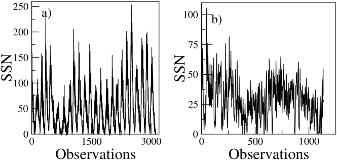
Figure 1.: a) Monthly sunspot record from January 1749 to December 2008. b) Reconstructed sunspot record from Solanki et al. (2004). The time period covers $11\,360$ years with observations in 10-year increments.F-spots

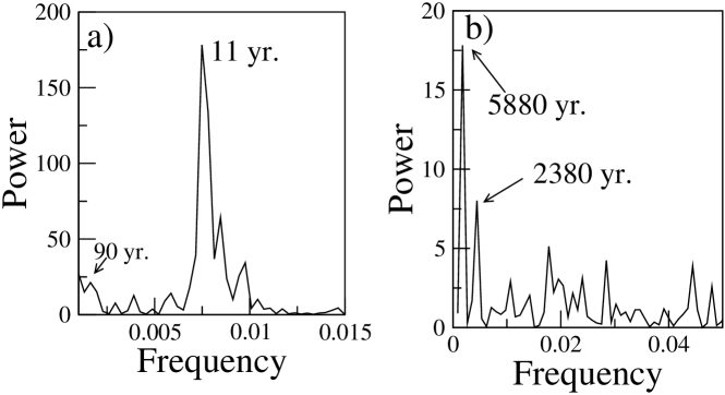
Figure 2.: Power spectra for a) monthly sunspot record from January 1749 to December 2008. b) Reconstructed sunspot record from Solanki et al. (2004). The time period covers $11\,360$ years with observations in 10-year increments.F-spower

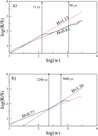
Figure 3.: $\log(R/S)$ vs. $\log(w)$  for sunspot number a) from January 1749 to December 2008 b) reconstructed sunspot record of $11\,360$ years. The Hurst exponents with corresponding standard deviations are a) 1.13$\pm$0.003; 0.83$\pm$0.003 b) 0.77$\pm$0.001; 1.26$\pm$0.004.F-shurst

We further analyze the reconstructed sunspot time series of $11\,360$ years (Solanki et al.2004) shown in Figure F-spots(b). Figure  F-spower(b) shows the power spectrum of this time series indicating the presence of two long-term periodicities at nearly 2300 and 6000 years. The $R/S$ analysis also shows two bendings around these periods (Figure  F-shurst(b)). Again, for this data set we get two linear regimes, the Hurst exponent of the first part being 0.77 and the second part being 1.26.

If we were to calculate a single Hurst exponent for these two time series we will get $H\approx 0.9$ for 259-year and $H\approx 0.8$ for $11\,360$-year data (Figure F-shurst(a) and (b) respectively). These values of the Hurst exponent  agree with the previously estimated values of H in the literature Ruzmaikin, Feynman, and Robinson (1994); Gil-Alana (2009); Xapsos and Burke (2009). However, as we have demonstrated, the log-log plots of sunspot data show two remarkably distinct scaling regimes and hence estimating only one Hurst exponent may be improper. In the next section we examine in detail the reasons for these different scaling regimes by using examples of a variety of time series of standard chaotic systems.

4 Chaotic Models and $R/S$ Analysis

S-resultmodels

In order to understand the behavior of different dynamical systems using the Hurst exponent, we take two extreme examples of time series generated from random and periodic motion respectively. First we take a random time series with $100\,000$ data points distributed uniformly in the range $[0,1]$. Using the $R/S$ method we compute the Hurst exponent as discussed in Section 2 and find the Hurst exponent $H=0.5$ as given by the slope of the line in Figure F-extreme(a), which is expected for a purely random time series Mandelbrot and Wallis (1969a).

We further consider the other extreme case of a purely periodic signal of period one generated from $\sin(x)$, with $x$ in the range $[0,1000]$ with step size $0.01$. Figure F-extreme(b) shows the plot of $\log(R/S)$ vs. $\log(w)$ and the slope of the linear regime in this case is $1$. One prominent difference between these two extreme cases of a purely random signal and a periodic signal (Figure F-extreme(a) and (b) respectively), is that for a purely random signal, the plot of $\log(R/S)$ vs. $\log(w)$ has a constant slope, while for a periodic signal it gets saturated and starts oscillating after a certain value of $w$ (marked by an arrow). The value where the bending begins corresponds to the period of oscillation $T=2\pi/0.01$, and has been verified by the power spectrum. The bending, therefore, gives us information about the frequency of the given signal.

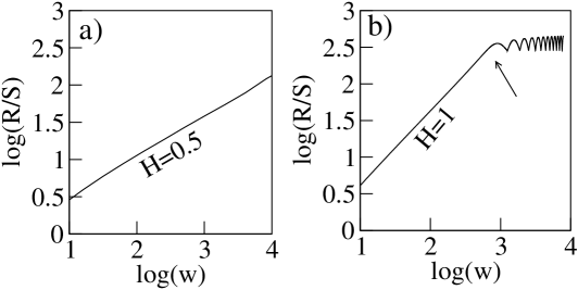
Figure 4.: Plot of $\log(R/S)$ vs. $\log(w)$ for a) random and b) periodic time series.F-extreme

4.1 Chaotic Time Series

In the past few decades, chaotic motion, observed in deterministic systems, has received great attention due to its presence in systems from physical, chemical, biological, ecological, physiological to social sciences. These chaotic motions are temporally aperiodic and are strange because they have a fractal geometry. Since chaotic motion is neither periodic nor random we can expect its behavior to be in-between two extreme cases of randomness and periodicity. Therefore, we can also expect the Hurst exponent to be different from $0.5$ and $1$. An example of a system exhibiting chaotic motion is the celebrated Rössler attractor Rössler (1979),

$$\dot{x} = -y-z,$$

$$\dot{y} = x+ay,$$

$$\dot{z} = b+z(x-c),$$ (2)

where $a$, $b$ and $c$ are control parameters. A chaotic trajectory (with $a=0.1$, $b=0.1$ and $c=18.0$) in the $x-y$ plane is shown in Figure F-single(a) which rotates around an unstable period-one fixed point $((c-d)/2,~{}(-c+d)/{2a},~{}(c-d)/{2a})$ where $d=\sqrt{c^{2}-4ab}$ . The plot of $\log(R/S)$ vs. $\log(w)$ (Figure F-single(c)) shows that there is linear regime (before marked arrow) after which it gets saturated. The slope of linear region gives $H\approx 1$. The first bending of the above-mentioned curve gives the frequency which matches with the frequency obtained from power spectrum or peak to peak analysis of the amplitude. This system is dissipative and has to be bounded in the sub-phase space Rössler (1979) and the bending here corresponds to the folding nature of the dynamics.

In order to see if the behavior is replicated in another similar system, we consider the Chua oscillator (Chua et al., 1993),

$$\dot{x} = c_{1}(y-x-p(x)),$$

$$\dot{y} = c_{2}(x-y+z),$$

$$\dot{z} = -c_{3}y,$$ (3)

where $p(x)$ is defined as,

$$p(x)=m_{1}x+\left((m_{0}-m_{1})(\mid x+1\mid-\mid x-1\mid)\right)/2.$$

We take $c_{1}=15.6$, $c_{2}=1,m_{0}=-8/7,~{}m_{1}=5/7$ and first select the parameter $c_{3}=33$ such that the motion will be a single-scroll type as shown in Figure F-single(b) (there is a symmetric attractor also, depending upon the initial conditions). The $\log(R/S)$ vs. $\log(w)$ plot for variable $x$ is shown in Figure F-single(d) and the Hurst exponent is found to be $H\approx 1$. This also shows saturation at the average time period (shown by arrow). These two examples of chaotic dynamics, Rössler and Chua systems, clearly demonstrate that whenever there is a single center of rotation the $\log(R/S)$ vs. $\log(w)$ plot shows a linear scale only up to the average period of the attractor after which it saturates.

In nature one may come across many dynamical systems which are chaotic and their trajectories rotate around more than one center of rotation. In order to see the behavior of $\log(R/S)$ vs. $\log(w)$ plot, we first consider the Lorenz system Lorenz (1963),

$$\dot{x} = \sigma(y-x),$$

$$\dot{y} = x(\rho-z)-y,$$

$$\dot{z} = xy-\beta z.$$ (4)

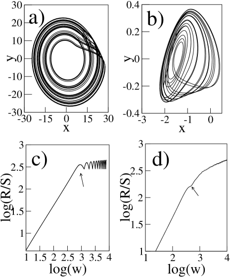
Figure 5.: Plot of trajectories in the $x-y$ plane for chaotic motion of (a) Rössler, b) Chua oscillators having single center of rotation. Corresponding plots of $\log(R/S)$ vs. $\log(w)$ are given in panels c) and d) respectively. F-single

Shown in Figure F-double(a) is the chaotic trajectory in the $x-y$ plane at parameter values $\sigma=16$, $\rho=50$ and $\beta=4$. This clearly shows that the trajectory rotates for some time around the fixed points:

$(\sqrt{\beta\left(\rho-1\right)},\sqrt{\beta\left(\rho-1\right)},\left(\rho-1\right))$ and $(-\sqrt{\beta\left(\rho-1\right)},-\sqrt{\beta\left(\rho-1\right)},\left(\rho-1\right))$,

while some time it rotates around all of these fixed points (including $(0,0,0)$). The $\log(R/S)$ vs. $\log(w)$ plot in Figure F-double(c) shows that there are two regimes of linear scaling. The slope of the first part of the linear region gives $H=0.93$ and the second part gives $H=0.64$. The first linear regime corresponds to the trajectory rotating about individual fixed points while the second is for all three fixed points. This indicates that the dynamics around individual fixed points is different from that of the combined one. Therefore taking the slope of individual regimes can give more details of the intrinsic dynamics. This method also allows us to estimate intrinsic frequencies of the system.

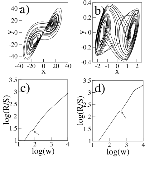
Figure 6.: Plot of trajectories in the $x-y$ plane for chaotic motion of a) Lorenz and b) Chua oscillators having multiple centers of rotation. Corresponding plots of $\log(R/S)$ vs. $\log(w)$ are given in panels c) and d) respectively.F-double

In order to see this behavior in another system where chaotic motion contains many unstable fixed points around which the trajectory revolves, we consider the Chua circuit represented by Equation (eq:chua). Figure F-double(b) shows the trajectory having a double-scroll chaotic motion (Chua system at $c_{3}=28$). Similar to the Lorenz system, this system confirms the existence of two different regimes of linear scaling having the Hurst exponents, $H=1$ and $1.1$. These two examples confirm that for multiple centers of rotation, there are many regimes of linear scaling for which distinct Hurst exponents can be estimated.

5 Conclusions

S-conc

In this paper, we use the Hurst analysis on 259-year and $11\,360$ -year data sets and find multiple Hurst exponents in each time series. We explain the presence of multiple Hurst exponents in a single time series using systems from deterministic chaotic dynamics with a single center of rotation ( Rössler and single-scroll Chua oscillators) as well as multiple centers of rotation (Lorenz and double-scroll Chua oscillators). We have shown that in the sunspot data, two distinct linear scaling regimes exist for which two distinct Hurst exponents could be estimated implying a variety of persistent behavior. The results show very high degree of persistent behavior till 11 years ($H\approx 1.1$), a slightly less persistent behavior till 100 years ($H\approx 0.8$), and comparatively less persistent behavior till 2300 years ($H\approx 0.77$).

Acknowledgements

VS thanks CSIR, India for a Junior Research Fellowship and AP acknowledges DST, India for financial support.

References

- Bray and Loughhead (1979) Bray, R.J., Loughhead, R.E.: 1979, Sunspots, New York, Dover, 256.
- Chua, Itoh, Kocarev, and Ecker (1993) Chua, L.O, Itoh, M., Kocarev, L., Eckert, K.: 1993, J. Circ. Syst. Comput. 3, 1.
- Cohen and Sweetser (1993) Cohen, T.J, Sweetser, E.I.: 1975, Nature 256, 295.
- Cole (1973) Cole, T.W.: 1973, Solar Phys. 30, 103.
- Eddy (1976) Eddy, J.: 1976, Science 192, 1189.
- Gil-Alana (2009) Gil-Alana, L.A.: 2009, Solar Phys. 257, 371.
- Kilcik, Anderson, and Rozelot (2009) Kilcik, A., Anderson, C.N.K., Rozelot, J.P., Ye, H., Sugihara, G., Ozguc, A.: 2009, Astrophys. J. 693, 1173.
- Kimura (1913) Kimura, H.: 1913, Mon. Not. Roy. Astron. Soc. 73, 543.
- Kiral (1961) Kiral, A.: 1961, Publ. Istanbul Univ. Observ. 70.
- Lorenz (1963) Lorenz, E.N.: 1963, J. Atmos. Sci. 20, 130.
- Mandelbrot and Wallis (1969a) Mandelbrot, B., Wallis, J.R.: 1969a, Water Resour. Res.. 5, 228.
- Mandelbrot and Wallis (1969) Mandelbrot, B., Wallis, J.R.: 1969b, Water Resour. Res.. 5, 967.
- Michelson (1913) Michelson, A.A.: 1913, Astrophys. J. 38, 268.
- Rössler (1979) Rössler, O.E.: 1979, Phys. Rev. Lett. 71A, 155.
- Ruzmaikin (1981) Ruzmaikin, A.A.: 1981, Comments Astrophys. 9, 85.
- Ruzmaikin, Feynman, and Robinson (1994) Ruzmaikin, A., Feynman, J., Robinson, P.: 1994, Solar Phys. 148, 395.
- (17) Schwabe, S.H.: 1843, Astron. Nachr. 20, 234.
- Solanki, Usoskin, Kromer, Schussler, and Beer (2004) Solanki, S.K., Usoskin, I.G., Kromer, B., Schussler, M., Beer, J.: 2004, Nature 431,1084.
- Theiler (1986) Theiler, J.: 1986, Phys. Rev. A34,2427.
- Turner (1913) Turner, H.H: 1913, Mon. Not. Roy. Astron. Soc. 73, 549.
- Wittmann (1978) Wittmann, A.: 1978, A&A66, 93.
- Xapsos and Burke (2009) Xapsos, M.A, Burke, E.A.: 2009, Solar Phys. 257, 363.
- Zhukov and Muzalevskii (1969) Zhukov, L.V., Muzalevskii, Y.S.: 1969, Astron. Zh. 46, 600 (Soviet Astron. 13, 473).