Stochastic Load-Redistribution Model for Cascading Failure Propagation

Abstract

A new class of probabilistic models for cascading failure propagation in interconnected systems is proposed. The models are able to represent important physical characteristics of realistic load-redistribution mechanisms, e.g., that the load increments after a failure depend on the load of the failing element and that they may be distributed non-uniformly among the remaining elements. In the limit of large system sizes, the models are solved analytically in terms of generalized branching processes, and the failure propagation properties of a prototype example are analyzed in detail.

I Introduction

The increasing complexity of today’s infrastructure networks, e.g., electrical power grids, road systems, or communication networks, makes them very sensitive to local failures Motter2002 ; Watts2002 ; Dobson2007 ; Simonsen2008 ; Buldyrev2009 . When an element in such a network fails, its “load” (e.g., power, traffic, or information flow) is redistributed to the other elements of the network. Some of the increased loads may then exceed the capacity of their respective element, leading to further failures and eventually to a cascading breakdown of the entire network. Cascading failure propagation is not only observed in physical infrastructure networks, but also in social and economic systems Motter2002 ; Watts2002 or in the fracture of heterogeneous materials Alava2006 ; Pradhan2008 .

As a breakdown of critical infrastructure networks can have serious economic consequences, it is crucial to gain a deeper understanding of the mechanisms that lead to such cascading failures. This problem has, in particular, attracted the interest of the statistical physics community, and various models have been developed to study the vulnerability of complex networks with respect to cascading failure propagation Motter2002 ; Watts2002 ; Dobson2007 ; Bakke2006 ; Simonsen2008 . A description of the load-redistribution on different levels of detail has been considered, e.g., more physical approaches based on resistor networks Bakke2006 or complex-network models focusing on purely topological measures like the betweenness centrality Motter2002 ; Albert2004 ; Huang2008 . The dynamics of most of these models, however, can only be analyzed via large-scale numerical simulations. In order to obtain an analytically solvable model, Dobson et al. Dobson2007 ; Dobson2005 consider the simplifying assumption that the load increments after a failure are the same for all remaining elements and independent of the failing load. Similarly, fiber bundle models for the problem of fracture propagation Daniels1945 ; Alava2006 ; Pradhan2008 ; Hidalgo2002 can only be solved analytically if the load of the failing fiber is equally redistributed to all remaining fibers.

In this paper, we introduce and analyze a new class of probabilistic models for cascading failure propagation that can represent, in a stochastic sense, important characteristics of realistic load-redistribution mechanisms: The load redistribution after a failure is no longer assumed to be uniform and the induced load increments may depend on the load of the failing element. With such models, we can thus expect to obtain a better understanding of the breakdown processes in real networks. We show that in the limit of large system sizes, our models can be solved analytically by using a Markov approximation and the theory of generalized branching processes Harris1963 . We then apply our general approach to an illustrative prototype system that roughly imitates failure propagation in a power transmission network and analyze its vulnerability with respect to cascading breakdown.

II Cascading-failure model

We consider a system consisting of $N$ elements, each with a random load $L\geq 0$. The loads are assumed to be independent of each other and identically distributed. Furthermore, every element possesses a random critical load $L^{\mathrm{max}}$ above which it will fail. Whereas we assume that the critical loads of the various elements are independent of each other, we allow for possible correlations between the initial and critical loads of a particular element. Specifically, we require that initially none of the elements is overloaded, i.e., the probability $P(L>L^{\mathrm{max}})$ vanishes.

We now consider a situation where, due to some external influence, one of the elements, say with load $L_{\mathrm{f}}$, fails. Our central model assumption is that this load is redistributed to the remaining elements according to the stochastic load-redistribution rule

$$L\rightarrow L^{\prime}=L+L_{\mathrm{f}}\,\Delta\,.$$ (1)

Here, $L$ ($L^{\prime}$) is the load of one of the remaining elements before (after) failure of the element with load $L_{\mathrm{f}}$, and the load-redistribution factor $\Delta$ is a random number drawn independently from the same distribution for each of the remaining elements. In other words: The load increments are proportional to the failed load $L_{\mathrm{f}}$, but with random proportionality factors $\Delta$.

The form of rule (1) is based on the observation that in many systems, the load-redistribution factors primarily depend on structural properties, such as interactions between the various elements, and not on the load of the failing element. In a more “microscopic” approach, the failure dynamics of such systems would be described by a model of the form (1), but with the factor $\Delta$ being determined by the specific interactions of the failing element with the one affected by the failure. Corresponding examples range from the power-flow redistribution after a line failure in power grids Baldick2003 to the distance-dependent stress redistribution in fiber bundles Hidalgo2002 . The main features of a load redistribution of the form (1) can already be understood by considering the extreme cases of a uniform, global load redistribution and a purely local one. In the former case, each element is affected in the same way and thus $\Delta=1/(N-1)$. The latter situation is described by $\Delta=1/Z$ for the $Z$ nearest neighbors of the failing element and zero otherwise. The stochastic load redistribution rule (1) models the microscopic $\Delta$-dependence in terms of a noisy dynamics that neglects any spatial correlations. While its specific form thus depends on the system at hand—we will consider an example in Sect. IV below—we expect two properties to be generally fulfilled: (i) On average, the failed load will be redistributed to the remaining $N-1$ elements. This implies that the mean $\langle\Delta\rangle$ behaves as $1/N$ for large $N$. (ii) The $\Delta$-distribution typically will be bounded. For instance, if—in the worst case—one single element has to take over the load of the failing element, one has $|\Delta|\leq 1$.

So far, we have only discussed the load redistribution after an initial failure. Obviously, it can happen that the post-failure loads of a number $N_{\mathrm{f}}^{(1)}\geq 1$ of elements are above their respective critical loads. In such a situation, a failure cascade develops. For its description, we assume that the overloaded elements fail simultaneously and that each failing load is redistributed to the remaining elements according to rule (1) . If this redistribution results in further overloading, the cascade continues to a new cascade stage. This process continues until the system either reaches a stable state, i.e., the remaining elements operate within their bounds, or all $N$ elements have failed and the system has broken down completely.

Denoting the number of failures at each cascade stage $s=1,2,\dots$ by $N_{\mathrm{f}}^{(s)}$ and counting the initial failure as $N_{\mathrm{f}}^{(0)}=1$, the total number of failed elements $N_{\mathrm{f}}=\sum_{s=0}N_{\mathrm{f}}^{(s)}$ provides a measure for the damage to the system. The distribution of this random variable characterizes the system stability. Coarsely, two regimes can be distinguished: (i) The probability of large $N_{\mathrm{f}}$ decays quickly, i.e., at least exponentially, and thus system-wide cascades with $N_{\mathrm{f}}\lesssim N$ constitute very rare events; (ii) System-wide failures occur with finite probability even for $N\to\infty$. At the separation between these two regimes, the system exhibits a “critical” behavior Dobson2007 , where large-scale events are still suppressed but their probability only decays according to a power law: $P(N_{\mathrm{f}})\propto N_{\mathrm{f}}^{-\gamma}$ for $N\to\infty$.

To determine the stability of a given system with respect to cascading failures, the detailed form of the probability distribution $P(N_{\mathrm{f}})$ is not required and will not be evaluated in the present paper. Instead, it suffices to have an indicator for the two regimes just outlined. An obvious choice is the probability for a system-wide breakdown: $P_{\mathrm{b}}=P(N_{\mathrm{f}}=N)$. Another quantity of interest is the probability that an initial failure does not induce any further failures, in other words, the probability that no cascade develops at all: $P_{\mathrm{nc}}=P(N_{\mathrm{f}}=1)$

III Generalized-branching-process approximation

In the limit of large systems, $N\to\infty$, when finite-size effects do not play a role, an approximate description of the cascade dynamics can be obtained by making two observations: First, during a failure cascade, the distribution of the not yet failed loads can be approximated by their initial distribution. Thus, a Markovian description in terms of the loads which fail at every cascade step becomes possible. The corresponding states form a point process on the non-negative real axis van_Kampen2007 . Second, as the number of remaining elements always stays infinitely large, the number of induced failures can be described by a Poisson distribution. This yields an approximation of our model in terms of a generalized branching process Harris1963 , which is fully defined by its characteristic functional

$$\begin{split}G[u;L_{\mathrm{f}}]=\exp\bigg{\{}\mu_{\mathrm{f}}(L_{\mathrm{f}})\bigg{[}\int\!&\mathrm{d}L_{\mathrm{f}}^{\prime}\,\,p(L_{\mathrm{f}}^{\prime}|L_{\mathrm{f}}^{\prime}>L^{\mathrm{max}};L_{\mathrm{f}})\\ &\times\mathrm{e}^{-u(L_{\mathrm{f}}^{\prime})}-1\bigg{]}\bigg{\}}\,,\end{split}$$ (2)

where $u$ denotes an arbitrary non-negative test function on the interval $[0,\infty)$ and $p(L_{\mathrm{f}}^{\prime}|L_{\mathrm{f}}^{\prime}>L^{\mathrm{max}};L_{\mathrm{f}})$ is the conditional probability density that a failure induced by a failing load $L_{\mathrm{f}}$ occurs with a load $L_{\mathrm{f}}^{\prime}$. Given the joint distribution of initial and critical loads, as well as the distribution of the load-redistribution factors, this quantity can be readily calculated. The mean number of induced failures is given by $\mu_{\mathrm{f}}(L_{\mathrm{f}})=(N-1)\,P(L_{\mathrm{f}}^{\prime}>L^{\mathrm{max}}|L_{\mathrm{f}})$. Note that in order for a meaningful limit $N\to\infty$ to exist this implies that the conditional failure probability of a single element $P(L_{\mathrm{f}}^{\prime}>L^{\mathrm{max}}|L_{\mathrm{f}})$ has to be of order $O(1/N)$ (cf. the discussion above on the mean of the load-redistribution factors).

For the calculation of the breakdown and no-cascade probabilities, we condition these quantities on the load $L_{\mathrm{f}}$ of the failing element. From the Poissonian distribution of the failures induced directly by this initial failure, one then obtains the conditional no-cascade probability $P_{\mathrm{nc}}(L_{\mathrm{f}})=\exp[-\mu_{\mathrm{f}}(L_{\mathrm{f}})]$. The conditional breakdown probability $P_{\mathrm{b}}(L_{\mathrm{f}})$ can be obtained as solution of the integral equation Harris1963

$$1-P_{\mathrm{b}}(L_{\mathrm{f}})=\exp\bigg{\{}-\mu_{\mathrm{f}}(L_{\mathrm{f}})\int\!\mathrm{d}L_{\mathrm{f}}^{\prime}\,\,p(L_{\mathrm{f}}^{\prime}|L_{\mathrm{f}}^{\prime}>L^{\mathrm{max}};L_{\mathrm{f}})\\ \times P_{\mathrm{b}}(L_{\mathrm{f}}^{\prime})\bigg{\}}\,.$$ (3)

This relation can be interpreted in the sense that the probability that no complete breakdown develops after a failure with load  $L_{\mathrm{f}}$ equals the probability that—in the limit $N\to\infty$—none of the induced failures with load $L_{\mathrm{f}}^{\prime}$ leads to a breakdown. Starting from an initial guess for $P_{\mathrm{b}}(L_{\mathrm{f}})$, Eq. (3) can be efficiently solved by means of an iterative procedure Harris1963 . This either yields the vanishing solution $P_{\mathrm{b}}(L_{\mathrm{f}})\equiv 0$ if the system is immune against cascading failures or the unique nontrivial solution with finite breakdown probability. Note that the range of possible $L_{\mathrm{f}}$ in Eq. (3) might be larger than that of the initial loads $L$ (see the example in Sect. IV below). We finally remark that an integral relation similar to Eq. (3) can be derived for the generating function of the total number of failures $N_{\mathrm{f}}(L_{\mathrm{f}})$, where $L_{\mathrm{f}}$ is the initially failing load.

IV Example: Simple bimodal load redistribution

As a simple, yet prototypical example, we now consider a bimodal load redistribution:

$$\Delta=\begin{cases}\Delta_{0}&\text{with probability ${p_{0}}$}\\ 0&\text{with probability $1-{p_{0}}$}\,.\end{cases}$$ (4)

Thus, a failure affects a specific other element with probability ${p_{0}}$, in which case this element receives a portion $\Delta_{0}$ of the failed load. In line with the above arguments, we require $\langle\Delta\rangle={p_{0}}\,\Delta_{0}=1/(N-1)$ and consequently $1/(N-1)\leq\Delta_{0}\leq 1$. On average, the failing load is redistributed to $(N-1){p_{0}}=1/\Delta_{0}$ other elements. In this sense, the model allows one to study the transition between the above-mentioned two extreme cases of a global load redistribution for $\Delta_{0}=1/(N-1)$ and a load transfer to a single other element, typically the nearest neighbor, for $\Delta_{0}=1$.

For the initial loads $L$, we consider a uniform distribution, which can be scaled without loss of generality to the interval $[0,1]$. Motivated by applications to infrastructure networks with cost-limited capacity, e.g., power transmission networks, we assume that the maximal load of each element is higher than its initial load by a constant tolerance $\alpha\geq 0$ Motter2002 :

$$L^{\mathrm{max}}=(1+\alpha)\,L\,.$$ (5)

In the limit $N\to\infty$, the model is thus fully characterized by the two parameters $\Delta_{0}$ and $\alpha$ and in the following, we shall study the stability of the system as a function of these parameters.

As shown above, the no-cascade probability $P_{\mathrm{nc}}$ follows directly from the mean number of failures induced by a failure with load $L_{\mathrm{f}}$. From $P(L_{\mathrm{f}}^{\prime}>L^{\mathrm{max}}|L_{\mathrm{f}})={p_{0}}\,P(L<L_{\mathrm{f}}\,\Delta_{0}/\alpha)$, where $L$ is the initial load of an arbitrary element, we obtain $\mu_{\mathrm{f}}(L_{\mathrm{f}})=\min(1/\Delta_{0},L_{\mathrm{f}}/\alpha)$. The integral equation (3) for the conditonal breakdown probability $P_{\mathrm{b}}(L_{\mathrm{f}})$ assumes the form

$$1-P_{\mathrm{b}}(L_{\mathrm{f}})=\exp\bigg{\{}-\frac{1}{\Delta_{0}}\!\!\!\!\int\limits_{L_{\mathrm{f}}\Delta_{0}}^{L_{\mathrm{f}}\Delta_{0}+\min(1,L_{\mathrm{f}}\Delta_{0}/\alpha)}\!\!\!\!\!\!\!\!\!\!\!\!\!\!\!\!\!\!\!\!\!\mathrm{d}L_{\mathrm{f}}^{\prime}\,\,P_{\mathrm{b}}(L_{\mathrm{f}}^{\prime})\bigg{\}}\,.$$ (6)

It has to be solved on the interval $[0,L_{\mathrm{f,max}}]$ with $L_{\mathrm{f,max}}=1/(1-\Delta_{0})$ for $\alpha<\Delta_{0}/(1-\Delta_{0})$ and $L_{\mathrm{f,max}}=1$ otherwise.

If we assume that the initially failing element is chosen at random with equal probability, we obtain the total no-cascade and breakdown probabilities, $P_{\mathrm{nc}}$ and $P_{\mathrm{b}}$, respectively, by integrating the corresponding conditioned probabilities over the range $[0,1]$ of possible initially failing loads. Whereas for the breakdown probability, the integral has to be performed numerically from the iterative solution of Eq. (6), the no-cascade probability can be obtained explicitly:

$$P_{\mathrm{nc}}=\begin{cases}\alpha+(1-\alpha-\alpha/\Delta_{0})\,\mathrm{e}^{-1/\Delta_{0}}&\!\!\text{for $\alpha<\Delta_{0}$}\\ \alpha-\alpha\,\mathrm{e}^{-1/\alpha}&\!\!\text{for $\alpha\geq\Delta_{0}$}.\end{cases}$$ (7)

Figure 1 shows the probabilities $P_{\mathrm{nc}}$ and $P_{\mathrm{b}}$ as a function of the tolerance $\alpha$ for various values of the redistribution factor $\Delta_{0}$.

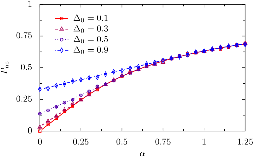
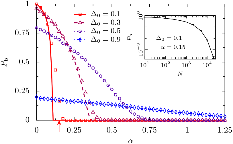
Figure 1: No-cascade (upper panel) and breakdown (lower panel) probabilities, $P_{\mathrm{nc}}$ and $P_{\mathrm{b}}$, respectively, as a function of the tolerance $\alpha$ for different values of the load-redistribution parameter $\Delta_{0}$. Lines: Eq. (7) (upper panel) and results from an iterative solution of Eq. (6) (lower panel). Symbols: Monte-Carlo results from a simulation of the stochastic dynamics (1) for $N=2000$ elements and $10^{4}$ realizations. The statistical error is below the size of the symbols. Inset of lower panel: Monte-Carlo results (from $10^{5}$ realizations) as a function of the system size $N$ for $\Delta_{0}=0.1$ and $\alpha=0.15$, as indicated by the arrow in the lower panel. The line serves as a guide to the eye.

We observe (see upper panel) that the no-cascade probability $P_{\mathrm{nc}}$ gradually increases from its minimal value $\exp(-1/\Delta_{0})$ for $\alpha=0$ but remains considerably below one over the considered $\alpha$-range. This is in stark contrast to the behavior of the breakdown probability (see lower panel), which decreases with increasing tolerance $\alpha$ to vanish completely above a certain critical $\alpha$-value. In this latter regime, the system becomes stable in the sense that cascading failures affecting it as a whole do not occur with finite probability. With increasing load-redistribution factor $\Delta_{0}$, the transition to this regime happens at higher $\alpha$-values and also becomes less sharp. Comparing with the no-cascade probabilities $P_{\mathrm{nc}}$, we find that those cannot serve as a reliable indicator for the system stability: Consider, for example, the case $\alpha=0.5$, where the breakdown probability varies strongly with $\Delta_{0}$, as opposed to the no-cascade probability, which is even independent of $\Delta_{0}$ for $\Delta_{0}\leq\alpha$.

In Fig. 1, we also compare the results from the generalized-branching-process approximation with those obtained from a Monte-Carlo simulation of the full stochastic dynamics (1) for a system consisting of $N=2000$ elements (see symbols in Fig. 1). Within the statistical error, we find a very good agreement, except near the transition to a stable system in the case of small load-redistribution factors $\Delta_{0}$. In this regime, the failing load is distributed to a large number of elements, but not all of them fail immediately. Their increased load, however, will eventually lead to a higher breakdown probability than predicted by the branching-process approximation, where this effect is neglected. As the number of such elements is independent of the system size, this finite-size effect will vanish in the limit of very large systems. As shown exemplarily for the case $\Delta_{0}=0.1$ and $\alpha=0.15$ in the inset of Fig. 1, the breakdown probability obtained from Monte-Carlo simulations indeed approaches zero with increasing system size $N$, in agreement with the solution obtained from Eq. (6).

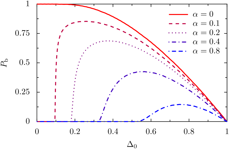
Figure 2: Breakdown robability $P_{\mathrm{b}}$ obtained from an iterative solution of Eq. (6) as a function of the load-redistribution parameter $\Delta_{0}$ for different values of the element tolerance $\alpha$.

It is also interesting to look at the behavior of the breakdown probability as a function of the load-redistribution factor $\Delta_{0}$ (see Fig. 2). For a fixed tolerance $\alpha$, we find a vanishing breakdown probability $P_{\mathrm{b}}$ for small $\Delta_{0}$, which corresponds to “well-connected” systems where the failing load is redistributed to a large number of other elements. Above a critical $\Delta_{0}$-value, the breakdown probability increases abruptly, in particular for small tolerances $\alpha$. It reaches a maximum and then gradually decreases again towards zero in the limit of $\Delta_{0}$ going to unity, where the failing load is transferred to a single other element. It follows that the network is robust against cascading breakdown if $\Delta_{0}$ is smaller than its $\alpha$-dependent critical value.

Finally, we compare our results with those of a simple branching process model, e.g., Refs. Dobson2007 ; Dobson2005 , where the induced load increments are independent of the load of the failing element. In these models, the no-cascade probability $P_{\mathrm{nc}}$ as well as the breakdown probability $P_{\mathrm{b}}$ are completely determined by a single quantity, the mean number $\mu_{\mathrm{f}}$ of failures that are induced by a failing element. In particular, $P_{\mathrm{b}}$ is zero if $\mu_{\mathrm{f}}<1$ and finite if $\mu_{\mathrm{f}}>1$. When such a model is applied to our prototype example, the load increments after a failure are equal to a constant $Q_{0}$ with probability $p_{0}$ and zero otherwise. It follows that $\mu_{\mathrm{f}}=\min(1/2\alpha,1/2Q_{0})$, and we note that for a consistent comparison with our model, $Q_{0}$ has to be identified with $\Delta_{0}/2$. As a function of $\alpha$, the breakdown probability $P_{\mathrm{b}}$ then becomes zero at the critical value $\alpha_{\mathrm{c}}=1/2$, which is independent of the value of $\Delta_{0}$. In contrast to our results of Fig. 2, we thus find that such a model does not exhibit a critical behavior with respect to the parameter $\Delta_{0}$, i.e., the breakdown probability stays finite for arbitrarily small values of $\Delta_{0}$ if $\alpha<1/2$. For $\alpha\geq 1/2$, $P_{\mathrm{b}}$ is zero for all values of $\Delta_{0}$ ($0\leq\Delta_{0}\leq 1$).

V Conclusions

We have introduced and analyzed a class of stochastic failure-propagation models which, compared to previous approaches, enable a more realistic description of real systems, while still being amenable to an analytical treatment. The approach is applied to a prototype example that is motivated by the propagation of line failures in power transmission networks. The initial loads (power flows) have random values and the maximum load an element can carry is assumed to be equal to $(1+\alpha)$ times its initial load, Eq. (5). With this example, we have demonstrated that our model not only exhibits a critical behavior as a function of the failure tolerance $\alpha$, but also with respect to a parameter $\Delta_{0}$ that characterizes the variance of the load-redistribution factors and thus depends on physical as well as on topological properties of the load or flow dynamics.

While our assumption of stochastic load redistribution neglects any spatial correlations, we are still able to gain new insights into the vulnerability of complex networks. If we use a more realistic distribution of redistribution factors $\Delta$, our results on the critical behavior of the breakdown probability with respect to failure tolerance and “connectivity”, e.g., may give valuable information for the design of more robust infrastructure systems.

Finally, we note that our models can not only be applied to critical infrastructure networks, but also to other breakdown phenomena, e.g., to failure propagation in elastic fiber bundles Alava2006 ; Pradhan2008 . Within our approach, a corresponding model (with stochastic load redistribution) is obtained if we assume that the initial loads are all identical and that the critical loads of the individual elements are randomly distributed. A detailed study of such models will be presented in a separate publication Lehmann2010 .

References

- (1) A. E. Motter and Y. Lai, Phys. Rev. E 66, 065102(R) (2002).
- (2) D. J. Watts, Proc. Natl. Acad. Sci. U.S.A. 99, 5766 (2002).
- (3) I. Dobson, B. A. Carreras, V. E. Lynch, and D. E. Newman, Chaos 17, 026103 (2007).
- (4) I. Simonsen, L. Buzna, K. Peters, S. Bornholdt, and D. Helbing, Phys. Rev. Lett. 100, 218701 (2008).
- (5) S. V. Buldyrev, R. Parshani, G. Paul, H. E. Stanley, and S. Havlin, arXiv:0907.1182 (2009).
- (6) M. J. Alava, P. K. V. V. Nukala, and S. Zapperi, Adv. Phys. 55, 349 (2006).
- (7) S. Pradhan, A. Hansen, and B. K. Chakrabarti, arXiv:0808.1375 (2008).
- (8) J. Ø. H. Bakke, A. Hansen, and J. Kertész, Europhys. Lett. 76, 717 (2006).
- (9) R. Albert, I. Albert, and G. L. Nakarado, Phys. Rev. E 69, 025103(R) (2004).
- (10) L. Huang, Y.-C. Lai, and G. Chen, Phys. Rev. E 78, 036116 (2008).
- (11) I. Dobson, B. A. Carreras, and D. E. Newman, Prob. Eng. Inf. Sci. 19, 15 (2005).
- (12) H. E. Daniels, Proc. R. Soc. Lond. A, 183, 405 (1945).
- (13) R. C. Hidalgo, Y. Moreno, F. Kun, and H. J. Herrmann, Phys. Rev. E 65, 046148 (2002).
- (14) T. E. Harris, The Theory of Branching Processes, Vol. 119 of Die Grundlehren der Mathematischen Wissenschaften (Springer, Berlin, 1963).
- (15) N. G. van Kampen, Stochastic Processes in Physics and Chemistry, 3rd ed. (Elsevier, Amsterdam, 2007).
- (16) R. Baldick, IEEE Trans. Power Syst. 18, 1316 (2003).
- (17) J. Lehmann and J. Bernasconi, to be published.