Quantum dice rolling: A multi-outcome generalization of quantum coin flipping

Abstract

We generalize the problem of coin flipping to more than two outcomes and parties. We term this problem dice rolling, and study both its weak and strong variants. We prove by construction that in quantum settings (i) weak $N$-sided dice rolling admits an arbitrarily small bias for any value of $N$, and (ii) two-party strong $N$-sided dice rolling saturates the corresponding generalization of Kitaev’s bound for any value of $N$. In addition, we make use of this last result to introduce a family of optimal $2m$-party strong $n^{m}$-sided dice rolling protocols for any value of $m$ and $n$.

I Introduction

Coin flipping (CF) is a cryptographic problem in which a pair of remote distrustful parties, usually referred to as Alice and Bob, must generate a random bit that they agree on. There are two types of coin flipping protocols. In weak CF one of the parties prefers one of the outcomes and the other prefers the opposite, whereas in strong CF each party does not know the other’s preference. The security of a CF protocol is quantified by the biases $\epsilon_{A}^{\left(i\right)}$ and $\epsilon_{B}^{\left(i\right)}$ ($i=0,\,1$); if $\left.P_{A}^{\left(i\right)}\right.^{*}$ and $\left.P_{B}^{\left(i\right)}\right.^{*}$ are the maximal probabilities that a dishonest Alice or Bob can force the outcome $i$, then

$$\epsilon_{j}^{\left(i\right)}\hat{=}\left.P_{j}^{\left(i\right)}\right.^{*}-\frac{1}{2}\,,\qquad i\in\left\{0,\,1\right\}\,.$$ (1)

The biases tell us to what extent each of the parties can increase beyond one half their chances of obtaining each of the outcomes. In weak CF we associate each of the outcomes with a win of one party over the other. Hence, we are not interested in bounding the maximal losing probability and we consequently consider only two biases: $\epsilon_{i}\hat{=}P_{i}^{*}-1/2$, where $P_{i}^{*}$ is dishonest party $i$’s maximal winning probability. $\epsilon\hat{=}\max\left(\epsilon_{A},\,\epsilon_{B}\right)$, or $\epsilon\hat{=}\max\bigl{(}\epsilon_{A}^{\left(0\right)},\,\epsilon_{A}^{\left(1\right)},\,\epsilon_{B}^{\left(0\right)},\,\epsilon_{B}^{\left(1\right)}\bigr{)}$ in the case of strong CF, is often referred to as the bias of the protocol.

The problem of CF was first introduced by Blum in 1981, who analyzed it in classical settings Blum . It was subsequently shown that if there are no limitations on the parties’ computational power a dishonest party can always force any outcome they desire Kilian . With the publication of the quantum key distribution protocol of Bennett and Brassard in 1984 BB84 , it was realized that many communication tasks that are impossible in a classical setting may be possible in a quantum setting. In 1999 Goldenberg et al. introduced a quantum gambling protocol Gambling , which is a problem closely related to weak CF (see footnote ). The first quantum (strong) coin flipping protocol per se was presented by Aharonov et al. in 2000 Aharonov . The protocol achieves a bias of $\sqrt{2}/4\simeq 0.354$ Spekkens -2 . Soon afterward Spekkens and Rudolph Spekkens -1 , and independently Ambainis Ambainis , devised a strong CF protocol with a bias of $1/4$. On the other hand, Kitaev subsequently proved that there is a limit to the efficacy of strong CF protocols Kitaev : Any strong CF protocol must satisfy $\left.P_{A}^{\left(i\right)}\right.^{*}\cdot\left.P_{B}^{\left(i\right)}\right.^{*}\geq 1/2$, $i\in\left\{0,\,1\right\}$. As regards weak CF, in 2002 Spekkens and Rudolph introduced a family of three rounds of communication protocols in which both dishonest parties have a bias of $(\sqrt{2}-1)/2\simeq 0.207$ Spekkens . Mochon then improved upon Spekkens and Rudolph’s result by constructing weak CF protocols with an infinite number of rounds Mochon_-2 ; Mochon_-1 . These efforts culminated in a proof that weak CF with an arbitrarily small bias is possible Mochon . Most recently, building upon Mochon’s latest result, Chailloux and Kerenidis devised a strong CF protocol, which saturates Kitaev’s bound in the limit of an infinite number of rounds Kerenidis .

CF admits many generalizations. We may consider imbalanced coins, more than two outcomes, more than two parties, or indeed some or all of these possibilities combined. An analysis of multi-party strong CF – the problem of $N$ remote distrustful parties having to decide on a bit – in quantum settings was carried out in Multi-party , and similarly to the two-party case, it was shown that the use of quantum resources is advantageous. Even though it is usually mentioned only with respect to the balanced case, the general statement of Kitaev’s bound reads

$$\left.P_{A}^{\left(i\right)}\right.^{*}\cdot\left.P_{B}^{\left(i\right)}\right.^{*}\geq P_{i}\,,\qquad i\in\left\{0,\,1\right\}\,,$$ (2)

where $P_{i}$ is the probability of the outcome $i$ in an honest execution of the protocol. One of the results of this paper is the generalization of Chailloux and Kerenidis’ optimal Strong CF protocol to cover the imbalanced case as well. Similalry, also in the weak case, optimal protocols exist for every degree of imbalance Kerenidis , thereby generalizing Mochon’s aforementioned result.

Somewhat surprisingly, CF has yet to be generalized to many outcomes. Indeed, even in classical settings this problem is nontrivial, as a dishonest party can no longer force with certainty all of the outcomes. In this paper we shall focus on two problems. In the first, which we term weak dice rolling (DR), $N>2$ remote distrustful parties must agree on a number between $1$ and $N$ with party $i$ preferring the $i$-th outcome. In the second, which we term strong DR, $M$ remote distrustful parties must agree on a number between $1$ and $N$ without any party being aware of any other’s preference.

The paper is organized as follows. In section II we prove that, using quantum resources, weak $N$-sided dice rolling with arbitrarily small bias is possible for any value of $N$. This result stands in marked contrast to the classical case, where, under certain conditions, an honest party always loses. Furthermore, to gain insight as to what biases are achievable with a minimal number of rounds of communication, we present a six-round weak three-sided DR protocol, which incorporates a three-round weak imbalanced CF protocol that generalizes the results of Spekkens and Rudolph to the imbalanced case. In section III we generalize Kitaev’s bound to any number of parties, $M$, and outcomes, $N$, and present a family of two-party protocols that saturate it for any value of $N$. We then make use of this family to extend this result to $2m$-party $n^{m}$-sided DR any for value of $m$ and $n$. In the process, we generalize Chailloux and Kerenidis’ optimal strong CF protocol to cover the imbalanced case. Finally, we analyze a family of three-round two-party strong $N$-sided DR protocols for any value of $N$.

II Weak dice rolling with arbitrarily small bias

The purpose of weak CF is to decide between two parties. Hence, its natural multi-outcome generalization is the problem of deciding between $N>2$ parties. As opposed to weak CF, in weak $N>2$-sided DR there are many different cheating scenarios, as any number of parties $n<N$ may be dishonest. We shall be interested in the $N$ “worst case” scenarios where all but one of the parties are dishonest and, moreover, are acting in unison. That is, the dishonest parties share classical and quantum communication channels and have a joint strategy. In addition, we shall require that the protocol be “fair” in the sense that the honest party’s maximum losing probability be the same in each of these $N$ scenarios. Of course, the security of the protocol can be evaluated with respect to any other cheating scenario, but as we shall consider only fair protocols, the security of any cheating scenarios is never poorer than that provided by the afore-mentioned $N$ worst case scenarios.

We begin by observing that in CF the bias has a complementary definition. Concentrating on weak CF, we could just as well define it as

$$\bar{\epsilon}_{i}\hat{=}\bar{P}_{i}^{*}-1/2\,,\qquad i=A,\,B$$ (3)

where $\bar{P}_{i}^{*}=P_{j\neq i}^{*}$ is the maximum probability that party $i$ loses. According to this definition the bias tells us to what extent party $j\neq i$ can increase other party $i$’s chances of losing beyond one half. In the case of $N$ parties, the bias $\bar{\epsilon}_{i}$ then tells us to what extent the $N-1$ dishonest parties can increase party $i$’s chances of losing beyond $1-1/N$, rather than to what extent a sole dishonest party can increase its chances of winning beyond $1/N$. We shall always use this redefinition of the bias when considering weak DR. The computation of biases in weak DR is therefore equivalent to the computation of biases in a weak imbalanced coin flipping protocol.

II.1 Weak dice rolling with arbitrarily small bias

We shall now prove that quantum weak $N$-sided DR with arbitrarily small bias is possible for any $N$. The proof is by construction. Consider the following $N$-party protocol. Each party is uniquely identified according to a number from $1$ to $N$. The protocol consists of $N-1$ stages. In stage one parties $1$ and 2 “weakly flip” a balanced quantum coin. The winner and party $3$ then weakly flip an imbalanced quantum coin in stage two, where if both parties are honest $3$’s winning probability equals $1/3$. And so on, the rule being that in stage $n\geq 2$ the winner of stage $n-1$ and party $n$ “weakly flip” an imbalanced quantum coin, where if both parties are honest, $n$’s winning probability equals $1/\left(n+1\right)$. Thus, if all parties are honest each has the same overall winning probability of $1/N$. Using Mochon’s formalism Mochon , Chailloux and Kerenidis have recently proved that weak imbalanced coin flipping with arbitrarily small bias is possible Kerenidis . It follows that in the limit where each of the weak imbalanced coin flipping protocols, used to implement our DR protocol, admits a vanishing bias (and $N$ is finite), any honest party’s winning probability tends to $1/N$; for a formal proof see appendix A. Moreover, since we have considered the worst case cheating scenario, this result holds for any other cheating scenario.

The above result stands in stark contrast to the classical case where if the number of honest parties is not strictly greater than $N/2$, then the dishonest parties can force any outcome they desire. To see why this is so, let us consider a classical $N$-sided dice rolling protocol and partition the parties into two groups of $m\leq\left\lceil N/2\right\rceil$ and $n=N-m$ parties. If both groups are honest, the probability that a party in the first (second) group wins is $m/N$ ($1-m/N$). Therefore, any weak DR protocol can serve as a weak imbalanced CF protocol. Suppose now that all of the parties in the second group are dishonest, and are nevertheless unable to force with certainty the outcome they choose. Clearly, this would still be the case even if they were the smaller group, i.e. $n<m$ ($m>\left\lceil N/2\right\rceil$), and we get a contradiction, since in classical weak imbalanced CF (as in the balanced case) at least one of the parties is always able to force whichever outcome they desire Keyl .

II.2 A six-round weak three-sided dice rolling protocol

Apart from the inherent limitations on the security of a multi-party quantum cryptographic protocol, it is interesting, both from a theoretical and a practical viewpoint, to determine what degree of security is afforded using the least amount of communication. In this section we introduce a six-round three-sided dice rolling protocol following the general construction presented in the second section. This construction gives rise to different biases dependent on the biases of the weak imbalanced CF protocol employed in each of its stages. Three-round weak imbalanced CF protocols to date have never been analyzed. In the next subsection we carry out just such an analysis, which is then used in the subsequent section obtain definite results for the DR protocol.

A three-round weak imbalanced coin flipping protocol

We introduce a three-round weak imbalanced coin flipping protocol based on quantum gambling. It is constructed such that if both parties are honest Alice’s winning probability equals $1-p$. Interestingly, it turns out that this protocol coincides with the generalization of Spekkens and Rudolph’s work to the imbalanced case. The protocol consists of three rounds:

• Alice prepares a superposition of two qubits

  $$\left|\psi_{0}\right\rangle=\sqrt{1-p-\eta}\left|\uparrow_{1}\downarrow_{2}\right\rangle+\sqrt{p+\eta}\left|\downarrow_{1}\uparrow_{2}\right\rangle,\qquad 0\leq\eta\leq 1-p\,,$$ (4)

  where the subscripts serve to distinguish between the first and second qubit and will be omitted when the distinction is clear. She then sends the second qubit to Bob.

• Bob carries out a unitary transformation $U_{\eta}$ on the qubit he received and another qubit (labelled by the subscript $3$) prepared in the state $\left|\downarrow\right\rangle$ such that

  $$\left|\uparrow_{2}\downarrow_{3}\right\rangle\rightarrow U_{\eta}\left|\uparrow_{2}\downarrow_{3}\right\rangle=\sqrt{\frac{p}{p+\eta}}\left|\uparrow_{2}\downarrow_{3}\right\rangle+\sqrt{\frac{\eta}{p+\eta}}\left|\downarrow_{2}\uparrow_{3}\right\rangle\,,$$ (5)

  and

  $$\left|\downarrow_{2}\uparrow_{3}\right\rangle\rightarrow U_{\eta}\left|\downarrow_{2}\uparrow_{3}\right\rangle=\sqrt{\frac{\eta}{p+\eta}}\left|\uparrow_{2}\downarrow_{3}\right\rangle-\sqrt{\frac{p}{p+\eta}}\left|\downarrow_{2}\uparrow_{3}\right\rangle\,,$$ (6)

  with $U_{\eta}$ acting trivially on all other states. The resulting state is then

  $$\left|\psi_{1}\right\rangle=U_{\eta}\left|\psi_{0}\right\rangle=\sqrt{1-p-\eta}\left|\uparrow_{1}\downarrow_{2}\downarrow_{3}\right\rangle+\sqrt{p}\left|\downarrow_{1}\uparrow_{2}\downarrow_{3}\right\rangle+\sqrt{\eta}\left|\downarrow_{1}\downarrow_{2}\uparrow_{3}\right\rangle\,.$$ (7)

  Following this, he checks whether the second and third qubits are in the state $\left|\uparrow_{2}\downarrow_{3}\right\rangle$.

• Bob wins if he finds the qubits in the state $\left|\uparrow_{2}\downarrow_{3}\right\rangle$. Alice then checks whether the first qubit is in the state $\left|\downarrow\right\rangle$, in which case Bob passes the test. If Bob does not find the qubits in the state $\left|\uparrow_{2}\downarrow_{3}\right\rangle$, he asks Alice for the first qubit and checks whether all three qubits are in the state

  $$\left|\xi\right\rangle\hat{=}\sqrt{\frac{1-p-\eta}{1-p}}\left|\uparrow_{1}\downarrow_{2}\downarrow_{3}\right\rangle+\sqrt{\frac{\eta}{1-p}}\left|\downarrow_{1}\downarrow_{2}\uparrow_{3}\right\rangle\,,$$ (8)

  in which case she passes the test.

As proved in appendix B Alice’s maximal winning probability is given by

$$P_{A}^{*}=\max_{\delta}\left(\sqrt{\frac{\left(1-p-\eta\right)\left(1-\delta\right)}{1-p}}+\sqrt{\frac{\eta^{2}\delta}{\left(1-p\right)\left(p+\eta\right)}}\right)^{2}\,,\qquad\delta\in\left[0,\,1\right]$$ (9)

while Bob’s maximal winning probability is given by

$$P_{B}^{*}=p+\eta\,.$$ (10)

In the balanced case a protocol is fair if $P_{A}^{*}=P_{B}^{*}$. We can play with $\eta$ to make $P_{A}^{*}$ and $P_{B}^{*}$ minimal under this constraint. It is easy to show that the minimum then obtains for $\eta=\left(\sqrt{2}-1\right)/2$. It follows that $\epsilon_{A}=\epsilon_{B}=\left(\sqrt{2}-1\right)/2$ and $P_{A}^{\mathrm{*}}=P_{B}^{*}=1/\sqrt{2}$.

A six-round weak three-sided dice rolling protocol with a bias of 0.181

The protocol consists of two three-round stages. In the first stage, we have Alice and Bob weakly flip a balanced quantum coin. Following this, in the second stage, the winner and Claire weakly flip an imbalanced quantum coin, such that if both parties are honest Claire’s winning probability equals $1/3$. The protocol is considered fair if $\bar{P}_{A}^{*}=\bar{P}_{B}^{*}=\bar{P}_{C}^{*}$. Due to the protocol’s symmetry with respect to the interchange of Alice and Bob there are only two nonequivalent worst case scenarios, i.e. either only Alice is honest or only Claire is honest. Using the quantum gambling based protocol an honest Alice has a maximum chance of $1-1/\sqrt{2}$ of progressing to the second stage. Therefore, Alice’s maximum losing probability is given by

$$\bar{P}_{A}^{\mathrm{*}}=\frac{1}{\sqrt{2}}+\left(1-\frac{1}{\sqrt{2}}\right)\bar{\Pi}_{2/3}^{*}\,,$$ (11)

while an honest Claire’s maximum losing probability is given by

$$\bar{P}_{C}^{\mathrm{*}}=\bar{\Pi}_{1/3}^{*}\,,$$ (12)

with $\bar{\Pi}_{1/3}^{*}$ ($\bar{\Pi}_{2/3}^{*}$) the maximum losing probability of the party with a winning probability of $1/3$ ($2/3$) when both parties are honest. Hence, we require that

$$\bar{\Pi}_{1/3}^{*}=\frac{1}{\sqrt{2}}+\left(1-\frac{1}{\sqrt{2}}\right)\bar{\Pi}_{2/3}^{*}\,.$$ (13)

If we use the WCF protocol of the previous section to implement the second stage, then $\bar{\Pi}_{1/3}^{*}$ and $\bar{\Pi}_{2/3}^{*}$, and hence the $\bar{P}_{i}^{*}$, will depend on $\eta$. We then have to minimize the $\bar{P}_{i}^{*}$ with respect to $\eta$ under the constraint that they are all equal, or what is the same thing, minimize $\bar{\Pi}_{1/3}^{*}$ under the constraint eq. (13). However, there are two possible implementations. Either $1-p=2/3$ and the second stage begins with Alice preparing the state $\sqrt{2/3-\eta}\left|\uparrow_{1}\downarrow_{2}\right\rangle+\sqrt{1/3+\eta}\left|\downarrow_{1}\uparrow_{2}\right\rangle$, or else $1-p=1/3$ and the second stage begins with Claire preparing the state $\sqrt{1/3-\eta}\left|\uparrow_{1}\downarrow_{2}\right\rangle+\sqrt{2/3+\eta}\left|\downarrow_{1}\uparrow_{2}\right\rangle$. In the first case we have to compute

$$\min_{\eta}\max_{\delta}\frac{1}{2}\left(\sqrt{\left(2-3\eta\right)\left(1-\delta\right)}+\sqrt{\frac{9\eta^{2}\delta}{\left(1+3\eta\right)}}\right)^{2}$$ (14)

under the constraint that

$$\max_{\delta}\frac{1}{2}\left(\sqrt{\left(2-3\eta\right)\left(1-\delta\right)}+\sqrt{\frac{9\eta^{2}\delta}{\left(1+3\eta\right)}}\right)^{2}=\frac{1}{\sqrt{2}}+\left(1-\frac{1}{\sqrt{2}}\right)\left(\frac{1}{3}+\eta\right)\,,$$ (15)

while in the second case we have to compute

$$\min_{\eta}\left(\frac{2}{3}+\eta\right)$$ (16)

under the constraint that

$$\left(\frac{2}{3}+\eta\right)=\frac{1}{\sqrt{2}}+\left(1-\frac{1}{\sqrt{2}}\right)\max_{\delta}\left(\sqrt{\left(1-3\eta\right)\left(1-\delta\right)}+\sqrt{\frac{9\eta^{2}\delta}{\left(2+3\eta\right)}}\right)\,.$$ (17)

The first of these yields the lower bias $\bar{\epsilon}_{A}=\bar{\epsilon}_{B}=\bar{\epsilon}_{C}\simeq 0.181$ corresponding to $\bar{P}_{A}^{*}=\bar{P}_{B}^{*}=\bar{P}_{C}^{*}\simeq 0.848$. The second yields a bias of $0.199$.

III Optimal two-party strong dice rolling & beyond

In this section we consider the problem of $M\geq 2$ remote distrustful parties having to decide on a number between $1$ and $N\geq 3$, without any party being aware of any other’s preference. We generalize Kitaev’s bound, eq. (2), to apply to this case as well, and present a protocol that saturates it for $M=2m$ parties and $N=n^{m}$ outcomes for any value of $m$ and $n$. In particular, this implies the possibility of optimal two-party strong $N$-sided DR protocols for any value of $N$. To this end we also introduce a protocol that saturates Kitaev’s bound for strong imbalanced CF, eq. (2).

It is straightforward to adapt the original proofs of Kitaev’s bound Kitaev ; Multi-party to cover more than two parties and outcomes. Instead, however, we note that strong DR can always be used to implement strong imbalanced CF. In particular, let us consider an $M>2$-party strong $N$-sided DR protocol. The probability for each of the outcomes in an honest execution is $P_{i}=1/N$. Suppose that we take the first $N-1$ outcomes (last outcome) to represent $0$ ($1$) in an $M$-party strong imbalanced CF protocol, such that there is a $\left(N-1\right)/N$ probability of obtaining $0$ in an honest execution. Kitaev’s bound can be generalized to cover this case as well and reads $\left.\bar{P}_{A}^{\left(1\right)}\right.^{*}\cdot\left.\bar{P}_{B}^{\left(1\right)}\right.^{*}\cdot.\,.\,.\cdot\left.\bar{P}_{M}^{\left(1\right)}\right.^{*}\geq 1/N$ Multi-party , where now $\left.\bar{P}_{j}^{\left(1\right)}\right.^{*}$ gives the probability for the outcome $1$ when all parties but the $j$-th are dishonest and acting in unison to force the outcome $1$. It follows that this bound should apply to $M$-party strong $N$-sided DR as well (for otherwise we get a contradiction). That is,

$$\left.\bar{P}_{A}^{\left(i\right)}\right.^{*}\cdot\left.\bar{P}_{B}^{\left(i\right)}\right.^{*}\cdot.\,.\,.\cdot\left.\bar{P}_{M}^{\left(i\right)}\right.^{*}\geq\frac{1}{N}\,,\qquad i\in\left\{1,\,\dots,\,M\right\}\,.$$ (18)

In the case of a protocol which is symmetric in the biases, i.e. for any value of $i$, $j$, $k$, and $l$ $\left.\bar{P}_{i}^{\left(j\right)}\right.^{*}=\left.\bar{P}_{k}^{\left(l\right)}\right.^{*}$, we then have that

$$q\geq\left(\frac{1}{N}\right)^{1/M}\,,$$ (19)

where $q$ now denotes the maximal probability of any of the $N-1$ parties to bias the result to any of the outcomes.

III.1 Optimal strong imbalanced coin flipping

To prove that the above bound can be saturated, we assume the existence of a strong imbalanced CF protocol saturating Kitaev’s bound, eq. (2). Hence, we shall begin by presenting such a protocol, based on Chailloux and Kerenidis’ optimal strong CF protocol:

• Alice flips an imbalanced coin, such that $0$ obtains with a probability $q$ and $1$ obtains with a probability $1-q$, and sends the outcome $o$ to Bob.

• If $o=0$ Alice and Bob carry out an optimal imbalanced weak CF protocol, where if both parties are honest Alice wins with probability $z_{0}$ and Bob wins with probability $1-z_{0}$. If $o=1$ Alice and Bob carry out an optimal imbalanced weak CF protocol, where if both parties are honest Alice wins with probability $z_{1}$ and Bob wins with probability $1-z_{1}$.

• If Alice wins the (weak) coin flip, the outcome of the (strong CF) protocol is $o$.

• If Bob wins the coin flip, then he weakly flips an imbalanced coin, whose degree of imbalance is dependent on $o$. When $o=0$, Bob flips an imbalanced coin such that its outcome is equal to $0$ ($1$) with probability $p_{0}$ ($1-p_{0}$). When $o=1$, Bob flips an imbalanced such that its outcome equals $1$ ($0)$ with probability $p_{1}$ ($1-p_{1})$. The outcome of this last coin flip is the outcome of the protocol.

Denoting by $P_{i}$ the probability of the outcome $i$ when both parties are honest, we have that

$$P_{0}=q\left(z_{0}+\left(1-z_{0}\right)p_{0}\right)+\left(1-q\right)\left(1-z_{1}\right)\left(1-p_{1}\right)\,,$$ (20)

and $P_{1}=1-P_{0}$. This protocol differs from Chailloux and Kerenidis’ protocol in in that in the first round Alice performs an imbalanced coin flip, rather than a balanced one, and dependent on its outcome, she and Bob carry out different weak imbalanced CF protocols. In addition, if Bob wins then dependent on the value of $o$ he flips one of two different coins. Thus, instead of two free parameters we now have five. It is this extra freedom that allows the generalization to any degree of imbalance.

To obtain the biases, suppose that a dishonest Alice tries to bias the outcome to $0$. There are two ways that this can be achieved, either by announcing that she has obtained $o=0$ or by announcing that she has obtained $o=1$. In the first case, her maximal probability of success equals

$$\left.P_{A}^{\left(0\right)}\right.^{*}=z_{0}+\epsilon_{0}+\left(1-z_{0}-\epsilon_{0}\right)p_{0}\,,$$ (21)

where $\epsilon_{0}\ll 1$ is the bias of the weak imbalanced CF that is carried out when Alice inputs $0$, while in the second case her maximal probability of success equals

$$\left.Q_{A}^{\left(0\right)}\right.^{*}=1-p_{1}\,.$$ (22)

Similarly, if Alice tries to bias the outcome to $1$, her maximal probabilities of success equals

$$\left.P_{A}^{\left(1\right)}\right.^{*}=z_{1}+\epsilon_{1}+\left(1-z_{1}-\epsilon_{1}\right)p_{1}\,,$$ (23)

where $\epsilon_{1}\ll 1$ is the bias of the weak imbalanced coin flip. which is performed whenever Alice inputs $1$, and

$$\left.Q_{A}^{\left(1\right)}\right.^{*}=1-p_{0}\,.$$ (24)

Suppose now that a dishonest Bob tries to bias the outcome to $0$. Given that in the first stage Alice outputs $0$ ($1)$ probability $q$ ($1-q$), Bob’s maximal probability of success is given by

$$\left.P_{B}^{\left(0\right)}\right.^{*}=q+\left(1-q\right)\left(1-z_{1}+\epsilon_{1}\right)\,,$$ (25)

while if he tries to bias the outcome to $1$, his maximal probability of success is given by

$$\left.P_{B}^{\left(1\right)}\right.^{*}=1-q+q\left(1-z_{0}+\epsilon_{0}\right)\,.$$ (26)

For ideal weak imbalanced CF (i.e. $\epsilon_{0}=\epsilon_{1}=0$) this construction allows for Kitaev’s bound to be exactly attained. This can be seen by imposing the following four constraints

$$\left.P_{A}^{\left(i\right)}\right.^{*}=\left.Q_{A}^{\left(i\right)}\right.^{*}\,,\qquad i=\left\{0,\,1\right\}$$ (27)

$$\left.P_{A}^{\left(i\right)}\right.^{*}=\left.P_{B}^{\left(i\right)}\right.^{*}\,,\qquad i\in\left\{0,\,1\right\}$$ (28)

Solving these equations together with eq. (20) we get

$$q=\frac{1}{2}\left(1+\sqrt{P_{0}}-\sqrt{P_{1}}\right)\,,$$ (29)

$$p_{0}=1-\sqrt{P_{1}}\,,\qquad p_{1}=1-\sqrt{P_{0}}\,,$$ (30)

$$z_{1}=1+\frac{\sqrt{P_{0}}-1}{\sqrt{P_{1}}}\,,\qquad z_{2}=1+\frac{\sqrt{P_{1}}-1}{\sqrt{P_{0}}}\,.$$ (31)

Note that for $P_{i}\in\left[0,\,1\right]$ $q$, $z_{i}$, and $p_{i}$ also in the required range of values, i.e. $\left[0,\,1\right]$. Substituting back into eqs. (21) to (26) we get

$$\left.P_{A}^{\left(0\right)}\right.^{*}=\left.P_{B}^{\left(0\right)}\right.^{*}=\sqrt{P_{0}}\,,\qquad\left.P_{A}^{\left(1\right)}\right.^{*}=\left.P_{B}^{\left(1\right)}\right.^{*}=\sqrt{P_{1}}\,.$$ (32)

Returning to the non-ideal case, using for $q$, the $z_{i}$, and the $p_{i}$ the values just obtained, from eqs. (21) to (26) we have that

$$\left.P_{A}^{\left(0\right)}\right.^{*}=\left.Q_{A}^{\left(0\right)}\right.^{*}+\epsilon_{0}\sqrt{P_{1}}=\sqrt{P_{0}}+\epsilon_{0}\sqrt{P_{1}}\,,\qquad\left.P_{A}^{\left(1\right)}\right.^{*}=\left.Q_{A}^{\left(1\right)}\right.^{*}+\epsilon_{1}\sqrt{P_{0}}=\sqrt{P_{1}}+\epsilon_{1}\sqrt{P_{0}}\,,$$ (33)

$$\left.P_{B}^{\left(0\right)}\right.^{*}=\sqrt{P_{0}}+\frac{1}{2}\epsilon_{1}\left(1-\sqrt{P_{0}}+\sqrt{P_{1}}\right)\,,\qquad\left.P_{B}^{\left(1\right)}\right.^{*}=\sqrt{P_{1}}+\frac{1}{2}\epsilon_{0}\left(1+\sqrt{P_{0}}-\sqrt{P_{1}}\right)\,.$$ (34)

(Note that we no longer require that the constraints eqs. (27) and (28) be satisfied.) Since the $\epsilon_{i}$ can be made arbitrarily small, it follows that the protocol saturates Kitaev’s bound for any degree of imbalance.

III.2 Optimal two-party strong dice rolling

Equipped with the above result we proceed to prove the possibility of two-party strong $N$-sided DR saturating Kitaev’s bound for any value of $N$. Consider the following strong $N$-sided DR protocol. In the first round the parties carry out a strong imbalanced CF protocol such that there is a $\left\lceil N/2\right\rceil$ ($\left\lfloor N/2\right\rfloor$) probability for the outcome $0$ ($1$). If the outcome of the coin flip is $0$ ($1$), then they agree that the DR protocol’s outcome is (is not) going to lie between $1$ and $\left\lceil N/2\right\rceil$. Suppose that the first coin flip results in $0$. Then in the second round they “strongly” flip another coin such that there is a $\left\lceil\left\lceil N/2\right\rceil/2\right\rceil$ ($\left\lfloor\left\lceil N/2\right\rceil/2\right\rfloor$) probability for the outcome $0$ ($1$). If the outcome is $0$ (1) then they agree that the DR protocol’s outcome is going to lie between $1$ and $\left\lceil\left\lceil N/2\right\rceil/2\right\rceil$ ($\left\lceil\left\lceil N/2\right\rceil/2\right\rceil+1$ and $\left\lceil N/2\right\rceil$), and so on until they obtain a single result (see Fig. 1). The probability of obtaining $1$ in an honest execution equals

$$\frac{\left\lceil N/2\right\rceil}{N}\cdot\frac{\left\lceil\left\lceil N/2\right\rceil/2\right\rceil}{\left\lceil N/2\right\rceil}\cdot\dots\cdot\frac{1}{\left\lceil\dots\left\lceil\left\lceil N/2\right\rceil/2\right\rceil\dots/2\right\rceil}=\frac{1}{N}$$ (35)

It is straightforward to verify that this probability is true of all other outcomes. Let us now consider a dishonest execution of the protocol such that the biases of the underlying strong imbalanced CF protocols are all equal to $\delta\ll 1/\left\lceil\log_{2}N\right\rceil$. The probability of obtaining the outcome $1$ is given by

$$\left(\sqrt{\frac{\left\lceil N/2\right\rceil}{N}}+\delta\right)\left(\sqrt{\frac{\left\lceil\left\lceil N/2\right\rceil/2\right\rceil}{\left\lceil N/2\right\rceil}}+\delta\right)\dots\left(\sqrt{\frac{1}{\left\lceil\dots\left\lceil\left\lceil N/2\right\rceil/2\right\rceil\dots/2\right\rceil}}+\delta\right)\simeq\frac{1}{\sqrt{N}}+c\left\lceil\log_{2}N\right\rceil\delta+O\left(\delta^{2}\right)\,,$$ (36)

where $c\sim\sqrt{2/N}$. (The formal proof follows along the same lines as that given in the appendix for weak DR, and so is omitted.) Similar expressions obtain for the probabilities of all other outcomes. Hence, we have shown that the this construction saturates the generalization of Kitaev’s bound, eq. (18), for $M=2$ and any $N$.

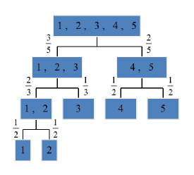
Figure 1: Two-party strong five-sided DR protocol saturating Kitaev’s bound. The digits inside the boxes denote the possible outcomes. Each branching represents a strong imbalanced coin flip. The fractions beside each branch give the probability for the outcomes within the box below conditional on the outcomes in the box above. Thus, for the leftmost branch we have that the probability for the outcome equals $1/2\cdot 2/3\cdot 3/5=1/5$, etc.

III.3 A family of optimal multi-party strong dice rolling protocols

The above construction readily allows for the introduction of a family of $2m$-party strong $n^{m}$-sided DR protocols saturating the generalization of Kitaev’s bound, eq. (18). The idea is to sequentially have distinct pairs of parties strongly roll a dice to eliminate some of the outcomes, until a single outcome is obtained. Thus, in the case of four parties and nine outcomes, in the first stage the first and second parties strongly roll a three-sided dice. If its outcome is $1$, outcomes $4$ to $9$ are eliminated, while if its outcome is $2$, outcomes $1$ to $3$ and $7$ to $9$ are eliminated, etc. Suppose, for example, that outcomes $1$ to $6$ are eliminated. Then in the second stage parties three and four strongly roll a three-sided dice, where if its outcome is $1$, then the final outcome of the protocol is $7$, while if its outcome is $2$, then the final outcome is $8$, etc. In general, for $2m$-parties and an $n^{m}$-sided dice, the protocol consists of $n$ stages. In each stage a different pair of parties strongly rolls an $n$-sided dice. As there are a total of 2$m$ parties, each party strongly participates in a dice roll once. In order to force the outcome they desire, the $2m-1$ dishonest parties must bias the result of the dice roll in which the honest party participates, and since at any stage there is only a single outcome that can lead to the desired outcome, the dishonest parties can maximally bias the outcome with a probability of $\left(1/n\right)^{1/2}+\bar{\epsilon}$, which saturates the generalization of Kitaev’s bound, eq. (18).

It is not straightforward to generalize this scheme to any number of parties and outcomes. The problem is that we have introduced an ordering, which dependent on it, may in general render the protocol asymmetric in the biases, or even trivial by allowing the dishonest parties to force the outcome that they desire. This can be fixed by making use of optimal weak DR to decide the ordering. Unfortunately, this comes at the expense of optimality, i.e. eq. (18) is no longer saturated. Nevertheless, protocols incorporating optimal weak and strong DR protocols may give rise to biases remarkably close to the inherent bounds. As an example, consider the following three-party strong three-sided DR protocol. In the first round Alice, Bob and Clare weakly roll a three-sided dice. The winner then randomly selects a number $a\in\left\{1,\,3\right\}$ and informs the two losers of his/her choice. The two losers then strongly flip a coin. Denote its outcome by $b\in\left\{0,\,1\right\}$. The outcome of the protocol is $\left(a+b\right)\,\mathrm{mod}\,3$. It is easy to verify that the maximal probability of any two parties to successfully bias to any of the outcomes approximately equals $0.69363$, while from eq. (19) $q=\left(1/3\right)^{1/3}\simeq 0.69336$. That is, a difference of $0.027\,\%$. Similarly, to the optimal $2m$-party $n^{m}$-sided DR protocols described above, this protocol can be generalized to a family of $3n$-party $3^{n}$-sided DR protocol, with each giving rise to the same bias.

To complete the discussion we should mention that strong DR is nontrivial also in classical settings. Indeed, the classical biases for two-party $N$-sided DR are constrained by the following set of inequalities Kitaev

$$\left(1-\left.\bar{P}_{A}^{\left(i\right)}\right.^{*}\right)\left(1-\left.\bar{P}_{B}^{\left(j\right)}\right.^{*}\right)\leq\frac{N-2}{N}+\frac{1}{N}\delta_{i,\,j}\,,\qquad i,\,j\in\left\{1,\,\dots,\,N\right\}\,.$$ (37)

It is straightforward to verify that these inequalities are “weaker” than the corresponding Kitaev bound, and hence allow for higher biases.

III.4 A family of three-round two-party strong dice rolling protocols

In this subsection we introduce a family of three-round strong DR protocols, which generalizes Colbeck’s entanglement-based strong CF protocol Colbeck to any number of outcomes. Suppose Alice and Bob want to strongly roll an $N$-sided dice using a minimal number of rounds of communication. Then they may proceed as follows. Alice prepares a pair of systems in the state $\left|\psi_{N}\right\rangle\otimes\left|\psi_{N}\right\rangle$, where $\left|\psi_{N}\right\rangle=\frac{1}{\sqrt{N}}\sum_{i=1}^{N}\left|i\right\rangle\otimes\left|i\right\rangle$, and sends the second half of each system to Bob. Bob randomly selects one of the systems to serve as the dice and informs Alice of his selection. Alice and Bob then measure their half of the selected system in the Schmidt basis. The outcome of this measurement is the outcome of the dice roll. Finally, Alice sends Bob her half of system that was not selected, and he verifies it was indeed prepared in the state $\left|\psi_{N}\right\rangle$.

Following a similar argument to Colbeck’s, Alice’s and Bob’s maximal probabilities of biasing to any of the outcomes are given by

$$\left.P_{A}^{\left(i\right)}\right.^{*}=\frac{N+1}{2N}\,,\qquad\left.P_{B}^{\left(i\right)}\right.^{*}=\frac{2N-1}{N^{2}}\,,\qquad\left\{i=1,\,\dots,\,N\right\}$$ (38)

Thus, for $N=3$ $\epsilon_{A}^{\left(i\right)}=\left.P_{A}^{\left(i\right)}\right.^{*}-1/3=1/3$ and $\epsilon_{B}^{\left(i\right)}=\left.P_{B}^{\left(i\right)}\right.^{*}-1/3=2/9$. Interestingly, in the limit where $N\rightarrow\infty$, $\left.P_{A}^{\left(i\right)}\right.^{*}\rightarrow 1/2$ , $\left.P_{B}^{\left(i\right)}\right.^{*}\rightarrow 2/N$, so that $\left.P_{A}^{\left(i\right)}\right.^{*}\cdot\left.P_{B}^{\left(i\right)}\right.^{*}\rightarrow 1/N$. Hence, in this limit Kitaev’s bound is nontrivially saturated in a finite number of rounds, albeit at a cost of a high asymmetry of the biases.

IV Conclusions

We have defined a novel mutli-outcome generalization of quantum CF, which we have termed quantum DR. We have analyzed both its weak and strong variants. Specifically, we proved by construction that in quantum settings (i) weak $N$-sided dice rolling – the problem of $N$ remote distrustful parties having to decide on a number between $1$ and $N$ with party $i$ preferring the $i$-th outcome – admits an arbitrarily small bias for any value of $N$, and (ii) two-party strong $N$-sided dice rolling – the problem of two remote distrustful parties having to decide on a number between $1$ and $N$ without any party being aware of the other’s preference – saturates the corresponding generalization of Kitaev’s bound for any value of $N$. In addition, we also made use of this last result to introduce a family of optimal $2m$-party strong $n^{m}$-sided DR protocols for any value of $m$ and $n$. The question of whether this is also possible in the general case of any number of parties and outcomes remains open for now.

Appendix A

For any weak DR protocol, based on weak imbalanced CF according to the scheme presented in section II, party $n$’s maximum chance of losing is given by

$$\bar{P}_{n}^{*} = \frac{N-1}{N}+\bar{\epsilon}_{n}$$

$$= \mbox{$\bar{\Pi}$}_{n-1}^{*}+\sum_{k=n}^{N-1}\mbox{$\bar{\Pi}$}_{k}^{*}\prod_{j=0}^{k-n}\left(1-\bar{\Pi}_{n-1+j}^{*}\right)$$

$$= \frac{n-1}{n}+\bar{\delta}_{n-1}+\sum_{k=n}^{N-1}\left(\frac{1}{k}+\bar{\delta}_{k}\right)\left(\frac{1}{n}-\bar{\delta}_{n-1}\right)\prod_{j=1}^{k-n-1}\left(\frac{n+j}{n+j+1}-\bar{\delta}_{n-1+j}\right)\,,$$

where $\bar{\Pi}_{k}^{*}$ is party $n$’s maximum chance of losing stage $k$ conditional on having made it to that round and $\bar{\delta}_{k}$ the corresponding bias. If we now let $\bar{\delta}_{\mathrm{max}}^{\left(n\right)}\hat{=}\max_{k}\bar{\delta}_{k}$ and $\bar{\delta}_{\mathrm{min}}^{\left(n\right)}\hat{=}\min_{k}\bar{\delta}_{k}$ ($k=n-1,\,\dots,\,N-1$), then

$$\bar{\epsilon}_{n} \leq \bar{\delta}_{\mathrm{max}}^{\left(n\right)}+\bar{\delta}_{+}^{\left(n\right)}\sum_{k=n}^{N-1}\left(\frac{1}{n}-\bar{\delta}_{\mathrm{min}}^{\left(n\right)}\right)\prod_{j=1}^{k-n-1}\left(\frac{n+j}{n+j+1}-\bar{\delta}_{\mathrm{min}}^{\left(n\right)}\right)-\bar{\delta}_{\mathrm{min}}^{\left(n\right)}\sum_{k=n}^{N-1}\left(\frac{1}{k}+\bar{\delta}_{\mathrm{max}}^{\left(n\right)}\right)\prod_{j=1}^{k-n-1}\left(\frac{n+j}{n+j+1}-\bar{\delta}_{\mathrm{min}}^{\left(n\right)}\right)$$

$$-\bar{\delta}_{\mathrm{min}}^{\left(n\right)}\sum_{k=n}^{N-1}\left(\frac{1}{k}+\bar{\delta}_{\mathrm{max}}^{\left(n\right)}\right)\left(\frac{1}{n}-\bar{\delta}_{\mathrm{min}}^{\left(n\right)}\right)\sum_{m=1}^{k-n-1}\prod_{j\neq m}\left(\frac{n+j}{n+j+1}-\bar{\delta}_{\mathrm{min}}^{\left(n\right)}\right)$$

$$< \bar{\delta}_{\mathrm{max}}^{\left(n\right)}+\bar{\delta}_{\mathrm{max}}^{\left(n\right)}\sum_{k=n}^{N-1}\frac{1}{n}\prod_{j=1}^{k-n-1}\frac{n+j}{n+j+1}$$

$$< N\bar{\delta}_{\mathrm{max}}^{\left(n\right)}$$

Hence, if each of the weak imbalanced CF protocols, used to implement the DR protocol, are such that $\bar{\delta}_{\mathrm{max}}^{\left(n\right)}\ll 1/N$ for any $n$, an honest party’s winning probability tends to $1/N$.

Appendix B

Alice’s maximal bias

Most generally Alice can prepare any state of the form

$$\left|\psi_{0}^{\prime}\right\rangle=\sum_{i,\,j=\uparrow,\,\downarrow}\alpha_{ij}\left|ij\right\rangle\otimes\left|\Phi_{ij}\right\rangle\,,$$ (41)

where the $\left|\Phi_{ij}\right\rangle$ are states of some ancillary system at her possession. After Bob applies $U_{\eta}$ the resulting composite state is given by

$$\left|\psi_{1}^{\prime}\right\rangle = U_{\eta}\left|\psi_{0}^{\prime}\right\rangle\otimes\left|\downarrow\right\rangle$$

$$= \alpha_{\uparrow\uparrow}\left(\sqrt{\frac{p}{p+\eta}}\left|\uparrow\uparrow\downarrow\right\rangle+\sqrt{\frac{\eta}{p+\eta}}\left|\uparrow\downarrow\uparrow\right\rangle\right)\otimes\left|\Phi_{\uparrow\uparrow}\right\rangle+\alpha_{\uparrow\downarrow}\left|\uparrow\downarrow\downarrow\right\rangle\otimes\left|\Phi_{\uparrow\downarrow}\right\rangle$$

$$+\alpha_{\downarrow\uparrow}\left(\sqrt{\frac{p}{p+\eta}}\left|\downarrow\uparrow\downarrow\right\rangle+\sqrt{\frac{\eta}{p+\eta}}\left|\downarrow\downarrow\uparrow\right\rangle\right)\otimes\left|\Phi_{\downarrow\uparrow}\right\rangle+\alpha_{\downarrow\downarrow}\left|\downarrow\downarrow\downarrow\right\rangle\otimes\left|\Phi_{\downarrow\downarrow}\right\rangle\,.$$

The probability that Bob does not find find the second and third qubits in the state $\left|\uparrow_{2}\downarrow_{3}\right\rangle$ is

$$\bar{P}_{\uparrow\downarrow}=1-P_{\uparrow\downarrow}=1-\frac{\left|\alpha_{\uparrow\uparrow}\right|^{2}p+\left|\alpha_{\downarrow\uparrow}\right|^{2}p}{p+\eta}\,,$$ (43)

and the resulting composite state then is

$$\left|\psi_{2}^{\prime}\right\rangle = \mathcal{N}\left(\alpha_{\uparrow\uparrow}\sqrt{\frac{\eta}{p+\eta}}\left|\uparrow\downarrow\uparrow\right\rangle\otimes\left|\Phi_{\uparrow\uparrow}\right\rangle+\alpha_{\uparrow\downarrow}\left|\uparrow\downarrow\downarrow\right\rangle\otimes\left|\Phi_{\uparrow\downarrow}\right\rangle\right.$$ (44)

$$\left.+\alpha_{\downarrow\uparrow}\sqrt{\frac{\eta}{p+\eta}}\left|\downarrow\downarrow\uparrow\right\rangle\otimes\left|\Phi_{\downarrow\uparrow}\right\rangle+\alpha_{\downarrow\downarrow}\left|\downarrow\downarrow\downarrow\right\rangle\otimes\left|\Phi_{\downarrow\downarrow}\right\rangle\right)\,,$$

where $\mathcal{N}$, the normalization, is

$$\frac{1}{\mathcal{N}^{2}}=1-\frac{p}{p+\eta}\left(\left|\alpha_{\uparrow\uparrow}\right|^{2}+\left|\alpha_{\downarrow\uparrow}\right|^{2}\right)\,.$$ (45)

The probability that Alice passes the test is therefore given by

$$P_{\mathrm{test}}=\left\|\left\langle\xi\mid\psi_{2}^{\prime}\right\rangle\right\|^{2}=\mathcal{N}^{2}\left\|\alpha_{\uparrow\downarrow}\sqrt{\frac{1-p-\eta}{1-p}}\left|\Phi_{\uparrow\downarrow}\right\rangle+\alpha_{\downarrow\uparrow}\sqrt{\frac{\eta^{2}}{\left(1-p\right)\left(p+\eta\right)}}\left|\Phi_{\downarrow\uparrow}\right\rangle\right\|^{2}\,.$$ (46)

The maximum obtains for $\left|\Phi_{\uparrow\downarrow}\right\rangle=\left|\Phi_{\downarrow\uparrow}\right\rangle$. This choice of the ancillary states does not affect the maximum of $\bar{P}_{\uparrow\downarrow}$. Hence, Alice obtains no advantage by using ancillary systems and we can do away with them. Alice’s maximum cheating probability is then

$$P_{A}^{*}=\max_{\alpha_{ij}}\bar{P}_{\uparrow\downarrow}\cdot P_{\mathrm{test}}\,,$$ (47)

where now

$$\bar{P}_{\uparrow\downarrow}\cdot P_{\mathrm{test}}=\left|\alpha_{\uparrow\downarrow}\sqrt{\frac{1-p-\eta}{1-p}}+\alpha_{\downarrow\uparrow}\sqrt{\frac{\eta^{2}}{\left(1-p\right)\left(p+\eta\right)}}\right|^{2}$$ (48)

($\bar{P}_{\uparrow\downarrow}=1/\mathcal{N}^{2}$). Clearly, this expression is maximum when $\alpha_{\uparrow\uparrow}=\alpha_{\downarrow\downarrow}=0$. Therefore, to maximize her chance of successfully cheating Alice will prepare a state of the form

$$\left|\psi_{0}^{\prime}\right\rangle=\sqrt{1-\delta}\left|\uparrow_{1}\downarrow_{2}\right\rangle+\sqrt{\delta}\left|\downarrow_{1}\uparrow_{2}\right\rangle\,,$$ (49)

where with no loss of generality we have set $\alpha_{\uparrow\downarrow}=\sqrt{1-\delta}$ and $\alpha_{\downarrow\uparrow}=\sqrt{\delta}$. So that

$$P_{A}^{*}=\max_{\delta}\left(\sqrt{\frac{\left(1-p-\eta\right)\left(1-\delta\right)}{1-p}}+\sqrt{\frac{\eta^{2}\delta}{\left(1-p\right)\left(p+\eta\right)}}\right)^{2}\,.$$ (50)

Bob’s maximal bias

Bob wins and passes the test whenever Alice does not find the first qubit in the state $\left|\uparrow\right\rangle$. The probability for this is just $p+\eta$. This gives an upper bound on Bob’s maximal cheating probability, which is reached if Bob always announces that he has won. That is,

$$P_{B}^{*}=p+\eta\,.$$ (51)

References

- (1) M. Blum, in Advances in Cryptology: A Report on CRYPTO 81 (1982).
- (2) J. Kilian, in Proceedings of the 20th Annual ACM Symposium on the Theory of Computing (1988).
- (3) C.H. Bennett and G. Brassard, in Proceedings of the 1984 IEEE International Conference on Computers, Systems and Signal Processing (1984).
- (4) L. Goldenberg, L. Vaidman and S. Wiesner, Phys. Rev. Lett. 82, 3356 (1999).
- (5) Prior to Mochon’s work Mochon , there were serious doubts as to the possibility of WCF with arbitrarily small bias. Quantum gambling was introduced as an example of a quantum cryptographic task, impossible in classical settings, which is nevertheless unconditionally secure in the sense that it does away with the notion of cheating; both the casino and the player do not have to follow any “honest” protocol, but rather are allowed to do anything to maximize their gain.
- (6) D. Aharonov, A. Ta-Shma, U. Vazirani and A.C. Yao, in Proceedings of the 32nd Annual ACM Symposium on the Theory of Computing (2000).
- (7) R.W. Spekkens and T. Rudolph, Quantum Inform. Compu. 2, 66 (2002).
- (8) R.W. Spekkens and T. Rudolph, Phys. Rev. A 65, 012310 (2001).
- (9) A. Ambainis, in Proceedings of the 33rd Annual ACM Symposium on the Theory of Computing (2001).
- (10) A. Kitaev, unpublished. The proof of Kitaev’s bound is recreated in Multi-party .
- (11) R.W. Spekkens and T. Rudolph, Phys. Rev. Lett. 89, 227901 (2002).
- (12) C. Mochon, in 45th Symposium on Foundations of Computer Science (2004).
- (13) C. Mochon, Phys. Rev. A 72, 022341 (2005).
- (14) C. Mochon, arXiv:0711.4114 [quant-ph].
- (15) A. Chailloux and I. Kerenidis, arXiv:0904.1511 [quant-ph].
- (16) A. Ambainis, H. Buhrman, Y. Dodis and H. Rohrig, in Proceedings of the 19th IEEE Annual Conference on Computational Complexity (2004).
- (17) See, for example, the proof in C. Döscher and M. Keyl, Fluct. Noise Lett. 4, R125 (2002). Even though this proof formally covers only the balanced case, its reasoning is also applicable to the imbalanced case.
- (18) R. Colbeck, Phys. Lett. A 362, 390 (2007).