Muon-Spin Spectroscopy of the organometallic spin $1/2$ kagomé-lattice compound Cu(1,3-benzenedicarboxylate)

Abstract

Using muon spin resonance we examine the organometallic hybrid compound Cu(1,3-benzenedicarboxylate) [Cu(1,3-bdc)], which has structurally perfect spin 1/2 copper kagomé planes separated by pure organic linkers. This compound has antiferromagnetic interactions with Curie-Weiss temperature of $-33$ K. We found slowing down of spin fluctuations starting at $T=1.8$ K, and that the state at $T\rightarrow 0$ is quasi-static with no long-range order and extremely slow spin fluctuations at a rate of $3.6$ $\mu$sec^-1. This indicates that Cu(1,3-bdc) behaves as expected from a kagomé magnet and could serve as a model kagomé compound.

Date text]date

The experimental search for an ideal two dimensional, spin 1/2, kagomé compound, which has no out-of-plane interactions and no impurities on the kagomé plane, has powered tremendous experimental effort in recent years Samples . Yet, all compounds studied today have shortcomings. Recently, a promising copper-based metal organic hybrid compound Cu(1,3-bdc) was synthesized by Nytko et al. Emiliy . This compound has an ideal kagomé lattice structure as indicated by X-ray, the spins are naturally 1/2, and there are no Zn ions or any other candidates to substitute the Cu on the kagomé plane. The goal of this paper is to show that from a magnetic point of view Cu(1,3-bdc) shows the signatures of the high degree of frustration expected on the kagomé lattice. This is done by demonstrating that the inter-plane interactions are small enough compared to the intra-plane interactions that no long range order is found at temperatures well below the interaction energy scale, and by characterizing the ground state properties. The experimental tool is muon spin resonance ($\mu$SR). Our major finding is that the state at the lowest temperature investigated is quasi-static with extremely slow spin fluctuations. This type of behavior is similar to a huge class of frustrated magnets KagomeNoDeep ; Canonical . Therefore, Cu(1,3-bdc) could serve as a model spin 1/2 kagomé compound.

Cu(1,3-bdc) is shorthand for Cu(1,3-benzenedicarboxylate). The kagomé planes are separated by organic linkers, each linker being a benzene molecule with two corners featuring a carboxylate ion instead of the standard H ion. If one were to label the corners 1-6 consecutively, the two corners with the carboxylate ions would be the 1st and 3rd. The Cu ions located on the kagomé plane are linked by O-C-O ions, while inter-plane Cu ions are linked by O-5C-O ions. The basic elements of Cu(1,3-bdc) are depicted in Fig. 1. Magnetization measurements found antiferromagnetic Curie-Weiss temperature of -33 K Emiliy . Strong antiferromagnetic exchange between Cu²⁺ ions linked by a carboxylate molecule was also found in the trinuclear compound Cu₃(O₂C₁₆H₂₃)·1.2C₆H₁₂ StonePRB07 . Heat capacity shows a peak at $T\simeq 2$ K Emiliy .

The powder we examined contains Cu(1,3-bdc) in the form of blue crystalline plates. However, it is mixed with some green plates of copper-containing ligand oxidation by-product C₃₂H₂₄Cu₆O₂₆, which cannot be separated from the blue plates. To the naked eye it looks as if about 10% of the plates are green. However, as we demonstrate below, the $\mu$SR signal from Cu(1,3-bdc) can be separated from the C₃₂H₂₄Cu₆O₂₆ signal. Our sample was pressed into a Cu holder for good thermal contact.

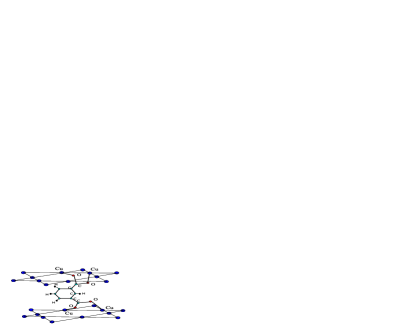
Figure 1: (Color online) The Cu(1,3-bdc) structure showing the kagomé planes and the inter-plane and intra-plane superexchange path.

Muon spin rotation and relaxation ($\mu$SR) measurements were performed at the Paul Scherrer Institute, Switzerland (PSI) in the low temperature facility spectrometer with a dilution refrigerator. The measurements were carried out with the muon spin tilted at $45^{\circ}$ relative to the beam direction. Positrons emitted from the muon decay were collected simultaneously in the forward-backward (longitudinal) and the up-down (transverse) detectors with respect to the beam direction. Transverse field (TF) measurements, where the field is perpendicular to the muon spin direction, were taken at temperatures ranging from 0.9 K to 6.0 K with a constant applied field of $H=1$ kOe. Zero-field (ZF) measurements were taken in the longitudinal configuration at a temperature ranging from 0.9 K to 2.8 K. The longitudinal-field (LF) measurements, where the field is parallel to the muon spin direction, were taken at several different fields between 50 Oe and 3.2 kOe with a constant temperature of 0.9 K. We also performed a field calibration measurement using a blank silver plate providing the muon rotation frequency $f_{s}=13.67$ MHz at the applied TF of 1 kOe.

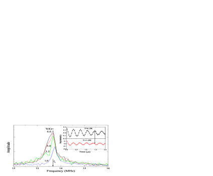
Figure 2: (Color online) FFT of the asymmetry data in a field of 1 kOe transverse to the initial muon spin dirrection. $f_{s}$  is the reference fequency in pure silver. Inset: transverse field asymmetry in the time domain and a rotating reference frame.

In the inset of Fig. 2 we depict by symbols the muon decay asymmetry in a reference frame rotated at $H=200$ Oe less than the TF. In the main panel of Fig. 2 we show the fast Fourier transform (FFT) of the TF data at some selected temperatures. The FFT of the highest temperature, 6 K, shows a wide asymmetric peak with extra weight towards low frequencies. At 3 K the wide asymmetric peak separates into two different peaks shifting in opposite directions. At even lower temperatures the low frequency peak vanishes. We assign the latter peak to muons that stop in Cu(1,3-bdc) since such a wipe-out of the signal is typical of slowing down of spin fluctuations, which in Cu(1,3-bdc) is expected near $2$ K.

Despite the disappearance of the second peak in the frequency domain, its contribution in the time domain is clear. The high frequency peak in the main panel of Fig. 2 corresponds to the signal surviving for a long time in both insets of Fig. 2. The broad and disappearing peak in the main panel corresponds to the fast decaying signal in the first 0.2 $\mu$sec seen in the lower inset. The arrow in the inset demonstrates the frequency shift. Consequently we fit the function

$$A_{TF}(t)=A_{1}e^{-(R_{1}t)^{2}/2}cos(\omega_{1}t+\varphi)+A_{2}e^{-R_{2}t}cos(\omega_{2}t+\varphi)+B_{g}$$ (1)

to our data in the time domain globally, where the parameters $R_{1}$ and $\omega_{1}$ are the relaxation and angular frequency of the by-product, and $R_{2}$ and $\omega_{2}$ are the relaxation and angular frequency of the kagomé part. The parameters $A_{1}=0.049(4),$ $A_{2}=0.125(3),$ $R_{1}=0.13(1)$ ($\mu\sec^{-1}$), $\varphi$ and $B_{g}$ are shared in the fit, while $R_{2},\omega_{1},\omega_{2}$ are free. The quality of the fit is represented in the inset of Fig. 2 by the solid lines. The ratio of $A_{1}$ to $A_{2}$ supports the assignment of the fast relaxing signal to Cu(1,3-bdc).

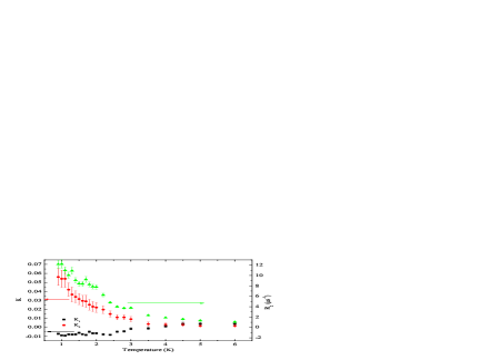
Figure 3: (Color online) The muon shift from C₃₂H₂₄Cu₆O₂₆ $K_{1}$ and from Cu(1,3-bdc) $K_{2}$, and the relaxation rate from Cu(1,3-bdc) $R_{2}$ versus temperature.

In Fig. 3 we plot the shift, $K_{1,2}=(\omega_{s}-\omega_{1,2})/\omega_{s}$, versus temperature, where $\omega_{s}=2\pi f_{s}$. As expected $K_{2}$ increases with decreasing temperatures. The small decrease of $K_{1}$ is not expected and is not clear to us at the moment. The muon transverse relaxation, $R_{2}$, is also presented in Fig. 3. It has roughly the same temperature behavior as the shift, $K_{2}$. However, at $T=$1.8 K $R_{2}$ seems to flatten out before increasing again around 1 K. This is somewhat surprising.

The field at the muon site is given by $\mathbf{B}=\mathbf{H}-\sum_{k}\tilde{A}_{k}\left\langle\mathbf{S}_{k}\right\rangle$ where $\left\langle\mathbf{S}_{k}\right\rangle$ is the thermal average of the spins neighboring the muon, and $\tilde{A}_{k}$ is the hyperfine interaction with each neighboring spin. Assuming a distribution of hyperfine fields in the $\hat{z}$ direction one can write $\tilde{A}_{k}$ as a sum of a mean value $\overline{A_{k}}$ plus a fluctuating component $\delta A_{k}$. For the distribution

$$\rho\left(\delta A_{k}\right)=\frac{1}{\pi}\frac{\sigma_{k}}{\left(\delta A_{k}\right)^{2}+\sigma_{k}^{2}}$$ (2)

one finds that the shift is given by $K_{2}=\left\langle\mathbf{S}_{k}\right\rangle\sum_{k}\overline{A_{k}}/H$ and $R_{2}=\gamma_{\mu}\left\langle\mathbf{S}_{k}\right\rangle\sum_{k}\sigma_{k}$ CarrettaHFM . To test this derivation it is customary to plot the macroscopic magnetization $M$ measured with a SQUID magnetometer versus $K_{2}$. This is depicted in Fig. 4(a). The magnetization is also measured at $1$ kOe. The plot indicates that in the temperature range where both $M$ and $K_{2}$ are available they are proportional to each other. Therefore, $\sum_{k}\overline{A_{k}}$ is temperature-independent.

If the $\sigma_{k}$ are also temperature-independent parameters we expect $R_{2}\propto K_{2}$. A plot of $R_{2}$ versus $K_{2}$, shown in Fig. 4(b), indicates that $R_{2}$ is not proportional to or even does not depend linearly on $K_{2}$ and a kink is observed at $T_{0}=1.8$ K. This result suggests a change in the hyperfine fields distribution at $T_{0}$. An interesting possible explanation for such a change is a response of the lattice to the magnetic interactions via a magnetoelastic coupling KerenPRL01 . However, unlike a similar situation in a pyrochlore lattice SagiPRL05 , it seems that here the lattice is becoming more ordered upon cooling since the rate of growth of $R_{2}$ below $T_{0}$ is lower than at higher temperatures.

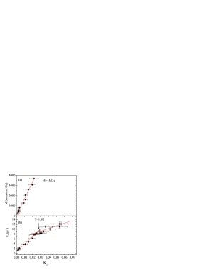
Figure 4: (Color online) (a) Magnetization versus the muon shift in Cu(1,3-bdc). (b) The muon relaxation rate versus the muon shift in Cu(1,3-bdc).

The $\mu$SR LF data including ZF are presented in Fig. 5. The LF data at the lowest temperature of $0.9$ K are depicted in panel (a). At this temperature and a field of 50 Oe, the muon asymmetry shows a minimum at around 0.1 $\mu$sec. At longer times the asymmetry recovers. The origin of this dip is the presence of a typical field scale around which the muon spin nearly completes an oscillation. However, the field distribution is so wide that the oscillation is damped quickly. The origin of the recovery is the fact that some of the muons experience nearly static field in their initial field direction during the entire measured time. These muons do not lose their polarization while others do. When the external field increases, the dip moves to earlier times (as the field scale increases) and the asymptotic value of the asymmetry increases as well (as more muons do not relax).

The ZF data at three different temperature are shown in Fig. 5(b). As the temperature decreases the relaxation rate increases due to the slowing down of spin fluctuations, until at the lowest temperature the dip appears. We saw no difference in the raw data between 1.0 and 0.9 K and therefore did not cool any further.

These are unusual $\mu$SR data in a kagomé magnet, in the sense that the spin fluctuations are slow enough compared to the internal field scale to expose the static nature of the muon spin relaxation function, namely, the dip, and to allow calibration of the internal field distribution. Other kagomé magnets show the same general behavior but without this dip KagomeNoDeep . The data indicate the absence of long-range order and the presence of quasi-static field fluctuation. If the ground state had long-range order, the muon would have oscillated several times due to the internal magnetic field. Similarly, if the ground state was dynamic we would not have seen a recovery of the muon polarization after a long time.

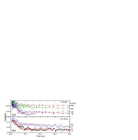
Figure 5: (Color online) The asymmetry at various longitudinal fields and T=0.9 K (a). The asymmetry at zero field and various temperatures (b)

To analyze this type of muon spin relaxation function, a theoretical polarization function $P(\nu,\Delta,H,t)$ must be generated. It depends on the random field distribution $\rho(\mathbf{B})$, the spin fluctuations rate $\nu$ defined by $\left\langle\mathbf{B}(t)\mathbf{B}(0)\right\rangle=\left\langle B^{2}\right\rangle e^{-2\nu t}$ , where $B$ is the internal local field, and the LF $H$. In ZF or small LF field, standard perturbation methods for calculating relaxation functions do not apply and a special method for calculating $P$ is required. This function is produced in two steps. In the first step the static muon polarization is generated using the double projection expression

$$\overline{P}_{z}(0,\Delta,H,t)=\int\rho(\mathbf{B})\left[\frac{B_{z}^{2}}{\mathbf{B}^{2}}+\frac{B_{x}^{2}+B_{y}^{2}}{\mathbf{B}^{2}}\cos(\gamma_{\mu}\left|\mathbf{B}\right|t)\right]d^{3}\mathbf{B.}$$ (3)

We found that the Gaussian field distribution

$$\rho(\mathbf{B})=\frac{\gamma_{\mu}^{3}}{(2\pi)^{3/2}\Delta^{3}}\exp\left(-\frac{\gamma_{\mu}^{2}[\mathbf{B-}H\mathbf{\hat{z}}]^{2}}{2\Delta^{2}}\right)$$ (4)

works best. This $\overline{P}_{z}(0,\Delta,H,t)$ is known as the Static Gaussian Kubo-Toyabe LF relaxation function Hayano .

In the second step the dynamic fluctuations are introduced. One method of doing so is using the Voltera equation of the second kind Keren

$$\overline{P}_{z}(\nu,H,\Delta,t) =e^{-\nu t}\overline{P}_{z}(0,H,\Delta,t)+$$

$$\nu\int_{0}^{t}dt^{\prime}\overline{P}_{z}(\nu,H,\Delta,t-t^{\prime})e^{-\nu t^{\prime}}\overline{P}_{z}(0,H,\Delta,t^{\prime}).$$ (5)

The function $\overline{P}_{z}(0,H,\Delta,t^{\prime})$ is taken from the first step. The factor $e^{-\nu t}$ is the probability to have no field changes up to time $t$. The factor $e^{-\nu t^{\prime}}\nu dt^{\prime}$ is the probability density to experience a field change only between $t^{\prime}$ and $t^{\prime}+dt^{\prime}$. The first term on the r.h.s is the polarization at time $t$ due to muons that did not experience any field changes. The second term on the r.h.s is the contribution from those muons that experienced their first field change at time $t^{\prime}$. The factor $e^{-\nu t^{\prime}}\overline{P}_{z}(0,H,\Delta,t^{\prime})\nu dt^{\prime}$ is the amplitude for the polarization function evolving from time $t^{\prime}$ to $t$, which can include more field changes recursively. This equation can be solved numerically NumericalRecipes and $\overline{P}_{z}(\nu,H,\Delta,t)$ is known as the Dynamic Gaussian Kubo-Toyabe LF relaxation function Hayano .

The experimental asymmetry is fitted with $A_{LF}=A_{0}\overline{P}_{z}(\nu,H,\Delta,t)+B_{g}$. The relaxation from the second green phase is very small and is absorbed in the background factor $B_{g}$. In the fit of the field-dependence experiment at the lowest temperature, presented in Fig. 5(a) by the solid lines, $\Delta,\nu,A_{0}$ and $B_{g}$ are shared parameters. We found $\Delta=19.8(4)$ MHz and $\nu=3.6(2)$ $\mu\sec^{-1}$. This indicates that the spins are not completely frozen even at the lowest temperature.

When analyzing the ZF data at a variety of temperatures, shown in Fig. 5(b) by the solid lines, we permit only $\nu$ to vary. The fit is good at the low temperatures but does not capture the 2.8 K data at early times accurately. However, the discrepancy is not big enough to justify adding more fit parameters. We plot the temperature dependence of the fluctuation rate in Fig. 6. $\nu$ hardly changes while the temperature decreases from $T=2.8~{}$K down to $T_{0}=1.8~{}$K. From $T_{0}$, $\nu$ decreases with decreasing temperatures, but saturates below $1$ K. This type of behavior was observed in a variety of frustrated kagomé (Ref.  KagomeNoDeep ) and pyrochlore (Ref. Canonical ) lattices. It is somewhat different from classical numerical simulations where $\nu$ decreases with no saturation kerenPRL94 ; RobertPRL08 . In fact, the numerical $\nu$ is a linear function of the temperature over three orders of magnitude in $T$ RobertPRL08 .

The inset of Fig. 6 shows $\nu$ as a function of temperature near $T_{0}$ on a log-log scale where slowing down begins. Only near $T_{0}$ are our data consistent with a linear relation

$$\nu-\nu_{\infty}=\nu_{0}(T-T_{0}),$$

where $\nu_{\infty}$ is the high temperature fluctuation rate. The discrepancy with the numerical work might be because $\mu$SR probes field correlations involving several spins nearing the muon, while the simulations concentrate on spin-spin auto correlations (with a decay $\Gamma_{a}$ compared here with $\nu$). At our lowest temperature the rotations of ensemble of spins are already coherent therefore field and spin correlations are not identical. Another possibility is that the saturation of $\nu$ with decreasing $T$ is a pure quantum effect not captured by the classical simulations.

Figure 6: (Color online) The fluctuation rate $\nu$ versus temperature. Inset; $\nu$ near $1.8$ K on a log-log scale. The error bars are smaller than the symbol size.

To summarize, we found that Cu(1,3-bdc) has a special temperature $T_{0}=1.8$ K. Upon cooling, the susceptibility, as measured by the $\mu$SR, grows monotonically even past this temperature. The muon spin line-width also grows but halts around this temperature. This might be explained by a subtle structural transition, but low temperature structural data are required. At $T_{0}$ the slowing down of spin fluctuations begins, but the spins remain dynamic with no long range order. The rate of the spin fluctuations appears to be linear near $T_{0}$, but becomes saturated at the lowest T. This general behavior is similar to other kagomé compounds, though new features are seen here. Therefore, considering its lattice, Cu(1,3-bdc) could serve as a model compound for spin $1/2$ kagomé magnet.

We acknowledge financial support from the Israel U.S.A. Binational Science Foundation, the European Science Foundation (ESF) for the ‘Highly Frustrated Magnetism’ activity, and the European Commission under the 6th Framework Program through the Key Action: Strengthening the European Research Area, Research Infrastructures. Contract n^∘: RII3-CT-2004-506008.

References

- (1) A. P. Ramirez, Annu. Rev. Mater. Sci. 24, 453 (1994); Z. Hiroi et al., J. Phys. Soc. Jpn. 70, 3377 (2001); I. S. Hagemann, Q. Huang, X. P. A. Gao, A. P. Ramirez, and R. J. Cava, Phys. Rev. Lett. 86, 894 (2001); M. P. Shores, E. A. Nytko, B. M. Bartlett, and D. G. Nocera, J. Am. Chem. Soc. 127, 13 462 (2005); P. Bordet, I. Gerlard, K. Marty, A. Ibanez, J. Robert, V. Simonet, B. Canals, R. Ballou and P.Lejay Journal of Physics: Condensed Matter 18 5147-5153 (2006). J. S. Helton, K. Matan, M. P. Shores, E. A. Nytko, B. M. Barlett, Y. Yoshida, Y. Takano, A. Suslov, Y. Qiu, J. H. Chung, D. G. Nocera, and Y. S. Lee, Phys. Rev. Lett. 98, 107204 (2007).
- (2) Emily A. Nytko, Joel S. Helton, Peter Müller, and Daniel G. Nocera, J. Am. Chem. Soc. 130, 2922 (2008).
- (3) A. Keren, Y. J. Uemura, G. Luke, P. Mendels, M. Mekata, and T. Asano, Phys. Rev. Lett. 84, 3450 (2000); A. Fukaya, Y. Fudamoto, I. M. Gat, T. Ito, M. I. Larkin, A. T. Savici, Y. J. Uemura, P. P. Kyriakou, G. M. Luke, M. T. Rovers, K. M. Kojima, A. Keren, M. Hanawa, and Z. Hiroi, Phys. Rev. Lett. 91, 207603 (2003); D. Bono, P. Mendels, G. Collin, N. Blanchard, F. Bert, A. Amato, C. Baines, and A. D. Hillier, Phys. Rev. Lett. 93, 187201 (2004).
- (4) S. R. Dunsiger et al., Phys. Rev. B 54, 9019 (1996); P. Dalmas de Réotier, A. Yaouanc, L. Keller, A. Cervellino, B. Roessli, C. Baines, A. Forget, C. Vaju, P. C. M. Gubbens, A. Amato, and P. J. C. King, Phys. Rev. Lett. 96, 127202 (2006).
- (5) M. B. Stone, F. Fernandez-Alonso, D. T. Adroja, N. S. Dalal, D. Villagrán, F. A. Cotton, and S. E. Nagler, Phys. Rev. B 75, 214427 (2007).
- (6) P. Carretta and A. Keren, cond-mat/0905.4414; to appear in “Highly Frustrated Megnetism” Eds. C. Lacroix, P. Mendels and F. Mila.
- (7) A. Keren and J. S. Gardner, Phys. Rev. Lett. 87, 177201 (2001); F. Wang and A. Vishwanath, Phys. Rev. Lett. 100, 077201 (2008).
- (8) E. Sagi, O. Ofer, A. Keren, and J. S. Gardner, Phys. Rev. Lett. 94, 237202 (2005).
- (9) W. H. Press, B. P. Flannery, A. A. Teukolsky, and W. T. Vetterling, Numerical Recipes (Cambridge University Press, Cambridge, 1989).
- (10) R. S. Hayano, Y. J. Uemura, J. Imazato, N. Nishida, T.Yamazaki and R. Kubo, Phys. Rev. B 20 850 (1979).
- (11) A. Keren, Journal of Physics: Condensed Matter 16 (2004).
- (12) A. Keren, Phys. Rev. Lett. 72, 3254 (1994);
- (13) J. Robert, B. Canals, V. Simonet, and R. Ballou, Phys. Rev. Lett. 101, 117207 (2008).