Scar-like structures and their localization in a perfectly square optical billiard

Abstract

We show that scar-like structures (SLS) in a wide aperture vertical cavity surface emitting laser (VCSEL) can be formed even in a perfectly square geometry due to interaction of polarization and spatial degrees of freedom of light. We show also that dissipation in the system induces an order among the cavity modes, so that SLS become preferred at lasing threshold. More generally, modes which are more localized both in coordinate and momentum space have in average lower losses.

Quantum billiards traditionally attract a strong attention stoeckmann99 ; guhr98 in the quantum chaos studies. Different types of systems, ranging from acoustic and microwave resonators to optical cavities and quantum dots belong to that class. In most quantum billiards waves of certain (not necessary quantum) nature freely move in the region of certain shape, surrounded by reflective boundaries. Such systems are described by an energy operator $\hat{H}$ proportional to Laplacian $\hat{H}\sim\Delta\equiv\partial_{xx}+\partial_{yy}$ (in 2D case), supplied with corresponding boundary conditions.

In contrast to billiards, in quantum systems with many internal degrees of freedom quantum chaos arises even for trivial boundary conditions (if one can speak about boundary conditions at all) due to complex structure of $\hat{H}$. To such class belong nuclei as well as other many-body systems guhr98 ; ullmo07 . We will refer to the later systems as to “operator-determined” whereas simple billiards will be called “boundary-determined” ones.

Some systems however belong to an intermediate type, for example billiards having a “ball” with nontrivial internal structure (i. e. possessing internal degrees of freedom) interacting, in one or another way, with its kinetic motion. Up to now only few such systems are known, among them are quantum dots in presence of spin-orbital coupling berggren01 ; novaes04 , as well as anisotropic acoustic cavities schaadt99 . In contrast, “photon billiards” (i. e. optical and microwave cavities) are traditionally considered as fully “boundary-determined” ones stoeckmann99 .

One important type of an optical billiard is a vertical cavity surface emitting laser (VCSEL). Recent advances in technology allowed to produce wide aperture, highly homogeneous devices of arbitrary shape huang02 ; gensty05 ; chen03c ; chen09 . In square devices, one of the most prominent features is the presence of scar-like structures (SLS) huang02 ; chen03d ; babushkin08b ; schulz-ruhtenberg08 ; chen02a ; chen03a , which are localized along classical trajectories. If we consider VCSEL as a “boundary-determined” billiard, appearance of such structures must be attributed to some other mechanism such as deformations of the boundaries huang02 or mode-locking chen02a . This was done however without a rigorous verification.

In the present article we show that, in fact, the presence of SLS does not require any disturbance of the square boundaries. Some amount of nonintegrability is provided by a coupling of internal (light polarization) and transverse degrees of freedom of photons, which we call here polarization-transverse coupling (PTC), appearing due to presence of direction-depended anisotropy created by the cavity mirrors babushkin08b .

Because fully integrable billiard is separable, the presence of SLS points out to a deviation from the complete integrability. This deviation can be regulated by misalignment of the intracavity anisotropy to the boundaries. However, it is always relatively small, making the situation similar to quasintegrable scalar billiards bogomolny04 ; bogomolny06 .

Moreover, we show that the complicated modes created by PTC are ordered in presence of dissipation, so that SLS become preferable (by having less losses) at lasing threshold. More generally, we demonstrate that the modes close to threshold are more localized, in average, both coordinate and momentum space, comparing to the modes with higher losses. This ordering allows to explain why SLS so naturally appear in VCSELs.

Similar relation between localization and dissipation was found very recently for a fully chaotic system ermann09 . Localization of long-lived modes appearing in the vicinity of avoided level crossing (ALC) was also pointed out (for the coordinate space only) for dielectric microcavities wiersig06 . However, in contrast to wiersig06 , in our case the existence of SLS is neither directly related to ALC, nor to dissipation (i. e. to connection to the outer world).

Using our system as an example we also demonstrate that the measures of localization in coordinate and momentum space are very sensitive to even a small deviation from the complete integrability.

Despite of sufficiently nonlinear nature of the lasing process, many properties of the spatio-temporal distribution in broad-area VCSELs can be grasped already in a linear approximation babushkin08b . Although the working area of VCSEL can be maid very homogeneous in the transverse direction, the longitudinal structure of the cavity is rather complicated. In particular it includes the multilayered structure playing the role of the cavity mirrors (so called distributed Bragg mirrors, DBRs). However, the longitudinal degree of freedom can be excluded from the description loiko01 in an effective way due to single longitudinal mode operation of the device. As a result of such reduction and of subsequent linearization near the lasing threshold babushkin08b the cavity structure is described by a single linear operator defining evolution of the complex vector field envelope ${\mathrm{\mathbf{E}}}({\mathrm{\mathbf{r}}}_{\bot},t)$ with time:

$$\dot{{\mathrm{\mathbf{E}}}}({\mathrm{\mathbf{r}}}_{\bot},t)=i\hat{H}{\mathrm{\mathbf{E}}}({\mathrm{\mathbf{r}}}_{\bot},t),$$ (1)

where the dot means the partial time derivative, ${\mathrm{\mathbf{r}}}_{\bot}=\{x,y\}$ are the transverse coordinates and $\hat{H}$ is a linear operator acting on a transverse field distributions ${\mathrm{\mathbf{E}}}({\mathrm{\mathbf{r}}}_{\bot})$. $\hat{H}$ is most easily described for a transversely infinite VCSEL. In this case, its eigenfunctions are tilted waves ${\mathrm{\mathbf{E}}}\sim e^{-i{\mathrm{\mathbf{r}}}_{\bot}{\mathrm{\mathbf{k}}}_{\bot}}$ with certain transverse wavevector ${\mathrm{\mathbf{k}}}_{\bot}=\{k_{x},k_{y}\}$. Therefore, $\hat{H}$ can be written in the transverse Fourier space ${\mathrm{\mathbf{k}}}_{\bot}=\{k_{x},k_{y}\}$ as a multiplication to a $2\times 2$ matrix-function $\beta_{\infty}({\mathrm{\mathbf{k}}}_{\bot})$: $\beta_{\infty}=ak_{\bot}^{2}+\Gamma+bs(k_{\bot})+i\kappa\Upsilon(k_{\bot})$. Here $a$, $b$ and $\kappa$ are some constants defined by the parameters of the device, $k_{\bot}=|{\mathrm{\mathbf{k}}}_{\bot}|^{2}$ describes a free kinetic motion of the light inside the cavity, $\Gamma$ is the intracavity anisotropy, which in the Cartesian basis formed by principal anisotropy axis can be written as $\Gamma=\operatorname{diag}(\gamma_{p}+i\gamma_{a},-\gamma_{p}-i\gamma_{a})$, where $\operatorname{diag}(\cdot,\cdot)$ is a $2\times 2$ diagonal matrix with corresponding elements on the diagonal, $\gamma_{p}$ and $\gamma_{a}$ is the phase and amplitude anisotropies. The matrices $s({\mathrm{\mathbf{k}}}_{\bot})$ and $\Upsilon({\mathrm{\mathbf{k}}}_{\bot})$ represent the ${\mathrm{\mathbf{k}}}_{\bot}$-dependent phase and amplitude anisotropy, created by DBRs loiko01 ; babushkin08b . The main axes of this anisotropy are perpendicular and parallel to ${\mathrm{\mathbf{k}}}_{\bot}$. Importantly, $\Upsilon$ contains the outcoupling losses as well as the gain. For the mode at threshold the losses and gain exactly compensate each other.

In the transverse directions the light in VCSEL is guided by a thin oxide aperture. Under certain approximation (in particular assuming the ideal reflection at the side boundaries), the modes of such waveguide are the functions of the type ${\mathrm{\mathbf{E}}}\cos(k_{x}x)\cos(k_{y}y)$ which contain four spots with equal amplitudes and polarization directions in ${\mathrm{\mathbf{k}}}_{\bot}$-space. In contrast, eigenmodes of DBRs have polarization either perpendicular or parallel to ${\mathrm{\mathbf{k}}}_{\bot}$, which can not be represented by any combination of waveguide modes with a fixed $k_{\bot}$. Therefore DBR reflection unavoidly rescatters the eigenmodes of the waveguide into the ones with different $k_{\bot}$, which creates PTC babushkin08b .

Using $\beta_{\infty}$ and the above mentioned properties of the waveguide modes, one can directly construct an operator $\beta_{s}$, which represents $\hat{H}$ in basis of waveguide modes (see babushkin08b for details), as well as its reduction $\beta_{p}$ with completely neglected PTC:

$$E^{(i)}_{km}=\sum_{j,l,n}\beta_{s}^{ijklmn}E^{(j)}_{ln};\;\beta_{p}^{ijklmn}=\delta_{kl}\delta_{nm}\beta_{s}^{ijklmn}.$$ (2)

Here $E^{(j)}_{nm}$ is the $j$th polarization of the transverse mode $n,m$ of the waveguide and $\delta_{nm}$ is the Kronecker $\delta$-symbol.

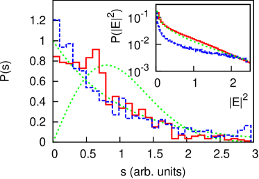
Figure 1: (Color online) Statistics of the eigenvalues of $\beta_{s}$ (red solid curve) and $\beta_{p}$ (blue dot-dashed curve) for $\alpha=\pi/15$. Dotted green lines shows Poissonian and Wigner distributions. In the inset, the statistics $P(|{\mathrm{\mathbf{E}}}|^{2})$ is shown (with the same denotations as in the main figure; dotted green line shows Porter-Thomas distribution).

For numerical computation of the eigenvalues and eigenfunctions of $\beta_{s}^{ijklmn}$ it is transformed into a square matrix by introducing indices $I=i+2k+2(N_{\mathrm{max}}-N_{\mathrm{min}}+1)m$, $J=j+2l+2(N_{\mathrm{max}}-N_{\mathrm{min}}+1)n$, where $N_{\mathrm{max}}$ and $N_{\mathrm{min}}$ are the maximal and minimal waveguide mode numbers, defining a cut-off for high- and low- order modes. Physically, cut-off for high-order modes is necessary because they are not guided anymore in transverse direction. On the other hand, if we consider the structures formed from the modes which are sufficiently far from $k_{\bot}=0$, very low order modes can be also neglected. For the simulations the values of $N_{\mathrm{max}}=30$, $N_{\mathrm{min}}=10$ were taken. In this case the matrix $\beta_{s}^{I,J}$ has the size $\sim 1000\times 1000$. Typical VCSEL parameters were used in simulations, in particular, the intracavity anisotropy $\gamma_{a}=0.1$ ns^-1, $\gamma_{p}=30$ ns^-1 were taken. The detuning $\delta$ of the cavity resonance from the gain line center (which enters to $\Upsilon$) controls the values of $k_{\bot}$ which have maximal gain sanmiguel95b . It is chosen large enough so that the modes with $k_{\bot}$ above the high-$k_{\bot}$ cut-off are preferred in the infinite device. Due to presence of the cut-off, ${\mathrm{\mathbf{k}}}_{\bot}$ near diagonal $|k_{x}|=|k_{y}|$ are selected at threshold babushkin08b ; schulz-ruhtenberg08 .

The statistics $P(s)$ of nearest neighbor separation $s_{i}\sim E_{i+1}-E_{i}$ of the eigenvalues $E_{i}$ of the matrices $\beta_{s}$ and $\beta_{p}$ is presented in Fig. 1 in comparison to Poissonian ($P(s)=e^{-s}$) and Wigner ($P(s)=\frac{\pi}{2}e^{-\pi s^{2}/4}$) distributions. The anisotropy axes in Fig. 1 are assumed to be rotated to a small angle $\alpha=\pi/15$ in respect to $x$-axis (such small displacement may also exist in real devices schulz-ruhtenberg08 , although in tendency the anisotropy is aligned to the boundaries). In this case, noticeable deviation from the Poissonian statistic is present for $\beta_{s}$. On the other hand, the eigenvalues of $\beta_{p}$ obey Poissonian statistics for every $\alpha$. In contrast, for $\alpha=0$, the deviation of $P(S)$ from the Poissonian distribution for $\beta_{s}$ is not noticeable anymore ( not shown in Fig. 1). This shows, that although PTC itself plays a critical role in the statistics of eigenvalues, the alignment of the intracavity anisotropy to the boundaries is also important, as it increases the degree of mode mixing produced by PTC.

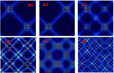
Figure 2: (Color online) Example of scared (a)–(e) as well as non-localized (f) eigenfunctions of $\beta_{s}$. In (a)–(c) $|E_{x}|^{2}$, $|E_{y}|^{2}$ and the intensity $I$ of the eigenfunction at threshold (i. e. having the lowest losses) are shown; in (d)–(f) the intensity $I$ distribution of some subsequent modes is presented.

Another important property of the operator $\beta_{s}$ (both for $\alpha>0$ and $\alpha=0$) is the presence of eigenfunctions localized along classical trajectories (i. e. SLS). Examples of such structures are shown in Fig. 2(a)-(e). In particular, in Fig. 2(a)-(c) the amplitudes of $x$- and $y$-polarization components as well as the full intensity of the mode at threshold (i. e. one with lowest losses) are shown. The mode in Fig. 2(c) is localized along tree different classical trajectories. It is interesting that particular polarization components, in contrast to the full intensity, are not localized along the complete trajectory in this case. Similar phenomena were observed also experimentally schulz-ruhtenberg08 (cf. also chen03a where different polarizations follow different trajectories).

In general, SLS are very common for $\beta_{s}$, for both $\alpha=0$ and $\alpha>0$ (see some further examples in Fig. 2(d), (e)). As a rule, they contain more than one classical trajectory. Like bogomolny04 ; bogomolny06 , SLS in our system seemingly do not become more rear with increasing of $k_{\bot}$. On the other hand, far from threshold the eigenfunctions becomes less localized (see an example in Fig. 2(f)).

The existence of SLS clearly points out to deviation from the full integrability, because the later assumes an existence of coordinate system where the billiard becomes fully separable, which excludes the possibility of SLS. For $\alpha=0$ this deviation is “undetected” by $P(s)$.

In contrast to $\beta_{s}$, the set of eigenfunctions of $\beta_{p}$ do not contain SLS. For $\alpha=0$, $\beta_{p}$ is diagonal. For $\alpha\neq 0$ it consists of $2\times 2$ blocks at the main diagonal (describing the polarization degrees of freedom). Therefore, all the cases we consider can be arranged in order of increasing of “nonintegrability”: $\beta_{p}$ with $\alpha=0$ is the most regular (and corresponds to the fully integrable case), whereas $\beta_{s}$ with $\alpha\neq 0$ is the most “nonintegrable”.

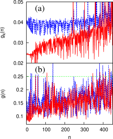
Figure 3: (Color online) Localization $g_{k}$ (in momentum space) (a) and $g$ (in coordinate space) (b) of the eigenfunctions of $\beta_{s}$ for $\alpha=\pi/15$ (red solid line) and for $\alpha=0$ (blue dashed line) arranged according increasing of the absolute values of the imaginary parts of corresponding eigenvalues (i. e. losses). In (b) $g$ is also shown for $\beta_{p}$ and $\alpha=0$ (dotted green line).

As follows from the previous, the shape of eigenmodes can provide a sensitive tool for the description of deviation of the system from the full integrability. This is supported by consideration of the statistics of eigenfunction amplitudes $P(|{\mathrm{\mathbf{E}}}|^{2})$ shown in inset to Fig. 1. $P(|{\mathrm{\mathbf{E}}}|^{2})$ for $\beta_{s}$ for both $\alpha\neq 0$ and $\alpha=0$ (they are very simular to each other and shown by a single red curve in the inset) is sufficiently different to the statistics of $\beta_{p}$ (blue curve). Remarkably, $P(|{\mathrm{\mathbf{E}}}|^{2})$ for $\beta_{s}$ is very close to Porter-Thomas distribution $P(|{\mathrm{\mathbf{E}}}|^{2})=e^{-|{\mathrm{\mathbf{E}}}|^{2}/2}/\sqrt{2\pi|{\mathrm{\mathbf{E}}}|^{2}}$ (which is characteristic for chaotic billiards stoeckmann99 ).

In this paper however, we are interested in analysis not only of different “levels of integrability”, but also of the localization properties of eigenfunctions. As it was shown in backer99 ; chen03d ; huang02 , sometimes the good indication of SLS is a localization in the “momentum” space ${\mathrm{\mathbf{k}}}_{\bot}$: $g_{k}=\Delta H_{0}/\langle H_{0}\rangle$, where $H_{0}=k_{\bot}^{2}$, $\Delta H_{0}=\sqrt{\langle H_{0}^{2}\rangle-\langle H_{0}\rangle^{2}}$. $g_{k}$ becomes exactly zero for the integrable case and is shown in Fig. 3(a) for $\beta_{s}$. One can see that $g_{k}$ is minimal at threshold ($n\sim 1$) in average for $\alpha\neq 0$, and grows with increasing losses ($n\rightarrow\infty$). For “less nonintegrable” case of $\alpha=0$ the localization level is nearly constant for low $n$, but starts to grow for $n$ above $\sim 200$. In general, $g_{k}$ can be used to distinguish between SLS and randomly-distributed eigenfunctions in chaotic billiards backer99 , but is not very well suitable for quasi-integrable billiards, because the modes unlocalized in coordinate space can be well localized in momentum space chen09 .

In this letter, we consider also a measure of localization in coordinate space. Namely, we introduce a functional $g[I(x,y)]=\int I\,dxdy/SI_{max}$ on the spatial intensity distribution $I(x,y)=|{\mathrm{\mathbf{E}}}(x,y)|^{2}$ (here the integration is made over the whole billiard area, and the result is normalized to the area $S$ and to the maximal value of the intensity $I_{max}=\mathrm{max}_{{\mathrm{\mathbf{r}}}_{\bot}}\left(I({\mathrm{\mathbf{r}}}_{\bot})\right)$. $g$ varies from one (for $I=\mathrm{const}$) to zero (for a pattern localized near a single point, i. e. for the one close to $\delta$-function). Remarkably, for an integrable square billiard $g=1/4$ for every eigenfunction (see Fig. 3(b), gree dashed curve). Therefore, deviation of $g$ from this value may indicate a deviation of the system from the complete integrability. In the other limit, for fully chaotic case, the typical value of $g$ is rather small. One can estimate it using the fact that eigenfunctions in fully chaotic billiards can be simulated as a sum of the waves with similar $k_{\bot}$ but random phases stoeckmann99 . For such a sum, according to our computations, the value of $g$ averaged over large number of eigenfunctions depends only on $k_{\bot}$ and is in the range of $0.06-0.07$ for $k_{\bot}$ used in the present article.

The values of $g$ for $\beta_{s}$ and $\beta_{p}$ are shown in Fig. 3. For the case of $\beta_{s}$ the deviation of $g$ from the “integrable” value $0.25$ is quite strong. Intriguingly, in analogy to $g_{k}$ the average value of $g$ grows with $n$. Thus, SLS appearing at threshold can be described as the patterns having lowest $g$ and $g_{k}$ simultaneously, supporting their consideration as coherent states chen02a ; chen03a ; chen03d . In general, the whole pair $\{g,g_{k}\}$ can be considered as a useful measure, allowing to distinguish between SLS, delocalized as well as “chaotic” structures.

It should be noted that the deviation from the full integrability in VCSEL disappears in a circular geometry gensty05 , because the terms $s$ and $\Upsilon$ in $\beta_{\infty}$ are isotropic in that case. In this sense, the situation is similar to the case of spin-orbit coupling of electrons in quantum dots berggren01 .

From the experimental point of view, it is rather problematic to distinguish clearly between the effects, appearing due to small deviations of the boundary conditions from a perfect square, and due to deviation of operator of the system $\hat{H}$ from the Laplacian. The result of the present article shows that the role of the former is often overestimated.

Whereas localization in the momentum space has a concrete physical reason in the case of VCSEL (certain ${\mathrm{\mathbf{k}}}_{\bot}$ have the highest gain because their frequencies are closer to the gain maximum), localization in the coordinate space is not obvious from the physical point of view. Even localization in the momentum space depends on the level of integrability of the system (regulated by $\alpha$), although the change of $\alpha$ does not affect the losses directly.

An intriguing similarity to the results of wiersig06 should be pointed out, despite the mechanism of emission in VCSEL is completely different from the one in dielectric microcavities. In wiersig06 , long lived states created by connection of the neighboring modes via continuum of external ones (i. e. mediated by dissipation) in the vicinity of ALC were shown to be localized in coordinate space. In contrast to wiersig06 , appearance of SLS in our system is related only to PTC and not to the presence of dissipation. Namely, according to our numerical simulations, if we remove all the losses in the system (i. e. assume $\kappa=0$ in $\beta_{\infty}$), SLS do not disappear. Moreover, the shape of many SLS is not altered significantly. Thus, the presence of dissipation does not create SLS but orders them instead. In addition, SLS are also not directly related to ALC in our case, because the frequencies of the modes grow in average monotonically with their losses, which is not the case in the vicinity of ALC.

In general, the results of this Letter together with wiersig06 ; ermann09 allows us to suspect a general mechanism, which is independent from every particular physical realization of open billiard, leading to a relation between localization and losses, which is still to be clarified.

The author is grateful for useful discussions with T. Ackemann.

References

- (1) H.-J. Stöckmann, Quantum Chaos: An Introduction (Cambridge University Press, New York, USA, 1999).
- (2) T. Guhr, A. Müller-Groeling, and H. A. Weidenmüller, Phys. Rep. 299, 189 (1998).
- (3) D. Ullmo, Rep. Progr. Phys. 71, 026001 (2007).
- (4) K.-F. Berggren and T. Ouchterlony, Found. Phys. 31, 233 (2001).
- (5) M. Novaes and M. A. M. de Aguiar, Phys. Rev. E 70, 045201 (2004).
- (6) K. Schaadt and A. Kudrolli, Phys. Rev. E 60, R3479 (1999).
- (7) K. F. Huang et al., Phys. Rev. Lett. 89, 224102 (2002).
- (8) T. Gensty et al., Phys. Rev. Lett. 94, 233901 (2005).
- (9) Y. F. Chen and K. F. Huang, Phys. Rev. E 68, 066207 (2003).
- (10) R. C. C. Chen et al., Opt. Lett. 34, 1810 (2009).
- (11) Y. F. Chen et al., Phys. Rev. E 68, 026210 (2003).
- (12) I. V. Babushkin et al., Phys. Rev. Lett. 100, 213901 (2008).
- (13) E. Bogomolny and C. Schmit, Phys. Rev. Lett. 93, 254102 (2004).
- (14) E. Bogomolny et al., Phys. Rev. Lett. 97, 254102 (2006).
- (15) M. A. Schulz-Ruhtenberg, Ph.D. thesis, Westfälische Wilhelms-Universität Mn̈ster, 2008.
- (16) Y. F. Chen, K. F. Huang, and Y. P. Lan, Phys. Rev. E 66, 046215 (2002).
- (17) Y. F. Chen et al., Phys. Rev. Lett. 90, 053904 (2003).
- (18) L. Ermann, G. G. Carlo, and M. Saraceno, Phys. Rev. Lett. 103, 054102 (2009).
- (19) J. Wiersig, Phys. Rev. Lett. 97, 253901 (2006).
- (20) N. A. Loiko and I. V. Babushkin, J. Opt. B: Quant. Semiclass. Opt. 3, S234 (2001).
- (21) M. S. Miguel, Q. Feng, and J. V. Moloney, Phys. Rev. A 52, 1728 (1995).
- (22) A. Backer and R. Schubert, J. Phys. A: Math. Gen. 32, 4795 (1999).