Hierarchical relational models for document networks

Abstract

We develop the relational topic model (RTM), a hierarchical model of both network structure and node attributes. We focus on document networks, where the attributes of each document are its words, that is, discrete observations taken from a fixed vocabulary. For each pair of documents, the RTM models their link as a binary random variable that is conditioned on their contents. The model can be used to summarize a network of documents, predict links between them, and predict words within them. We derive efficient inference and estimation algorithms based on variational methods that take advantage of sparsity and scale with the number of links. We evaluate the predictive performance of the RTM for large networks of scientific abstracts, web documents, and geographically tagged news.

and a1Work done while at Princeton University. a2Supported by ONR 175-6343, NSF CAREER 0745520 and grants from Google and Microsoft.

1 Introduction

Network data, such as citation networks of documents, hyperlinked networks of web pages, and social networks of friends, are pervasive in applied statistics and machine learning. The statistical analysis of network data can provide both useful predictive models and descriptive statistics. Predictive models can point social network members toward new friends, scientific papers toward relevant citations, and web pages toward other related pages. Descriptive statistics can uncover the hidden community structure underlying a network data set.

Recent research in this field has focused on latent variable models of link structure, models that decompose a network according to hidden patterns of connections between its nodes [Kemp, Griffiths and Tenenbaum (2004); Hofman and Wiggins (2007); Airoldi et al. (2008)]. These models represent a significant departure from statistical models of networks, which explain network data in terms of observed sufficient statistics [Fienberg, Meyer and Wasserman (1985); Wasserman and Pattison (1996); Getoor et al. (2001); Newman (2002); Taskar et al. (2004)].

While powerful, current latent variable models account only for the structure of the network, ignoring additional attributes of the nodes that might be available. For example, a citation network of articles also contains text and abstracts of the documents, a linked set of web-pages also contains the text for those pages, and an on-line social network also contains profile descriptions and other information about its members. This type of information about the nodes, along with the links between them, should be used for uncovering, understanding, and exploiting the latent structure in the data.

To this end, we develop a new model of network data that accounts for both links and attributes. While a traditional network model requires some observed links to provide a predictive distribution of links for a node, our model can predict links using only a new node’s attributes. Thus, we can suggest citations of newly written papers, predict the likely hyperlinks of a web page in development, or suggest friendships in a social network based only on a new user’s profile of interests. Moreover, given a new node and its links, our model provides a predictive distribution of node attributes. This mechanism can be used to predict keywords from citations or a user’s interests from his or her social connections. Such prediction problems are out of reach for traditional network models.

Here we focus on document networks. The attributes of each document are its text, that is, discrete observations taken from a fixed vocabulary, and the links between documents are connections such as friendships, hyperlinks, citations, or adjacency. To model the text, we build on previous research in mixed-membership document models, where each document exhibits a latent mixture of multinomial distributions or “topics” [Blei, Ng and Jordan (2003); Erosheva, Fienberg and Lafferty (2004); Steyvers and Griffiths (2007)]. The links are then modeled dependent on this latent representation. We call our model, which explicitly ties the content of the documents with the connections between them, the relational topic model (RTM).

The RTM affords a significant improvement over previously developed models of document networks. Because the RTM jointly models node attributes and link structure, it can be used to make predictions about one given the other. Previous work tends to explore one or the other of these two prediction problems. Some previous work uses link structure to make attribute predictions [Chakrabarti, Dom and Indyk (1998); Kleinberg (1999)], including several topic models [McCallum, Corrada-Emmanuel and Wang (2005); Wang, Mohanty and McCallum (2005); Dietz, Bickel and Scheffer (2007)]. However, none of these methods can make predictions about links given words.

Other models use node attributes to predict links [Hoff, Raftery and Handcock (2002)]. However, these models condition on the attributes but do not model them. While this may be effective for small numbers of attributes of low dimension, these models cannot make meaningful predictions about or using high-dimensional attributes such as text data. As our empirical study in Section 4 illustrates, the mixed-membership component provides dimensionality reduction that is essential for effective prediction.

In addition to being able to make predictions about links given words and words given links, the RTM is able to do so for new documents—documents outside of the training data. Approaches which generate document links through topic models treat links as discrete “terms” from a separate vocabulary that essentially indexes the observed documents [Cohn and Hofmann (2001); Erosheva, Fienberg and Lafferty (2004); Gruber, Rosen-Zvi and Weiss (2008); Nallapati and Cohen (2008); Sinkkonen, Aukia and Kaski (2008)]. Through this index, such approaches encode the observed training data into the model and thus cannot generalize to observations outside of them. Link and word predictions for new documents, of the kind we evaluate in Section 4.1, are ill defined.

Xu et al. (2006, 2008) have jointly modeled links and document content using nonparametric Bayesian techniques so as to avoid these problems. However, their work does not assume mixed-memberships, which have been shown to be useful for both document modeling [Blei, Ng and Jordan (2003)] and network modeling [Airoldi et al. (2008)]. Recent work from Nallapati et al. (2008) has also jointly modeled links and document content. We elucidate the subtle but important differences between their model and the RTM in Section 2.2. We then demonstrate in Section 4.1 that the RTM makes modeling assumptions that lead to significantly better predictive performance.

The remainder of this paper is organized as follows. First, we describe the statistical assumptions behind the relational topic model. Then, we derive efficient algorithms based on variational methods for approximate posterior inference, parameter estimation, and prediction. Finally, we study the performance of the RTM on scientific citation networks, hyperlinked web pages, and geographically tagged news articles. The RTM provides better word prediction and link prediction than natural alternatives and the current state of the art.

2 Relational topic models

The relational topic model (RTM) is a hierarchical probabilistic model of networks, where each node is endowed with attribute information. We will focus on text data, where the attributes are the words of the documents (see Figure 1). The RTM embeds this data in a latent space that explains both the words of the documents and how they are connected.

2.1 Modeling assumptions

The RTM builds on previous work in mixed-membership document models. Mixed-membership models are latent variable models of heterogeneous data, where each data point can exhibit multiple latent components. Mixed-membership models have been successfully applied in many domains, including survey data [Erosheva, Fienberg and Joutard (2007)], image data [Barnard et al. (2003); Fei-Fei and Perona (2005)], rank data [Gormley and Murphy (2009)], network data [Airoldi et al. (2008)] and document modeling [Blei, Ng and Jordan (2003); Steyvers and Griffiths (2007)]. Mixed-membership models were independently developed in the field of population genetics [Pritchard, Stephens and Donnelly (2000)].

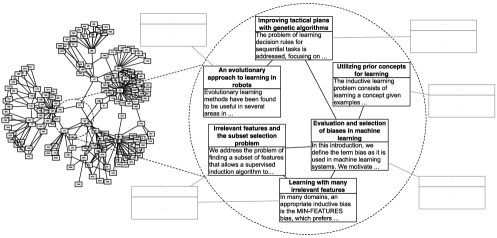
Figure 1: Example data appropriate for the relational topic model. Each document is represented as a bag of words and linked to other documents via citation. The RTM defines a joint distribution over the words in each document and the citation links between them.

To model node attributes, the RTM reuses the statistical assumptions behind latent Dirichlet allocation (LDA) [Blei, Ng and Jordan (2003)], a mixed-membership model of documents. Specifically, LDA is a hierarchical probabilistic model that uses a set of “topics,” distributions over a fixed vocabulary, to describe a corpus of documents. In its generative process, each document is endowed with a Dirichlet-distributed vector of topic proportions, and each word of the document is assumed drawn by first drawing a topic assignment from those proportions and then drawing the word from the corresponding topic distribution. While a traditional mixture model of documents assumes that every word of a document arises from a single mixture component, LDA allows each document to exhibit multiple components via the latent topic proportions vector.

In the RTM, each document is first generated from topics as in LDA. The links between documents are then modeled as binary variables, one for each pair of documents. These binary variables are distributed according to a distribution that depends on the topics used to generate each of the constituent documents. Because of this dependence, the content of the documents is statistically connected to the link structure between them. Thus, each document’s mixed-membership depends both on the content of the document as well as the pattern of its links. In turn, documents whose memberships are similar will be more likely to be connected under the model.

The parameters of the RTM are as follows: the topics $\bolds{\beta}_{1:K}$, $K$ multinomial parameters each describing a distribution on words; a $K$-dimensional Dirichlet parameter $\alpha$; and a function $\psi$ that provides binary probabilities. (This function is explained in detail below.) We denote a set of observed documents by $w_{1:D,1:N}$, where $w_{i,1:N}$ are the words of the $i$th document. (Words are assumed to be discrete observations from a fixed vocabulary.) We denote the links between the documents as binary variables $y_{1:D,1:D}$, where $y_{i,j}$ is one if there is a link between the $i$th and $j$th document. The RTM assumes that a set of observed documents $w_{1:D,1:N}$ and binary links between them $y_{1:D,1:D}$ are generated by the following process:

1. For each document $d$:

   1. Draw topic proportions $\theta_{d}|\alpha\sim\operatorname{Dir}(\alpha).$

   2. For each word $w_{d,n}$:

      1. Draw assignment $z_{d,n}|\theta_{d}\sim\operatorname{Mult}(\theta_{d})$.

      2. Draw word $w_{d,n}|z_{d,n},\bolds{\beta}_{1:K}\sim\operatorname{Mult}(\bolds{\beta}_{z_{d,n}}).$

2. For each pair of documents $d$, $d^{\prime}$:

   1. Draw binary link indicator

      $$y_{d,d^{\prime}}|\mathbf{z}_{d},\mathbf{z}_{d^{\prime}}\sim\psi(\cdot|\mathbf{z}_{d},\mathbf{z}_{d^{\prime}},\bolds{\eta}),$$

      where $\mathbf{z}_{d}=\{z_{d,1},z_{d,2},\ldots,z_{d,n}\}$.

Figure 2 illustrates the graphical model for this process for a single pair of documents. The full model, which is difficult to illustrate in a small graphical model, contains the observed words from all $D$ documents, and $D^{2}$ link variables for each possible connection between them.

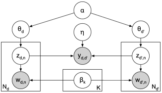
Figure 2: A two-document segment of the RTM. The variable $y_{d,d^{\prime}}$ indicates whether the two documents are linked. The complete model contains this variable for each pair of documents. This binary variable is generated contingent on the topic assignments for the participating documents, $\mathbf{z}_{d}$ and $\mathbf{z}_{d^{\prime}}$, and global regression parameters $\bolds{\eta}$. The plates indicate replication. This model captures both the words and the link structure of the data shown in Figure 1.

2.2 Link probability function

The function $\psi$ is the link probability function that defines a distribution over the link between two documents. This function is dependent on the two vectors of topic assignments that generated their words, $\mathbf{z}_{d}$ and $\mathbf{z}_{d^{\prime}}$.

This modeling decision is important. A natural alternative is to model links as a function of the topic proportions vectors $\theta_{d}$ and $\theta_{d^{\prime}}$. One such model is that of Nallapati et al. (2008), which extends the mixed-membership stochastic blockmodel [Airoldi et al. (2008)] to generate node attributes. Similar in spirit is the nongenerative model of Mei et al. (2008) which “regularizes” topic models with graph information. The issue with these formulations is that the links and words of a single document are possibly explained by disparate sets of topics, thereby hindering their ability to make predictions about words from links and vice versa.

In enforcing that the link probability function depends on the latent topic assignments $\mathbf{z}_{d}$ and $\mathbf{z}_{d^{\prime}}$, we enforce that the specific topics used to generate the links are those used to generate the words. A similar mechanism is employed in Blei and McAuliffe (2007) for nonpair-wise response variables. In estimating parameters, this means that the same topic indices describe both patterns of recurring words and patterns in the links. The results in Section 4.1 show that this provides a superior prediction mechanism.

We explore four specific possibilities for the link probability function. First, we consider

$$\psi_{\sigma}(y=1)=\sigma\bigl{(}{\bolds{\eta}}^{\mathrm{T}}(\overline{\mathbf{z}}_{d}\circ\overline{\mathbf{z}}_{d^{\prime}})+\nu\bigr{)},$$ (1)

where $\overline{\mathbf{z}}_{d}=\frac{1}{N_{d}}\sum_{n}z_{d,n}$, the $\circ$ notation denotes the Hadamard (element-wise) product, and the function $\sigma$ is the sigmoid. This link function models each per-pair binary variable as a logistic regression with hidden covariates. It is parameterized by coefficients $\eta$ and intercept $\nu$. The covariates are constructed by the Hadamard product of $\overline{\mathbf{z}}_{d}$ and $\overline{\mathbf{z}}_{d^{\prime}}$, which captures similarity between the hidden topic representations of the two documents.

Second, we consider

$$\psi_{e}(y=1)=\exp\bigl{(}{\bolds{\eta}}^{\mathrm{T}}(\overline{\mathbf{z}}_{d}\circ\overline{\mathbf{z}}_{d^{\prime}})+\nu\bigr{)}.$$ (2)

Here, $\psi_{e}$ uses the same covariates as $\psi_{\sigma}$, but has an exponential mean function instead. Rather than tapering off when $\overline{\mathbf{z}}_{d}$ and $\overline{\mathbf{z}}_{d^{\prime}}$ are close (i.e., when their weighted inner product, ${\bolds{\eta}}^{\mathrm{T}}(\overline{\mathbf{z}}_{d}\circ\overline{\mathbf{z}}_{d^{\prime}})$, is large), the probabilities returned by this function continue to increase exponentially. With some algebraic manipulation, the function $\psi_{e}$ can be viewed as an approximate variant of the modeling methodology presented in Blei and Jordan (2003).

Third, we consider

$$\psi_{\Phi}(y=1)=\Phi\bigl{(}{\bolds{\eta}}^{\mathrm{T}}(\overline{\mathbf{z}}_{d}\circ\overline{\mathbf{z}}_{d^{\prime}})+\nu\bigr{)},$$ (3)

where $\Phi$ represents the cumulative distribution function of the Normal distribution. Like $\psi_{\sigma}$, this link function models the link response as a regression parameterized by coefficients $\eta$ and intercept $\nu$. The covariates are also constructed by the Hadamard product of $\overline{\mathbf{z}}_{d}$ and $\overline{\mathbf{z}}_{d^{\prime}}$, but instead of the logit model hypothesized by $\psi_{\sigma}$, $\psi_{\Phi}$ models the link probability with a probit model.

Finally, we consider

$$\psi_{N}(y=1)=\exp\bigl{(}-{\bolds{\eta}}^{\mathrm{T}}(\overline{\mathbf{z}}_{d}-\overline{\mathbf{z}}_{d^{\prime}})\circ(\overline{\mathbf{z}}_{d}-\overline{\mathbf{z}}_{d^{\prime}})-\nu\bigr{)}.$$ (4)

Note that $\psi_{N}$ is the only one of the link probability functions which is not a function of $\overline{\mathbf{z}}_{d}\circ\overline{\mathbf{z}}_{d^{\prime}}$. Instead, it depends on a weighted squared Euclidean difference between the two latent topic assignment distributions. Specifically, it is the multivariate Gaussian density function, with mean 0 and diagonal covariance characterized by $\bolds{\eta}$, applied to $\overline{\mathbf{z}}_{d}-\overline{\mathbf{z}}_{d^{\prime}}$. Because the range of $\overline{\mathbf{z}}_{d}-\overline{\mathbf{z}}_{d^{\prime}}$ is finite, the probability of a link, $\psi_{N}(y=1)$, is also finite. We constrain the parameters $\bolds{\eta}$ and $\nu$ to ensure that it is between zero and one.

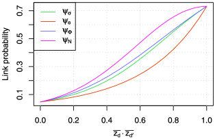
Figure 3: A comparison of different link probability functions. The plot shows the probability of two documents being linked as a function of their similarity (as measured by the inner product of the two documents’ latent topic assignments). All link probability functions were parameterized so as to have the same endpoints.

All four of the $\psi$ functions we consider are plotted in Figure 3. The link likelihoods suggested by the link probability functions are plotted against the inner product of $\overline{\mathbf{z}}_{d}$ and $\overline{\mathbf{z}}_{d^{\prime}}$. The parameters of the link probability functions were chosen to ensure that all curves have the same endpoints. Both $\psi_{\sigma}$ and $\psi_{\Phi}$ have similar sigmoidal shapes. In contrast, the $\psi_{e}$ is exponential in shape and its slope remains large at the right limit. The one-sided Gaussian form of $\psi_{N}$ is also apparent.

3 Inference, estimation and prediction

With the model defined, we turn to approximate posterior inference, parameter estimation, and prediction. We develop a variational inference procedure for approximating the posterior. We use this procedure in a variational expectation-maximization (EM) algorithm for parameter estimation. Finally, we show how a model whose parameters have been estimated can be used as a predictive model of words and links.

3.1 Inference

The goal of posterior inference is to compute the posterior distribution of the latent variables conditioned on the observations. As with many hierarchical Bayesian models of interest, exact posterior inference is intractable and we appeal to approximate inference methods. Most previous work on latent variable network modeling has employed Markov Chain Monte Carlo (MCMC) sampling methods to approximate the posterior of interest [Hoff, Raftery and Handcock (2002); Kemp, Griffiths and Tenenbaum (2004)]. Here, we employ variational inference [Jordan et al. (1999); Wainwright and Jordan (2005)], a deterministic alternative to MCMC sampling that has been shown to give comparative accuracy to MCMC with improved computational efficiency [Blei and Jordan (2006); Braun and McAuliffe (2007)]. Wainwright and Jordan (2008) investigate the properties of variational approximations in detail. Recently, variational methods have been employed in other latent variable network models [Hofman and Wiggins (2007); Airoldi et al. (2008)].

In variational methods, we posit a family of distributions over the latent variables, indexed by free variational parameters. Those parameters are then fit to be close to the true posterior, where closeness is measured by relative entropy. For the RTM, we use the fully-factorized family, where the topic proportions and all topic assignments are considered independent,

$$q(\bolds{\Theta},\mathbf{Z}|\bolds{\gamma},\bolds{\Phi})=\prod_{d}\biggl{[}q_{\theta}(\theta_{d}|\gamma_{d})\prod_{n}q_{z}(z_{d,n}|\phi_{d,n})\biggr{]}.$$ (5)

The parameters $\bolds{\gamma}$ are variational Dirichlet parameters, one for each document, and $\bolds{\Phi}$ are variational multinomial parameters, one for each word in each document. Note that $\mathbb{E}_{q}[z_{d,n}]=\phi_{d,n}$.

Minimizing the relative entropy is equivalent to maximizing the Jensen’s lower bound on the marginal probability of the observations, that is, the evidence lower bound (ELBO),

$$\hskip 18.0pt\mathscr{L} = \sum_{(d_{1},d_{2})}\mathbb{E}_{q}[\log p(y_{d_{1},d_{2}}|\mathbf{z}_{d_{1}},\mathbf{z}_{d_{2}},\bolds{\eta},\nu)]+\sum_{d}\sum_{n}\mathbb{E}_{q}[\log p(z_{d,n}|\bolds{\theta}_{d})]$$

$${}+\sum_{d}\sum_{n}\mathbb{E}_{q}[\log p(w_{d,n}|\bolds{\beta}_{1:K},z_{d,n})]+\sum_{d}\mathbb{E}_{q}[\log p(\bolds{\theta}_{d}|\alpha)]+\mathrm{H}(q),$$

where $(d_{1},d_{2})$ denotes all document pairs and $\mathrm{H}(q)$ denotes the entropy of the distribution $q$. The first term of the ELBO differentiates the RTM from LDA [Blei, Ng and Jordan (2003)]. The connections between documents affect the objective in approximate posterior inference (and, below, in parameter estimation).

We develop the inference procedure below under the assumption that only observed links will be modeled (i.e., $y_{d_{1},d_{2}}$ is either $1$ or unobserved). We do this for both methodological and computational reasons.

First, while one can fix $y_{d_{1},d_{2}}=1$ whenever a link is observed between $d_{1}$ and $d_{2}$ and set $y_{d_{1},d_{2}}=0$ otherwise, this approach is inappropriate in corpora where the absence of a link cannot be construed as evidence for $y_{d_{1},d_{2}}=0$. In these cases, treating these links as unobserved variables is more faithful to the underlying semantics of the data. For example, in large social networks such as Facebook the absence of a link between two people does not necessarily mean that they are not friends; they may be real friends who are unaware of each other’s existence in the network. Treating this link as unobserved better respects our lack of knowledge about the status of their relationship.

Second, treating nonlinks links as hidden decreases the computational cost of inference; since the link variables are leaves in the graphical model, they can be removed whenever they are unobserved. Thus, the complexity of computation scales linearly with the number of observed links rather than the number of document pairs. When the number of true observations is sparse relative to the number of document pairs, as is typical, this provides a significant computational advantage. For example, on the Cora data set described in Section 4, there are 3,665,278 unique document pairs but only 5278 observed links. Treating nonlinks as hidden in this case leads to an inference procedure which is nearly 700 times faster.

Our aim now is to compute each term of the objective function given in equation (3.1). The first term,

$$\sum_{(d_{1},d_{2})}\mathscr{L}_{d_{1},d_{2}}\equiv\sum_{(d_{1},d_{2})}\mathbb{E}_{q}[\log p(y_{d_{1},d_{2}}|\mathbf{z}_{d_{1}},\mathbf{z}_{d_{2}},\bolds{\eta},\nu)],$$ (7)

depends on our choice of link probability function. For many link probability functions, this term cannot be expanded analytically. However, if the link probability function depends only on $\overline{\mathbf{z}}_{d_{1}}\circ\overline{\mathbf{z}}_{d_{2}}$, we can expand the expectation using the following first-order approximation [Braun and McAuliffe (2007)]:

$$\mathscr{L}_{(d_{1},d_{2})}=\mathbb{E}_{q}[\log\psi(\overline{\mathbf{z}}_{d_{1}}\circ\overline{\mathbf{z}}_{d_{2}})]\approx\log\psi(\mathbb{E}_{q}[\overline{\mathbf{z}}_{d_{1}}\circ\overline{\mathbf{z}}_{d_{2}}])=\log\psi(\overline{\bolds{\pi}}_{d_{1},d_{2}}),$$

where $\overline{\bolds{\pi}}_{d_{1},d_{2}}=\overline{\bolds{\phi}}_{d_{1}}\circ\overline{\bolds{\phi}}_{d_{2}}$ and $\overline{\bolds{\phi}}_{d}=\mathbb{E}_{q}[\overline{\mathbf{z}}_{d}]=\frac{1}{N_{d}}\sum_{n}\phi_{d,n}$. In this work, we explore three functions which can be written in this form,

$$\mathbb{E}_{q}[\log\psi_{\sigma}(\overline{\mathbf{z}}_{d_{1}}\circ\overline{\mathbf{z}}_{d_{2}})] \approx \log\sigma({\bolds{\eta}}^{\mathrm{T}}\overline{\bolds{\pi}}_{d_{1},d_{2}}+\nu),$$

$$\mathbb{E}_{q}[\log\psi_{\Phi}(\overline{\mathbf{z}}_{d_{1}}\circ\overline{\mathbf{z}}_{d_{2}})] \approx \log\Phi({\bolds{\eta}}^{\mathrm{T}}\overline{\bolds{\pi}}_{d_{1},d_{2}}+\nu),$$ (8)

$$\mathbb{E}_{q}[\log\psi_{e}(\overline{\mathbf{z}}_{d_{1}}\circ\overline{\mathbf{z}}_{d_{2}})] = {\bolds{\eta}}^{\mathrm{T}}\overline{\bolds{\pi}}_{d_{1},d_{2}}+\nu.$$

Note that for $\psi_{e}$ the expression is exact. The likelihood when $\psi_{N}$ is chosen as the link probability function can also be computed exactly,

$$\mathbb{E}_{q}[\log\psi_{N}(\overline{\mathbf{z}}_{d_{1}},\overline{\mathbf{z}}_{d_{2}})]=-\nu-\sum_{i}\eta_{i}\bigl{(}(\overline{\bolds{\phi}}_{d_{1},i}-\overline{\bolds{\phi}}_{d_{2},i})^{2}+\operatorname{Var}(\overline{\mathbf{z}}_{d_{1},i})+\operatorname{Var}(\overline{\mathbf{z}}_{d_{2},i})\bigr{)},$$

where $\overline{\mathbf{z}}_{d,i}$ denotes the $i$th element of the mean topic assignment vector, $\overline{\mathbf{z}}_{d}$, and $\operatorname{Var}(\overline{\mathbf{z}}_{d,i})=\frac{1}{N_{d}^{2}}\sum_{n}\phi_{d,n,i}(1-\phi_{d,n,i})$, where $\phi_{d,n,i}$ is the $i$th element of the multinomial parameter $\phi_{d,n}$. (See Appendix A.)

Leveraging these expanded expectations, we then use coordinate ascent to optimize the ELBO with respect to the variational parameters $\bolds{\gamma},\bolds{\Phi}$. This yields an approximation to the true posterior. The update for the variational multinomial $\phi_{d,j}$ is

$$\phi_{d,j}\propto\exp\biggl{\{}\sum_{d^{\prime}\neq d}\nabla_{\phi_{d,n}}\mathscr{L}_{d,d^{\prime}}+\mathbb{E}_{q}[\log\theta_{d}|\gamma_{d}]+\log\bolds{\beta}_{\cdot,w_{d,j}}\biggr{\}}.$$ (9)

The contribution to the update from link information, $\nabla_{\phi_{d,n}}\mathscr{L}_{d,d^{\prime}}$, depends on the choice of link probability function. For the link probability functions expanded in equation (3.1), this term can be written as

$$\nabla_{\phi_{d,n}}\mathscr{L}_{d,d^{\prime}}=(\nabla_{\overline{\bolds{\pi}}_{d_{1},d_{2}}}\mathscr{L}_{d,d^{\prime}})\circ\frac{\overline{\bolds{\phi}}_{d^{\prime}}}{N_{d}}.$$ (10)

Intuitively, equation (10) will cause a document’s latent topic assignments to be nudged in the direction of neighboring documents’ latent topic assignments. The magnitude of this pull depends only on $\overline{\bolds{\pi}}_{d,d^{\prime}}$, that is, some measure of how close they are already. The corresponding gradients for the functions in equation (3.1) are

$$\nabla_{\overline{\bolds{\pi}}_{d,d^{\prime}}}\mathscr{L}^{\sigma}_{d,d^{\prime}} \approx \bigl{(}1-\sigma({\bolds{\eta}}^{\mathrm{T}}\overline{\bolds{\pi}}_{d,d^{\prime}}+\nu)\bigr{)}\bolds{\eta},$$

$$\nabla_{\overline{\bolds{\pi}}_{d,d^{\prime}}}\mathscr{L}^{\Phi}_{d,d^{\prime}} \approx \frac{\Phi^{\prime}({\bolds{\eta}}^{\mathrm{T}}\overline{\bolds{\pi}}_{d,d^{\prime}}+\nu)}{\Phi({\bolds{\eta}}^{\mathrm{T}}\overline{\bolds{\pi}}_{d,d^{\prime}}+\nu)}\bolds{\eta},$$

$$\nabla_{\overline{\bolds{\pi}}_{d,d^{\prime}}}\mathscr{L}^{e}_{d,d^{\prime}} = \bolds{\eta}.$$

The gradient when $\psi_{N}$ is the link probability function is

$$\nabla_{\phi_{d,n}}\mathscr{L}^{N}_{d,d^{\prime}}=\frac{2}{N_{d}}\bolds{\eta}\circ\biggl{(}\overline{\bolds{\phi}}_{d^{\prime}}-\overline{\bolds{\phi}}_{d,-n}-\frac{\mathbf{1}}{N_{d}}\biggr{)},$$ (11)

where $\overline{\bolds{\phi}}_{d,-n}=\overline{\bolds{\phi}}_{d}-\frac{1}{N_{d}}\phi_{d,n}$. Similar in spirit to equation (10), equation (11) will cause a document’s latent topic assignments to be drawn toward those of its neighbors. This draw is tempered by $\overline{\bolds{\phi}}_{d,-n}$, a measure of how similar the current document is to its neighbors.

The contribution to the update in equation (9) from the word evidence $\log\bolds{\beta}_{\cdot,w_{d,j}}$ can be computed by taking the element-wise logarithm of the $w_{d,j}$th column of the topic matrix $\bolds{\beta}$. The contribution to the update from the document’s latent topic proportions is given by

$$\mathbb{E}_{q}[\log\bolds{\theta}_{d}|\bolds{\gamma}_{d}]=\Psi(\bolds{\gamma}_{d})-\Psi\Bigl{(}\sum\gamma_{d,i}\Bigr{)},$$

where $\Psi$ is the digamma function. (A digamma of a vector is the vector of digammas.) The update for $\bolds{\gamma}$ is identical to that in variational inference for LDA [Blei, Ng and Jordan (2003)],

$$\gamma_{d}\leftarrow\alpha+\sum_{n}\bolds{\phi}_{d,n}.$$

These updates are fully derived in Appendix A.

3.2 Parameter estimation

We fit the model by finding maximum likelihood estimates for each of the parameters: multinomial topic vectors $\bolds{\beta}_{1:K}$ and link function parameters $\bolds{\eta},\nu$. Once again, this is intractable so we turn to an approximation. We employ variational expectation-maximization, where we iterate between optimizing the ELBO of equation (3.1) with respect to the variational distribution and with respect to the model parameters. This is equivalent to the usual expectation-maximization algorithm [Dempster, Laird and Rubin (1977)], except that the computation of the posterior is replaced by variational inference.

Optimizing with respect to the variational distribution is described in Section 3.1. Optimizing with respect to the model parameters is equivalent to maximum likelihood estimation with expected sufficient statistics, where the expectation is taken with respect to the variational distribution.

The update for the topics matrix $\bolds{\beta}$ is

$$\beta_{k,w}\propto\sum_{d}\sum_{n}\mathbh{1}(w_{d,n}=w)\phi_{d,n,k}.$$ (12)

This is the same as the variational EM update for LDA [Blei, Ng and Jordan (2003)]. In practice, we smooth our estimates of $\beta_{k,w}$ using pseudocount smoothing [Jurafsky and Martin (2008)] which helps to prevent overfitting by positing a Dirichlet prior on $\bolds{\beta}_{k}$.

In order to fit the parameters $\bolds{\eta},\nu$ of the logistic function of equation (1), we employ gradient-based optimization. Using the approximation described in equation (3.1), we compute the gradient of the objective given in equation (3.1) with respect to these parameters,

$$\nabla_{\bolds{\eta}}\mathscr{L} \approx \sum_{(d_{1},d_{2})}[y_{d_{1},d_{2}}-\sigma({\bolds{\eta}}^{\mathrm{T}}\overline{\bolds{\pi}}_{d_{1},d_{2}}+\nu)]\overline{\bolds{\pi}}_{d_{1},d_{2}},$$

$$\frac{\partial}{\partial\nu}\mathscr{L} \approx \sum_{(d_{1},d_{2})}[y_{d_{1},d_{2}}-\sigma({\bolds{\eta}}^{\mathrm{T}}\overline{\bolds{\pi}}_{d_{1},d_{2}}+\nu)].$$

Note that these gradients cannot be used to directly optimize the parameters of the link probability function without negative observations (i.e., $y_{d_{1},d_{2}}=0$). We address this by applying a regularization penalty. This regularization penalty along with parameter update procedures for the other link probability functions are given in Appendix B.

3.3 Prediction

With a fitted model, our ultimate goal is to make predictions about new data. We describe two kinds of prediction: link prediction from words and word prediction from links.

In link prediction, we are given a new document (i.e., a document which is not in the training set) and its words. We are asked to predict its links to the other documents. This requires computing

$$p(y_{d,d^{\prime}}|\mathbf{w_{d}},\mathbf{w_{d^{\prime}}})=\sum_{\mathbf{z}_{d},\mathbf{z}_{d^{\prime}}}p(y_{d,d^{\prime}}|\overline{\mathbf{z}}_{d},\overline{\mathbf{z}}_{d^{\prime}})p(\mathbf{z}_{d},\mathbf{z}_{d^{\prime}}|\mathbf{w_{d}},\mathbf{w_{d^{\prime}}}),$$

an expectation with respect to a posterior that we cannot compute. Using the inference algorithm from Section 3.1, we find variational parameters which optimize the ELBO for the given evidence, that is, the words and links for the training documents and the words in the test document. Replacing the posterior with this approximation $q(\bolds{\Theta},\mathbf{Z})$, the predictive probability is approximated with

$$p(y_{d,d^{\prime}}|\mathbf{w_{d}},\mathbf{w_{d^{\prime}}})\approx\mathbb{E}_{q}[p(y_{d,d^{\prime}}|\overline{\mathbf{z}}_{d},\overline{\mathbf{z}}_{d^{\prime}})].$$ (13)

In a variant of link prediction, we are given a new set of documents (documents not in the training set) along with their words and asked to select the links most likely to exist. The predictive probability for this task is proportional to equation (13).

The second predictive task is word prediction, where we predict the words of a new document based only on its links. As with link prediction, $p(w_{d,i}|\mathbf{y_{d}})$ cannot be computed. Using the same technique, a variational distribution can approximate this posterior. This yields the predictive probability

$$p(w_{d,i}|\mathbf{y_{d}})\approx\mathbb{E}_{q}[p(w_{d,i}|z_{d,i})].$$

Note that models which treat the endpoints of links as discrete observations of data indices cannot participate in the two tasks presented here. They cannot make meaningful predictions for documents that do not appear in the training set [Cohn and Hofmann (2001); Erosheva, Fienberg and Lafferty (2004); Nallapati and Cohen (2008); Sinkkonen, Aukia and Kaski (2008)]. By modeling both documents and links generatively, our model is able to give predictive distributions for words given links, links given words, or any mixture thereof.

4 Empirical results

We examined the RTM on four data sets. Words were stemmed; stop words, that is, words like “and,” “of,” or “but,” and infrequently occurring words were removed. Directed links were converted to undirected links and documents with no links were removed. The Cora data [McCallum et al. (2000)] contains abstracts from the Cora computer science research paper search engine, with links between documents that cite each other. The WebKB data [Craven et al. (1998)] contains web pages from the computer science departments of different universities, with links determined from the hyperlinks on each page. The PNAS data contains recent abstracts from the Proceedings of the National Academy of Sciences. The links between documents are intra-PNAS citations. The LocalNews data set is a corpus of local news culled from various media markets throughout the United States. We create one bag-of-words document associated with each state (including the District of Columbia); each state’s “document” consists of headlines and summaries from local news in that state’s media markets. Links between states were determined by geographical adjacency. Summary statistics for these data sets are given in Table 1.

Table 1: Summary statistics for the four data sets after processing

Data set	# of documents	# of words	Number of links	Lexicon size
Cora	2708	0,49216	5278	1433
WebKB	0877	0,79365	1388	1703
PNAS	2218	11,9162	1577	2239
LocalNews	0051	0,93765	0107	1242

4.1 Evaluating the predictive distribution

As with any probabilisticmodel, the RTM defines a probability distribution over unseen data. After inferring the latent variables from data (as described in Section 3.1), we ask how well the model predicts the links and words of unseen nodes. Models that give higher probability to the unseen documents better capture the joint structure of words and links.

We study the RTM with three link probability functions discussed above: the logistic link probability function, $\psi_{\sigma}$, of equation (1); the exponential link probability function, $\psi_{e}$, of equation (2); and the probit link probability function, $\psi_{\Phi}$, of equation (3). We compare these models against two alternative approaches.

The first (“Pairwise Link-LDA”) is the model proposed by Nallapati et al. (2008), which is an extension of the mixed membership stochastic block model [Airoldi et al. (2008)] to model network structure and node attributes. This model posits that each link is generated as a function of two individual topics, drawn from the topic proportions vectors associated with the endpoints of the link. Because latent topics for words and links are drawn independently in this model, it cannot ensure that the discovered topics are representative of both words and links simultaneously. Additionally, this model introduces additional variational parameters for every link which adds computational complexity.

The second (“LDA $+$ Regression”) first fits an LDA model to the documents and then fits a logistic regression model to the observed links, with input given by the Hadamard product of the latent class distributions of each pair of documents. Rather than performing dimensionality reduction and regression simultaneously, this method performs unsupervised dimensionality reduction first, and then regresses to understand the relationship between the latent space and underlying link structure. All models were fit such that the total mass of the Dirichlet hyperparameter $\alpha$ was 1.0. (While we omit a full sensitivity study here, we observed that the performance of the models was similar for $\alpha$ within a factor of 2 above and below the value we chose.)

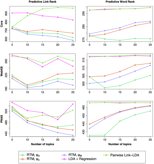
Figure 4: Average held-out predictive link rank (left) and word rank (right) as a function of the number of topics. Lower is better. For all three corpora, RTMs outperform baseline unigram, LDA and “Pairwise Link-LDA” Nallapati et al. (2008).

We measured the performance of these models on link prediction and word prediction (see Section 3.3). We divided the Cora, WebKB and PNAS data sets each into five folds. For each fold and for each model, we ask two predictive queries: given the words of a new document, how probable are its links; and given the links of a new document, how probable are its words? Again, the predictive queries are for completely new test documents that are not observed in training. During training the test documents are removed along with their attendant links. We show the results for both tasks in terms of predictive rank as a function of the number of topics in Figure 4. (See Section 5 for a discussion on potential approaches for selecting the number of topics and the Dirichlet hyperparameter $\alpha$.) Here we follow the convention that lower predictive rank is better.

In predicting links, the three variants of the RTM perform better than all of the alternative models for all of the data sets (see Figure 4, left column). Cora is paradigmatic, showing a nearly 40% improvement in predictive rank over baseline and 25% improvement over LDA $+$ Regression. The performance for the RTM on this task is similar for all three link probability functions. We emphasize that the links are predicted to documents seen in the training set from documents which were held out. By incorporating link and node information in a joint fashion, the model is able to generalize to new documents for which no link information was previously known.

Note that the performance of the RTM on link prediction generally increases as the number of topics is increased (there is a slight decrease on WebKB). In contrast, the performance of the Pairwise Link-LDA worsens as the number of topics is increased. This is most evident on Cora, where Pairwise Link-LDA is competitive with RTM at five topics, but the predictive link rank monotonically increases after that despite its increased dimensionality (and commensurate increase in computational difficulty). We hypothesize that Pairwise Link-LDA exhibits this behavior because it uses some topics to explain the words observed in the training set, and other topics to explain the links observed in the training set. This problem is exacerbated as the number of topics is increased, making it less effective at predicting links from word observations.

In predicting words, the three variants of the RTM again outperform all of the alternative models (see Figure 4, right column). This is because the RTM uses link information to influence the predictive distribution of words. In contrast, the predictions of LDA $+$ Regression and Pairwise Link-LDA barely use link information; thus, they give predictions independent of the number of topics similar to those made by a simple unigram model.

4.2 Automatic link suggestion

A natural real-world application of link prediction is to suggest links to a user based on the text of a document. One might suggest citations for an abstract or friends for a user in a social network.

As a complement to the quantitative evaluation of link prediction given in the previous section, Table 2 illustrates suggested citations using RTM ($\psi_{e}$) and LDA $+$ Regression as

Table 2: Top eight link predictions made by RTM ($\psi_{e}$) and LDA $+$ Regression for two documents (italicized) from Cora. The models were fit with 10 topics. Boldfaced titles indicate actual documents cited by or citing each document. Over the whole corpus, RTM improves precision over LDA $+$ Regression by 80% when evaluated on the first 20 documents retrieved

	Markov chain Monte Carlo convergence diagnostics: A comparative review
RTM ($\psi_{e}$)	Minorization conditions and convergence rates for Markov chain Monte Carlo
	Rates of convergence of the Hastings and Metropolis algorithms
	Possible biases induced by MCMC convergence diagnostics
	Bounding convergence time of the Gibbs sampler in Bayesian image restoration
	Self regenerative Markov chain Monte Carlo
	Auxiliary variable methods for Markov chain Monte Carlo with applications
	Rate of Convergence of the Gibbs Sampler by Gaussian Approximation
	Diagnosing convergence of Markov chain Monte Carlo algorithms
LDA $+$ Regression	Exact Bound for the Convergence of Metropolis Chains
	Self regenerative Markov chain Monte Carlo
	Minorization conditions and convergence rates for Markov chain Monte Carlo
	Gibbs–Markov models
	Auxiliary variable methods for Markov chain Monte Carlo with applications
	Markov Chain Monte Carlo Model Determination for Hierarchical and Graphical Models
	Mediating instrumental variables
	A qualitative framework for probabilistic inference
	Adaptation for Self Regenerative MCMC

	Competitive environments evolve better solutions for complex tasks
RTM ($\psi_{e}$)	Coevolving High Level Representations
	A Survey of Evolutionary Strategies
	Genetic Algorithms in Search, Optimization and Machine Learning
	Strongly typed genetic programming in evolving cooperation strategies
	Solving combinatorial problems using evolutionary algorithms
	A promising genetic algorithm approach to job-shop scheduling…
	Evolutionary Module Acquisition
	An Empirical Investigation of Multi-Parent Recombination Operators…
LDA $+$ Regression	A New Algorithm for DNA Sequence Assembly
	Identification of protein coding regions in genomic DNA
	Solving combinatorial problems using evolutionary algorithms
	A promising genetic algorithm approach to job-shop scheduling…
	A genetic algorithm for passive management
	The Performance of a Genetic Algorithm on a Chaotic Objective Function
	Adaptive global optimization with local search
	Mutation rates as adaptations

predictive models. These suggestions were computed from a model fit on one of the folds of the Cora data using 10 topics. (Results are qualitatively similar for models fit using different numbers of topics; see Section 5 for strategies for choosing the number of topics.) The top results illustrate suggested links for “Markov chain Monte Carlo convergence diagnostics: A comparative review,” which occurs in this fold’s training set. The bottom results illustrate suggested links for “Competitive environments evolve better solutions for complex tasks,” which is in the test set.

RTM outperforms LDA $+$ Regression in being able to identify more true connections. For the first document, RTM finds 3 of the connected documents versus 1 for LDA $+$ Regression. For the second document, RTM finds 3 while LDA $+$ Regression does not find any. This qualitative behavior is borne out quantitatively over the entire corpus. Considering the precision of the first 20 documents retrieved by the models, RTM improves precision over LDA $+$ Regression by 80%. (Twenty is a reasonable number of documents for a user to examine.)

While both models found several connections which were not observed in the data, those found by the RTM are qualitatively different. In the first document, both sets of suggested links are about Markov chain Monte Carlo. However, the RTM finds more documents relating specifically to convergence and stationary behavior of Monte Carlo methods. LDA $+$ Regression finds connections to documents in the milieu of MCMC, but many are only indirectly related to the input document. The RTM is able to capture that the notion of “convergence” is an important predictor for citations, and has adjusted the topic distribution and predictors correspondingly. For the second document, the documents found by the RTM are also of a different nature than those found by LDA $+$ Regression. All of the documents suggested by RTM relate to genetic algorithms. LDA $+$ Regression, however, suggests some documents which are about genomics. By relying only on words, LDA $+$ Regression conflates two “genetic” topics which are similar in vocabulary but different in citation structure. In contrast, the RTM partitions the latent space differently, recognizing that papers about DNA sequencing are unlikely to cite papers about genetic algorithms, and vice versa. Better modeling the properties of the network jointly with the content of the documents, the model is able to better tease apart the community structure.

4.3 Modeling spatial data

While explicitly linked structures like citation networks offer one sort of connectivity, data with spatial or temporal information offer another sort of connectivity. In this section we show how RTMs can be used to model spatially connected data by applying it to the LocalNews data set, a corpus of news headlines and summaries from each state, with document linkage determined by spatial adjacency.

Figure 5 shows the per state topic distributions inferred by RTM (left) and LDA (right). Both models were fit with five topics using the same initialization. (We restrict the discussion here to five topics for expositional convenience. See Section 5 for a discussion on potential approaches for selecting the number of topics.) While topics are, strictly speaking, exchangeable and therefore not comparable between models, using the same initialization typically yields topics which are amenable to comparison. Each row of Figure 5 shows a single component of each state’s topic proportion for RTM and LDA. That is, if $\theta_{s}$ is the latent topic proportions vector for state $s$, then $\theta_{s1}$ governs the intensity of that state’s color in the first row, $\theta_{s2}$ the second, and so on.

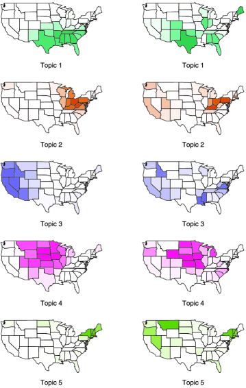
Figure 5: A comparison between RTM (left) and LDA (right) of topic distributions on local news data. Each color/row depicts a single topic. Each state’s color intensity indicates the magnitude of that topic’s component. The corresponding words associated with each topic are given in Table 3. Whereas LDA finds geographically diffuse topics, RTM, by modeling spatial connectivity, finds coherent regions.

While both RTM and LDA model the words in each state’s local news corpus, LDA ignores geographical information. Hence, it finds topics which are distributed over a wide swath of states which are often not contiguous. For example, LDA’s topic 1 is strongly expressed by Maine and Illinois, along with Texas and other states in the South and West. In contrast, RTM only assigns nontrivial mass to topic 1 in Southern states. Similarly, LDA finds that topic 5 is expressed by several states in the Northeast and the West. The RTM, however, concentrates topic 4’s mass on the Northeastern states.

Table 3: The top eight words in each RTM (left) and LDA (right) topic shown in Figure 5 ranked by score (defined below). RTM finds words which are predictive of both a state’s geography and its local news

The RTM does so by finding different topic assignments for each state and, commensurately, different distributions over words for each topic. Table 3 shows the top words in each RTM topic and each LDA topic. Words are ranked by the following score:

$$\mathrm{score}_{k,w}\equiv\beta_{k,w}\biggl{(}\log\beta_{k,w}-\frac{1}{K}\sum_{k^{\prime}}\log\beta_{k^{\prime},w}\biggr{)}.$$

The score finds words which are likely to appear in a topic, but also corrects for frequent words. The score therefore puts greater weight on words which more easily characterize a topic. Table 3 shows that RTM finds words more geographically indicative. While LDA provides one way of analyzing this collection of documents, the RTM enables a different approach which is geographically cognizant. For example, LDA’s topic 3 is an assortment of themes associated with California (e.g., “marriage”) as well as others (“scores,” “registration,” “schools”). The RTM, on the other hand, discovers words thematically related to a single news item (“measure,” “protesters,” “appeals”) local to California. The RTM typically finds groups of words associated with specific news stories, since they are easily localized, while LDA finds words which cut broadly across news stories in many states. Thus, on topic 5, the RTM discovers key words associated with news stories local to the Northeast such as “manslaughter” and “developer.” On topic 5, the RTM also discovers a peculiarity of the Northeastern dialect: that roads are given the appellation “route” more frequently than elsewhere in the country.

By combining textual information along with geographical information, the RTM provides a novel exploratory tool for identifying clusters of words that are driven by both word co-occurrence and geographic proximity. Note that the RTM finds regions in the United States which correspond to typical clusterings of states: the South, the Northeast, the Midwest, etc. Further, the soft clusterings found by RTM confirm many of our cultural intuitions—while New York is definitively a Northeastern state, Virginia occupies a liminal space between the MidAtlantic and the South.

5 Discussion

There are many avenues for future work on relational topic models. Applying the RTM to diverse types of “documents” such as protein-interaction networks or social networks, whose node attributes are governed by rich internal structure, is one direction. Even the text documents which we have focused on in this paper have internal structure such as syntax [Boyd-Graber and Blei (2008)] which we are discarding in the bag-of-words model. Augmenting and specializing the RTM to these cases may yield better models for many application domains.

As with any parametric mixed-membership model, the number of latent components in the RTM must be chosen using either prior knowledge or model-selection techniques such as cross-validation. Incorporating non-parametric Bayesian priors such as the Dirichlet process into the model would allow it to flexibly adapt the number of topics to the data [Ferguson (1973); Antoniak (1974); Kemp, Griffiths and Tenenbaum (2004); Teh et al. (2007)]. This, in turn, may give researchers new insights into the latent membership structure of networks.

In sum, the RTM is a hierarchical model of networks and per-node attribute data. The RTM is used to analyze linked corpora such as citation networks, linked web pages, social networks with user profiles, and geographically tagged news. We have demonstrated qualitatively and quantitatively that the RTM provides an effective and useful mechanism for analyzing and using such data. It significantly improves on previous models, integrating both node-specific information and link structure to give better predictions.

Appendix A Derivation of coordinate ascent updates

Inference under the variational method amounts to finding values of the variational parameters $\bolds{\gamma},\bolds{\Phi}$ which optimize the evidence lower bound, $\mathscr{L}$, given in equation (3.1). To do so, we first expand the expectations in these terms:

$$\mathscr{L} = \sum_{(d_{1},d_{2})}\mathscr{L}_{d_{1},d_{2}}+\sum_{d}\sum_{n}{\phi_{d,n}}^{\mathrm{T}}\log\beta_{\cdot,w_{d,n}}$$

$${}+\sum_{d}\sum_{n}{\phi_{d,n}}^{\mathrm{T}}\bigl{(}\Psi(\gamma_{d})-\mathbf{1}\Psi({\mathbf{1}}^{\mathrm{T}}\gamma_{d})\bigr{)}$$

$${}+\sum_{d}{(\alpha-1)}^{\mathrm{T}}\bigl{(}\Psi(\gamma_{d})-\mathbf{1}\Psi({\mathbf{1}}^{\mathrm{T}}\gamma_{d})\bigr{)}$$

$${}+\sum_{d}\sum_{n}{\phi_{d,n}}^{\mathrm{T}}\log\phi_{d,n}$$

$${}-\sum_{d}{(\gamma_{d}-1)}^{\mathrm{T}}\bigl{(}\Psi(\gamma_{d})-\mathbf{1}\Psi({\mathbf{1}}^{\mathrm{T}}\gamma_{d})\bigr{)}$$

$${}+\sum_{d}{\mathbf{1}}^{\mathrm{T}}\log\Gamma(\gamma_{d})-\log\Gamma({\mathbf{1}}^{\mathrm{T}}\gamma_{d}),$$

where $\mathscr{L}_{d_{1},d_{2}}$ is defined as in equation (7). Since $\mathscr{L}_{d_{1},d_{2}}$ is independent of $\bolds{\gamma}$, we can collect all of the terms associated with $\gamma_{d}$ into

$$\mathscr{L}_{\gamma_{d}} = {\biggl{(}\alpha+\sum_{n}\phi_{d,n}-\gamma_{d}\biggr{)}}^{\mathrm{T}}\bigl{(}\Psi(\gamma_{d})-\mathbf{1}\Psi({\mathbf{1}}^{\mathrm{T}}\gamma_{d})\bigr{)}$$

$${}+{\mathbf{1}}^{\mathrm{T}}\log\Gamma(\gamma_{d})-\log\Gamma({\mathbf{1}}^{\mathrm{T}}\gamma_{d}).$$

Taking the derivatives and setting equal to zero leads to the following optimality condition:

$${\biggl{(}\alpha+\sum_{n}\phi_{d,n}-\gamma_{d}\biggr{)}}^{\mathrm{T}}\bigl{(}\Psi^{\prime}(\gamma_{d})-\mathbf{1}\Psi^{\prime}({\mathbf{1}}^{\mathrm{T}}\gamma_{d})\bigr{)}=0,$$

which is satisfied by the update

$$\gamma_{d}\leftarrow\alpha+\sum_{n}\phi_{d,n}.$$ (15)

In order to derive the update for $\phi_{d,n}$, we also collect its associated terms,

$$\mathscr{L}_{\phi_{d,n}}={\phi_{d,n}}^{\mathrm{T}}\bigl{(}\log\phi_{d,n}+\log\beta_{\cdot,w_{d,n}}+\Psi(\gamma_{d})-\mathbf{1}\Psi({\mathbf{1}}^{\mathrm{T}}\gamma_{d})\bigr{)}+\sum_{d^{\prime}\neq d}\mathscr{L}_{d,d^{\prime}}.$$

Adding a Lagrange multiplier to ensure that $\phi_{d,n}$ normalizes and setting the derivative equal to zero leads to the following condition:

$$\phi_{d,n}\propto\exp\{\log\beta_{\cdot,w_{d,n}}+\Psi(\gamma_{d})-\mathbf{1}\Psi({\mathbf{1}}^{\mathrm{T}}\gamma_{d})+\nabla_{\phi_{d,n}}\mathscr{L}_{d,d^{\prime}}\}.$$ (16)

The exact form of $\nabla_{\phi_{d,n}}\mathscr{L}_{d,d^{\prime}}$ will depend on the link probability function chosen. If the expected log link probability depends only on $\overline{\bolds{\pi}}_{d_{1},d_{2}}=\overline{\bolds{\phi}}_{d_{1}}\circ\overline{\bolds{\phi}}_{d_{2}}$, the gradients are given by equation (10). When $\psi_{N}$ is chosen as the link probability function, we expand the expectation,

$$\hskip 10.0pt\mathbb{E}_{q}[\log\psi_{N}(\overline{\mathbf{z}}_{d},\overline{\mathbf{z}}_{d^{\prime}})] = -{\bolds{\eta}}^{\mathrm{T}}\mathbb{E}_{q}[(\overline{\mathbf{z}}_{d}-\overline{\mathbf{z}}_{d^{\prime}})\circ(\overline{\mathbf{z}}_{d}-\overline{\mathbf{z}}_{d^{\prime}})]-\nu$$

$$= -\nu-\sum_{i}\eta_{i}(\mathbb{E}_{q}[\overline{\mathbf{z}}_{d,i}^{2}]+\mathbb{E}_{q}[\overline{\mathbf{z}}_{d^{\prime},i}^{2}]-2\overline{\bolds{\phi}}_{d,i}\overline{\bolds{\phi}}_{d^{\prime},i}).$$

Because each word is independent under the variational distribution, $\mathbb{E}_{q}[\overline{\mathbf{z}}_{d,i}^{2}]=\operatorname{Var}(\overline{\mathbf{z}}_{d,i})+\overline{\bolds{\phi}}_{d,i}^{2}$, where $\operatorname{Var}(\overline{\mathbf{z}}_{d,i})=\frac{1}{N_{d}^{2}}\sum_{n}\phi_{d,n,i}(1-\phi_{d,n,i})$. The gradient of this expression is given by equation (11).

Appendix B Derivation of parameter estimates

In order to estimate the parameters of our model, we find values of the topic multinomial parameters $\bolds{\beta}$ and link probability parameters $\bolds{\eta},\nu$ which maximize the variational objective, $\mathscr{L}$, given in equation (3.1).

To optimize $\bolds{\beta}$, it suffices to take the derivative of the expanded objective given in equation (A) along with a Lagrange multiplier to enforce normalization:

$$\partial_{\beta_{k,w}}\mathscr{L}=\sum_{d}\sum_{n}\phi_{d,n,k}\mathbh{1}(w=w_{d,n})\frac{1}{\beta_{k,w_{d,n}}}+\lambda_{k}.$$

Setting this quantity equal to zero and solving yields the update given in equation (12).

By taking the gradient of equation (A) with respect to $\bolds{\eta}$ and $\nu$, we can also derive updates for the link probability parameters. When the expectation of the logarithm of the link probability function depends only on ${\bolds{\eta}}^{\mathrm{T}}\overline{\bolds{\pi}}_{d,d^{\prime}}+\nu$, as with all the link functions given in equation (3.1), then these derivatives take a convenient form. For notational expedience, denote $\bolds{\eta}^{+}=\langle\bolds{\eta},\nu\rangle$ and $\overline{\bolds{\pi}}_{d,d^{\prime}}^{+}=\langle\overline{\bolds{\pi}}_{d,d^{\prime}},1\rangle$. Then the derivatives can be written as

$$\nabla_{\eta^{+}}\mathscr{L}^{\sigma}_{d,d^{\prime}} \approx \bigl{(}1-\sigma({\bolds{\eta}^{+\mathrm{T}}}\overline{\bolds{\pi}}_{d,d^{\prime}}^{+})\bigr{)}\overline{\bolds{\pi}}_{d,d^{\prime}}^{+},$$

$$\nabla_{\eta^{+}}\mathscr{L}^{\Phi}_{d,d^{\prime}} \approx \frac{\Phi^{\prime}({\bolds{\eta}^{+\mathrm{T}}}\overline{\bolds{\pi}}_{d,d^{\prime}}^{+})}{\Phi({\bolds{\eta}^{+\mathrm{T}}}\overline{\bolds{\pi}}_{d,d^{\prime}}^{+})}\overline{\bolds{\pi}}_{d,d^{\prime}}^{+},$$ (18)

$$\nabla_{\eta^{+}}\mathscr{L}^{e}_{d,d^{\prime}} = \overline{\bolds{\pi}}_{d,d^{\prime}}^{+}.$$

Note that all of these gradients are positive because we are faced with a one-class estimation problem. Unchecked, the parameter estimates will diverge. While a variety of techniques exist to address this problem, one set of strategies is to add regularization.

A common regularization for regression problems is the $\ell_{2}$ regularizer. This penalizes the objective $\mathscr{L}$ with the term $\lambda\|\bolds{\eta}\|_{2}$, where $\lambda$ is a free parameter. This penalization has a Bayesian interpretation as a Gaussian prior on $\bolds{\eta}$.

In lieu of or in conjunction with $\ell_{2}$ regularization, one can also employ regularization which in effect injects some number of observations, $\rho$, for which the link variable $y=0$. We associate with these observations a document similarity of $\overline{\bolds{\pi}}_{\alpha}=\frac{\bolds{\alpha}}{{\mathbf{1}}^{\mathrm{T}}\bolds{\alpha}}\circ\frac{\bolds{\alpha}}{{\mathbf{1}}^{\mathrm{T}}\bolds{\alpha}}$, the expected Hadamard product of any two documents given the Dirichlet prior of the model. Because both $\psi_{\sigma}$ and $\psi_{\Phi}$ are symmetric, these gradients of these regularization terms can be written as

$$\nabla_{\eta^{+}}\mathscr{R}^{\sigma} = -\rho\sigma({\bolds{\eta}^{+\mathrm{T}}}\overline{\bolds{\pi}}_{\alpha}^{+})\overline{\bolds{\pi}}_{\alpha}^{+},$$

$$\nabla_{\eta^{+}}\mathscr{R}^{\Phi} = -\rho\frac{\Phi^{\prime}(-{\bolds{\eta}^{+\mathrm{T}}}\overline{\bolds{\pi}}_{\alpha}^{+})}{\Phi(-{\bolds{\eta}^{+\mathrm{T}}}\overline{\bolds{\pi}}_{\alpha}^{+})}\overline{\bolds{\pi}}_{\alpha}^{+}.$$

While this approach could also be applied to $\psi_{e}$, here we use a different approximation. We do this for two reasons. First, we cannot optimize the parameters of $\psi_{e}$ in an unconstrained fashion since this may lead to link functions which are not probabilities. Second, the approximation we propose will lead to explicit updates.

Because $\mathbb{E}_{q}[\log\psi_{e}(\overline{\mathbf{z}}_{d}\circ\overline{\mathbf{z}}_{d^{\prime}})]$ is linear in $\overline{\bolds{\pi}}_{d,d^{\prime}}$ by equation (3.1), this suggests a linear approximation of $\mathbb{E}_{q}[\log(1-\psi_{e}(\overline{\mathbf{z}}_{d}\circ\overline{\mathbf{z}}_{d^{\prime}}))]$. Namely, we let

$$\mathbb{E}_{q}\bigl{[}\log\bigl{(}1-\psi_{e}(\overline{\mathbf{z}}_{d}\circ\overline{\mathbf{z}}_{d^{\prime}})\bigr{)}\bigr{]}\approx{\bolds{\eta}^{\prime}}^{\mathrm{T}}\overline{\bolds{\pi}}_{d,d^{\prime}}+\nu^{\prime}.$$

This leads to a penalty term of the form

$$\mathscr{R}^{e}=\rho({\bolds{\eta}^{\prime}}^{\mathrm{T}}\overline{\bolds{\pi}}_{\alpha}+\nu^{\prime}).$$

We fit the parameters of the approximation, $\bolds{\eta}^{\prime},\nu^{\prime}$, by making the approximation exact whenever $\overline{\bolds{\pi}}_{d,d^{\prime}}=\mathbf{0}$ or $\max\overline{\bolds{\pi}}_{d,d^{\prime}}=1$. This yields the following $K+1$ equations for the $K+1$ parameters of the approximation:

$$\nu^{\prime} = \log\bigl{(}1-\exp(\nu)\bigr{)},$$

$$\eta^{\prime}_{i} = \log\bigl{(}1-\exp(\eta_{i}+\nu)\bigr{)}-\nu^{\prime}.$$

Combining the gradient of the likelihood of the observations given in equation (B) with the gradient of the penalty $\mathscr{R}^{e}$ and solving leads to the following updates:

$$\nu \leftarrow \log(M-{\mathbf{1}}^{\mathrm{T}}\bar{\bolds{\Pi}})-\log\bigl{(}\rho(1-{\mathbf{1}}^{\mathrm{T}}\overline{\bolds{\pi}}_{\alpha})+M-{\mathbf{1}}^{\mathrm{T}}\bar{\bolds{\Pi}}\bigr{)},$$

$$\eta \leftarrow \log(\bar{\bolds{\Pi}})-\log(\bar{\bolds{\Pi}}+\rho\overline{\bolds{\pi}}_{\alpha})-\mathbf{1}\nu,$$

where $M=\sum_{(d_{1},d_{2})}1$ and $\bar{\bolds{\Pi}}=\sum_{(d_{1},d_{2})}\overline{\bolds{\pi}}_{d_{1},d_{2}}$. Note that because of the constraints on our approximation, these updates are guaranteed to yield parameters for which $0\leq\psi_{e}\leq 1$.

Finally, in order to fit parameters for $\psi_{N}$, we begin by assuming the variance terms of equation (A) are small. equation (A) can then be written as

$$\mathbb{E}_{q}[\log\psi_{N}(\overline{\mathbf{z}}_{d},\overline{\mathbf{z}}_{d^{\prime}})]=-\nu-{\bolds{\eta}}^{\mathrm{T}}(\overline{\bolds{\phi}}_{d}-\overline{\bolds{\phi}}_{d^{\prime}})\circ(\overline{\bolds{\phi}}_{d}-\overline{\bolds{\phi}}_{d^{\prime}}),$$

which is the log likelihood of a Gaussian distribution where $\overline{\bolds{\phi}}_{d}-\overline{\bolds{\phi}}_{d^{\prime}}$ is random with mean 0 and diagonal variance $\frac{1}{2\bolds{\eta}}$. This suggests fitting $\bolds{\eta}$ using the empirically observed variance:

$$\bolds{\eta}\leftarrow\frac{M}{2\sum_{d,d^{\prime}}(\overline{\bolds{\phi}}_{d}-\overline{\bolds{\phi}}_{d^{\prime}})\circ(\overline{\bolds{\phi}}_{d}-\overline{\bolds{\phi}}_{d^{\prime}})}.$$

$\nu$ acts as a scaling factor for the Gaussian distribution; here we want only to ensure that the total probability mass respects the frequency of observed links to regularization “observations.” Equating the normalization constant of the distribution with the desired probability mass yields the update

$$\nu\leftarrow\log\tfrac{1}{2}\pi^{K/2}+\log(\rho+M)-\log M-\tfrac{1}{2}{\mathbf{1}}^{\mathrm{T}}\log\eta,$$

guarding against values of $\nu$ which would make $\psi_{N}$ inadmissable as a probability.

References

- Airoldi et al. (2008) Airoldi, E., Blei, D., Fienberg, S. and Xing, E. (2008). Mixed membership stochastic blockmodels. J. Mach. Learn. Res. 9 1981–2014.
- Antoniak (1974) Antoniak, C. (1974). Mixtures of Dirichlet processes with applications to Bayesian nonparametric problems. Ann. Statist. 2 1152–1174. \MR0365969
- Barnard et al. (2003) Barnard, K., Duygulu, P., de Freitas, N., Forsyth, D., Blei, D. and Jordan, M. (2003). Matching words and pictures. J. Mach. Learn. Res. 3 1107–1135.
- Blei and Jordan (2003) Blei, D. and Jordan, M. (2003). Modeling annotated data. In Proceedings of the 26th Annual International ACM SIGIR Conference on Research and Development in Information Retrieval. Available at http://portal.acm.org/citation.cfm?id=860460.
- Blei, Ng and Jordan (2003) Blei, D., Ng, A. and Jordan, M. (2003). Latent Dirichlet allocation. J. Mach. Learn. Res. 3 993–1022. Available at http://www.mitpressjournals.org/doi/abs/10.1162/. jmlr.2003.3.4-5.993
- Blei and Jordan (2006) Blei, D. M. and Jordan, M. I. (2006). Variational inference for Dirichlet process mixtures. Bayesian Anal. 1 121–144. \MR2227367
- Blei and McAuliffe (2007) Blei, D. M. and McAuliffe, J. D. (2007). Supervised topic models. In Neural Information Processsing Systems. Vancouver.
- Boyd-Graber and Blei (2008) Boyd-Graber, J. and Blei, D. M. (2008). Syntactic topic models. In Neural Information Processing Systems. Vancouver.
- Braun and McAuliffe (2007) Braun, M. and McAuliffe, J. (2007). Variational inference for large-scale models of discrete choice. Preprint. Available at arXiv:0712.2526.
- Chakrabarti, Dom and Indyk (1998) Chakrabarti, S., Dom, B. and Indyk, P. (1998). Enhanced hypertext classification using hyperlinks. In Proc. ACM SIGMOD. Available at http://citeseer.ist.psu.edu/article/chakrabarti98enhanced.html.
- Cohn and Hofmann (2001) Cohn, D. and Hofmann, T. (2001). The missing link—a probabilistic model of document content and hypertext connectivity. In Advances in Neural Information Processing Systems 13 430–436. Vancouver.
- Craven et al. (1998) Craven, M., DiPasquo, D., Freitag, D. and McCallum, A. (1998). Learning to extract symbolic knowledge from the world wide web. In Proc. AAAI. Available at http://reports-archive.adm.cs.cmu.edu/anon/anon/usr/ftp/1998/CMU-CS-98-122.pdf.
- Dempster, Laird and Rubin (1977) Dempster, A., Laird, N. and Rubin, D. (1977). Maximum likelihood from incomplete data via the EM algorithm. J. Roy. Statist. Soc. Ser. B 39 1–38. \MR0501537
- Dietz, Bickel and Scheffer (2007) Dietz, L., Bickel, S. and Scheffer, T. (2007). Unsupervised prediction of citation influences. In Proc. ICML. Available at http://portal.acm.org/citation.cfm?id=1273526.
- Erosheva, Fienberg and Lafferty (2004) Erosheva, E., Fienberg, S. and Lafferty, J. (2004). Mixed-membership models of scientific publications. Proc. Natl. Acad. Sci. USA 101 5220–5227.
- Erosheva, Fienberg and Joutard (2007) Erosheva, E., Fienberg, S. and Joutard, C. (2007). Describing disability through individual-level mixture models for multivariate binary data. Ann. Appl. Statist. 1 502–537. \MR2415745
- Fei-Fei and Perona (2005) Fei-Fei, L. and Perona, P. (2005). A Bayesian hierarchical model for learning natural scene categories. In Proceedings of the 2005 IEEE Computer Society Conference on Computer Vision and Pattern Recognition (CVPR’05) 2 524–531. IEEE Computer Society, Washington, DC.
- Ferguson (1973) Ferguson, T. (1973). A Bayesian analysis of some nonparametric problems. Ann. Statist. 1 209–230. \MR0350949
- Fienberg, Meyer and Wasserman (1985) Fienberg, S. E., Meyer, M. M. and Wasserman, S. (1985). Statistical analysis of multiple sociometric relations. J. Amer. Statist. Assoc. 80 51–67.
- Getoor et al. (2001) Getoor, L., Friedman, N., Koller, D. and Taskar, B. (2001). Learning probabilistic models of relational structure. In Proc. ICML. Available at http://ai.stanford.edu/users/nir/Papers/GFTK1.pdf.
- Gormley and Murphy (2009) Gormley, I. C. and Murphy, T. B. (2009). A grade of membership model for rank data. Bayesian Anal. 4 265–296.
- Gruber, Rosen-Zvi and Weiss (2008) Gruber, A., Rosen-Zvi, M. and Weiss, Y. (2008). Latent topic models for hypertext. In Proceedings of the Twenty-Fourth Conference on Uncertainty in Artificial Intelligence (UAI-08) 230–239. AUAI Press, Corvallis, WA.
- Hoff, Raftery and Handcock (2002) Hoff, P., Raftery, A. and Handcock, M. (2002). Latent space approaches to social network analysis. J. Amer. Statist. Assoc. 97 1090–1098. \MR1951262
- Hofman and Wiggins (2007) Hofman, J. and Wiggins, C. (2007). A Bayesian approach to network modularity. Available at arXiv: 0709.3512.
- Jordan et al. (1999) Jordan, M. I., Ghahramani, Z., Jaakkola, T. S. and Saul, L. K. (1999). An introduction to variational methods for graphical models. Mach. Learn. 37 183–233.
- Jurafsky and Martin (2008) Jurafsky, D. and Martin, J. (2008). Speech and Language Processing. Prentice Hall, Upper Saddle River, NJ.
- Kemp, Griffiths and Tenenbaum (2004) Kemp, C., Griffiths, T. and Tenenbaum, J. (2004). Discovering latent classes in relational data. In MIT AI Memo 2004-019. Available at http://www-psych.stanford.edu/ gruffydd/papers/blockTR.pdf.
- Kleinberg (1999) Kleinberg, J. (1999). Authoritative sources in a hyperlinked environment. J. ACM. Available at http://portal.acm.org/citation.cfm?id=324140. \MR1642981
- McCallum et al. (2000) McCallum, A., Nigam, K., Rennie, J. and Seymore, K. (2000). Automating the construction of internet portals with machine learning. Information Retrieval. Available at http://www.springerlink.com/index/R1723134248214T0.pdf.
- McCallum, Corrada-Emmanuel and Wang (2005) McCallum, A., Corrada-Emmanuel, A. and Wang, X. (2005). Topic and role discovery in social networks. In Proceedings of the Nineteenth International Joint Conference on Artificial Intelligence. Available at http://www.ijcai.org/papers/1623.pdf.
- Mei et al. (2008) Mei, Q., Cai, D., Zhang, D. and Zhai, C. (2008). Topic modeling with network regularization. In WWW ’08: Proceeding of the 17th International Conference on World Wide Web. Available at http://portal.acm.org/citation.cfm?id=1367497.1367512.
- Nallapati and Cohen (2008) Nallapati, R. and Cohen, W. (2008). Link-pLSA-LDA: A new unsupervised model for topics and influence of blogs. ICWSM. Seattle.
- Nallapati et al. (2008) Nallapati, R., Ahmed, A., Xing, E. P. and Cohen, W. W. (2008). Joint latent topic models for text and citations. In Proceedings of the 14th ACM SIGKDD International Conference on Knowledge Discovery and Data Mining 542–550. ACM Press, New York.
- Newman (2002) Newman, M. (2002). The structure and function of networks. Computer Physics Communications. Available at http://linkinghub.elsevier.com/retrieve/pii/ S0010465502002011. \MR1913364
- Pritchard, Stephens and Donnelly (2000) Pritchard, J., Stephens, M. and Donnelly, P. (2000). Inference of population structure using multilocus genotype data. Genetics 155 945–959.
- Sinkkonen, Aukia and Kaski (2008) Sinkkonen, J., Aukia, J. and Kaski, S. (2008). Component models for large networks. Available at http://arxiv.org/abs/0803.1628v1.
- Steyvers and Griffiths (2007) Steyvers, M. and Griffiths, T. (2007). Probabilistic topic models. In Handbook of Latent Semantic Analysis. Psychology Press, London.
- Taskar et al. (2004) Taskar, B., Wong, M., Abbeel, P. and Koller, D. (2004). Link prediction in relational data. NIPS. Vancouver.
- Teh et al. (2007) Teh, Y., Jordan, M., Beal, M. and Blei, D. (2007). Hierarchical Dirichlet processes. J. Amer. Statist. Assoc. 101 1566–1581.
- Wainwright and Jordan (2005) Wainwright, M. and Jordan, M. (2005). A variational principle for graphical models. In New Directions in Statistical Signal Processing, Chapter 11. MIT Press, Cambridge, MA.
- Wainwright and Jordan (2008) Wainwright, M. J. and Jordan, M. I. (2008). Graphical models, exponential families, and variational inference. Foundations and Trends in Machine Learnings 1 1–305.
- Wang, Mohanty and McCallum (2005) Wang, X., Mohanty, N. and McCallum, A. (2005). Group and topic discovery from relations and text. In Proceedings of the 3rd International Workshop on Link Discovery. Available at http://portal.acm.org/citation.cfm?id=1134276.
- Wasserman and Pattison (1996) Wasserman, S. and Pattison, P. (1996). Logit models and logistic regressions for social networks: I. An introduction to markov graphs and . Psychometrika. Available at http://www.springerlink.com/index/T2W46715636R2H11.pdf. \MR1424909
- Xu et al. (2006) Xu, Z., Tresp, V., Yu, K. and Kriegel, H.-P. (2006). Infinite hidden relational models. In Proc. 22nd Conference on Uncertainty in Artificial Intelligence (UAI’06) 1309–1314. Morgan Kaufmann, San Francisco.
- Xu et al. (2008) Xu, Z., Tresp, V., Yu, S. and Yu, K. (2008). Nonparametric relational learning for social network analysis. In 2nd ACM Workshop on Social Network Mining and Analysis (SNA-KDD 2008). ACM Press, New York.