Relaxation vs decoherence: Spin and current dynamics in the anisotropic
Kondo model at finite bias and magnetic field

Abstract

Using a nonequilibrium renormalization group method we study the real-time evolution of spin and current in the anisotropic Kondo model (both antiferromagnetic and ferromagnetic) at finite magnetic field $h_{0}$ and bias voltage $V$. We derive analytic expressions for all times in the weak-coupling regime $\max\{V,h_{0},1/t\}\gg T_{c}$ ($T_{c}=$ strong coupling scale). We find that all observables decay both with the spin relaxation and decoherence rates $\Gamma_{1/2}$. Various $V$-dependent logarithmic, oscillatory, and power-law contributions are predicted. The low-energy cutoff of logarithmic terms is generically identified by the difference of transport decay rates. For small times $t\ll\max\{V,h_{0}\}^{-1}$, we obtain universal dynamics for spin and current.

The real-time dynamics of small strongly interacting quantum systems coupled to several reservoirs (e.g. quantum dots, quantum impurities, or single molecules) is a fundamental nonequilibrium problem. The interest in this field stems from the experimental progress in controlling spin dynamics in quantum dots QI_general , and from the necessity to identify the qualitative dynamics for error correction schemes Loss_general . The theoretical description of such situations remains a huge challenge. Numerical techniques like time-dependent numericalTD_NRG_general ; Roosen_etal_08 and density matrix renormalization group methodsTD-DMRG_general , iterative path-integral methodsWeiss_etal_08 , and nonequilibrium Monte Carlo simulationsSchmidt_etal_08 have been developed to describe the time-evolution. However, the description of finite bias or the long-time limit is often difficult. Analytically very little is known, except for special models which can be solved exactly Exact_general . For this reason, perturbative renormalization group (RG) methods have been developed for nonequilibrium problems RTRG_general ; rosch_paaske_kroha_woelfle_03 ; Kehrein_general ; Hackl_etal_08 ; RTRG-FS_1 ; RTRG-FS_2 ; RTRG-FS_3 to obtain results in the regime of weak coupling between dot and reservoirs. Concerning the time evolution, these methods have so far been applied to the spin boson model RTRG_spin_boson_01 ; Hackl_etal_08 and to the Kondo model at zero voltage for special regimes Lobaskin_Kehrein_05 ; Hackl_etal_09 .

In this Letter, we will use a recently developed real-time RG method in frequency-spaceRTRG-FS_1 ; RTRG-FS_2 ; RTRG-FS_3 to calculate analytically the full time-evolution of the anisotropic Kondo model at finite voltage $V$ and magnetic field $h_{0}$. This method has the particular advantage that the derived exact hierarchy of RG equations contains the full dynamics of local observables. In order to solve the RG equations systematically by expanding in the renormalized couplings, we will consider the weak-coupling regime where at least one physical low-energy scale is larger than the strong coupling scale $T_{c}$. For the Kondo model at zero temperature we consider

$$\Lambda_{t}=\max\{V,h_{0},1/t\}\gg T_{c},$$ (1)

where $T_{c}=T_{K}$ (Kondo temperature) for the antiferromagnetic (AFM) and $T_{c}=0$ for the ferromagnetic (FM) Kondo model. In this regime, the couplings $J\equiv J(\Lambda_{t})$ can be chosen as expansion parameters, where $J(\Lambda)$ denotes the poor man scaling (PMS) solution at scale $\Lambda$ (see (3) below). We find several interesting results which are proposed to be generic for any quantum dot in the Coulomb blockade regime where spin/orbital fluctuations dominate: 1. The voltage is an important energy scale for the dynamics which shows up in oscillatory, power-law, or logarithmic behavior. 2. In the long-time limit $t\gg 1/\max\{V,h_{0}\}$, we find generically, i.e. in all orders of perturbation theory, that all terms are exponentially decaying with the transport rates $\Gamma_{i}$. Furthermore, due to non-Markovian effects, each spin component and the current contain a sum of two terms, one decaying with the relaxation rate $\Gamma_{1}$ and the other with the decoherence rate $\Gamma_{2}$. 3. At finite voltage, resonances $V,h\gg|h-V|\rightarrow 0$ or $V\gg h\rightarrow 0$ ($h$ is the renormalized magnetic field) are possible in the weak-coupling regime. In the limit $1/\max\{V,h_{0}\}\ll t\ll 1/|\delta|$ (with $\delta\equiv h-V,h$), we find logarithmic terms $\sim(\delta t)\ln|\delta t|$ for the transverse spin. In contrast to stationary quantitiesrosch_paaske_kroha_woelfle_03 ; glazman_pustilnik_05 ; RTRG-FS_2 the cutoff scale of the logarithmic terms for $\delta\rightarrow 0$ is generically determined by the difference of decay rates $\Gamma_{1}-\Gamma_{2}$. 4. In the short-time limit $t\ll 1/\max\{V,h_{0}\}$, we obtain universal dynamics for spin and current.

Model.—The model consists of a single spin-$\frac{1}{2}$, which is coupled by longitudinal and transverse exchange couplings $J^{(0)}_{z/\perp}$ to the spins of two noninteracting reservoirs, see Fig. 1 for a sketch of the system. Experimental realizations of the model are provided by quantum dots goldhaber and molecular magnetsSMM_theory . The Hamiltonian reads $H=H_{res}+H_{D}+H_{ex}$, where $H_{res}=\sum_{\alpha\sigma k}\epsilon_{\alpha k}a^{\dagger}_{\alpha\sigma k}a_{\alpha\sigma k}$ describes two noninteracting reservoirs labeled by $\alpha=L,R$ ($\sigma=\downarrow,\uparrow$ denotes the spin and $k$ is the state index), $H_{D}=h_{0}\hat{S}_{z}$ is the Hamiltonian of the local spin with Zeeman splitting, and

$$H_{ex}=J^{(0)}_{\perp}\,(\hat{S}_{x}\hat{s}_{x}+\hat{S}_{y}\hat{s}_{y})+J^{(0)}_{z}\,\hat{S}_{z}\hat{s}_{z}$$ (2)

denotes the couplingendnote_1 . We use the notation $\underline{\hat{s}}=\frac{1}{2}\sum_{\alpha\sigma k\alpha^{\prime}\sigma^{\prime}k^{\prime}}a^{\dagger}_{\alpha\sigma k}\,\underline{\sigma}_{\sigma\sigma^{\prime}}\,a_{\alpha^{\prime}\sigma^{\prime}k^{\prime}}$ ($\underline{\sigma}$ are the Pauli matrices). The reservoirs are kept at different chemical potentials $\mu_{L/R}=\pm V/2$ and are assumed to have a flat density of states in the band of width $2D$. Furthermore, we consider the most interesting case of zero temperature.

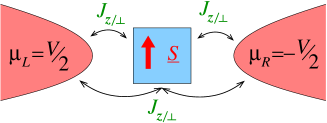
Figure 1: (Color online) A spin-$\frac{1}{2}$ quantum system coupled via exchange couplings $J_{z/\perp}$ to the spins of two reservoirs.

Method.—To study the dynamics of the local spin $\underline{S}(t)=\langle\underline{\hat{S}}\rangle(t)$ and the charge current $I(t)=\langle\hat{I}\rangle(t)$, we switch on the coupling $H_{ex}$ suddenly at the initial time $t=0$. It means that we prepare the initial density matrix in the product form $\rho(0)=\rho_{D}^{(0)}\rho_{L}\rho_{R}$, where $\rho_{D}^{(0)}$ is an arbitrary density matrix for the local spin, and $\rho_{L/R}$ are grand canonical distributions for the left and right reservoirs. For $t>0$, we calculate the dynamics from a kinetic equation for the reduced density matrix $\rho_{D}(t)=\text{Tr}_{res}\rho(t)$. Following Ref. RTRG-FS_1, , one obtains in Laplace space and in Liouvillian notation $\rho_{D}(z)=i/(z-L_{D}^{eff}(z))\,\rho^{(0)}_{D}$, where $L_{D}^{eff}(z)$ is an effective dot Liouvillian. The spin dynamics follows from $\underline{S}(t)=\text{Tr}_{D}\,\hat{\underline{S}}\,\rho_{D}(t)$, with $\rho_{D}(t)=\frac{1}{2\pi}\int dz\,e^{-izt}\rho_{D}(z)$. The current in Laplace space is given by $I(z)=-i\text{Tr}_{D}\Sigma_{I}(z)\rho_{D}(z)$, where $\Sigma_{I}(z)$ denotes the current kernel. $L_{D}^{eff}(z)$ and $\Sigma_{I}(z)$ have been calculated in Ref. RTRG-FS_2, for an arbitrary quantum dot in the Coulomb blockade regime with explicit formulas for the anisotropic Kondo model. The result is given by a systematic expansion in the dot-reservoir couplings from PMS cut off at scale $\Lambda_{z}=\max\{V,h_{0},|z|\}\gg T_{c}$. The PMS equations are well-known solyom_zawadowski_74 and given by $(d/d\Lambda)J_{z/\perp}(\Lambda)=-2J_{\perp}(\Lambda)\,J_{\perp/z}(\Lambda)/\Lambda$, with the solution

$$J_{z}(\Lambda)=c\,\frac{1+\left(\frac{T_{K}}{\Lambda}\right)^{4c}}{1-\left(\frac{T_{K}}{\Lambda}\right)^{4c}},\;J_{\perp}(\Lambda)=2c\,\frac{\left(\frac{T_{K}}{\Lambda}\right)^{2c}}{1-\left(\frac{T_{K}}{\Lambda}\right)^{4c}},$$ (3)

where $c^{2}=J_{z}^{2}-J_{\perp}^{2}$ and $T_{K}$ are two invariants. In the isotropic case one obtains $J_{z/\perp}(\Lambda)=1/(2\ln(\Lambda/T_{K}))$. For a study of the time dynamics it appears to be more convenient to expand in the couplings cut off at the time-dependent scale $\Lambda_{t}$ defined in (1). We have proven that this expansion is well-defined in the weak-coupling regime $\Lambda_{t}\gg T_{c}$ and equivalent to the expansion in $J(\Lambda_{z})$.

In conventional perturbation theory one approximates $L_{D}^{eff}(z)\approx L_{D}^{eff}(z=0)$ (Markov approximation) and considers only the terms up to second order in the bare exchange couplings $J_{z/\perp}^{(0)}$ (Born approximation). This approach fails to describe the current dynamics as well as yields simple exponential decay for the longitudinal (transverse) spin with the spin relaxation (decoherence) rate $\Gamma_{1}$ ($\Gamma_{2}$). In contrast, in this Letter we include non-Markovian terms and use a systematic perturbative approach in the renormalized couplings $J_{z/\perp}$. In particular, replacing the effective Liouvillian in the resolvent $1/(z-L_{D}^{eff}(z))$ by any of its nonzero eigenvalues $\lambda_{p}(z)$ evaluated up to $O(J^{2})$, we obtain an expression of the generic form

$$\tilde{Z}\biggl{[}z-\widetilde{\Delta}_{p}+{\sum_{b}}c_{b}J_{b}^{2}\,(z-z_{b})\ln\frac{\Lambda_{t}}{-i(z-z_{b})}\biggr{]}^{-1}.$$ (4)

The pole of this resolvent is denoted by $z_{p}=\lambda_{p}(z_{p})$. For the Kondo model, there are three nonzero poles ($p=1,\pm$) at $z_{1}=-i\Gamma_{1}$ and $z_{\pm}=\pm h-i\Gamma_{2}$, where $\Gamma_{1}=\pi J_{\perp}^{2}(h+\max\{V,h\})$ and $\Gamma_{2}=(\pi/2)J_{z}^{2}V+\Gamma_{1}/2$. The real parts of these poles up to $O(J)$ determine the quantities $\widetilde{\Delta}_{p}$, i.e. $\widetilde{\Delta}_{\pm}=\pm(1-J_{z}+J_{z}^{(0)})h_{0}$ and $\widetilde{\Delta}_{1}=0$. Besides the appearance of renormalized quantities, there are two new important contributions in (4). Firstly, the factor $\tilde{Z}=1-2(J_{z}-J_{z}^{(0)})$ occurs, which contains $J_{z}\equiv J_{z}(\Lambda_{t})$ and thereby determines the universal non-exponential short-time behavior. Secondly, the logarithmic part is also of non-Markovian form. It induces branch cuts in the complex plane with branch points $z_{b}$ located at $z_{b}=\pm h+nV-i\Gamma_{2}$ (for $p=1$) and $z_{b}=nV-i\Gamma_{1}$ or $z_{b}=\pm h+nV-i\Gamma_{2}$ (for $p=\pm$), with $n=0,\pm 1$ ($c_{b}$ and $J_{b}\equiv J_{z/\perp}$ are the certain coefficients and couplings). The branch cuts lead to exponential behavior on the scale $z_{b}$, not $z_{p}$, i.e. with oscillation frequencies involving the voltage as well as unexpected decay rates. These exponential terms are multiplied by additional power-law or logarithmic functions involving the scale $z_{b}-z_{p}$. Therefore, all logarithmic terms appearing in the long-time evolution are cut off by the difference of decay rates $\Gamma_{pp^{\prime}}=\Gamma_{p}-\Gamma_{p^{\prime}}$, a feature which is generic for all quantities entering the time evolution (cf. Ref. RTRG-FS_2, ).

Results.—Considering all poles and branch cuts of the resolvents (4) and closing the integration contour of the inverse Laplace transform in the lower half plane of $z$, we obtain after some lengthy algebra the following final result for the spin and current dynamics in closed form (we set $e=\hbar=1$ and assume $V,h>0$)

$$S_{z}(t) = S_{z}^{(0)}\,\tilde{Z}e^{-\Gamma_{1}t}+S_{z}^{st}(1-e^{-\Gamma_{1}t})-S_{z}^{(0)}J_{\perp}^{2}\,\text{Re}\!\left[S^{h+i\Gamma_{12}}_{z_{1}z_{+}}+S^{h-V+i\Gamma_{12}}_{z_{1},z_{+}-V}+(V\rightarrow-V)\right],$$ (5)

$$S_{+}(t) = S_{+}^{(0)}\,e^{-\Gamma_{2}t}e^{iht}\left[\tilde{Z}-J_{z}^{2}\ln(\Lambda_{t}t)\right]-\frac{1}{2}\,S_{+}^{(0)}\left[J_{z}^{2}S^{V}_{z_{-},z_{-}+V}+J_{\perp}^{2}(S^{h-i\Gamma_{12}}_{z_{-}z_{1}}+S^{h-V-i\Gamma_{12}}_{z_{-},z_{1}-V})+(V\rightarrow-V)\right],$$ (6)

$$I(t) = \frac{\pi}{4}(J_{z}^{2}+2J_{\perp}^{2})V+\pi J_{\perp}^{2}\min\{V,h\}S_{z}^{st}(1-e^{-\Gamma_{1}t})-\frac{1}{t}\,S_{z}^{(0)}J_{\perp}^{2}\,\text{Re}\!\left[I^{h-V+i\Gamma_{12}}_{z_{1},z_{+}-V}-(V\rightarrow-V)\right],$$ (7)

where $S_{+}=S_{x}+iS_{y}$ and $\Gamma_{12}=\Gamma_{1}-\Gamma_{2}$. The initial and the stationary magnetizations are denoted by $\underline{S}^{(0)}=\underline{S}(0)$ and $S_{z}^{st}=-h/(h+\max\{V,h\})$, and we have introduced the auxiliary functions $S^{\alpha}_{zz^{\prime}}(t)=e^{-izt}\ln\frac{\Lambda_{t}}{i\alpha}+e^{-iz^{\prime}t}F_{2}(\alpha t)$ and $I^{\alpha}_{zz^{\prime}}(t)=e^{-izt}i\alpha t\ln\frac{\Lambda_{t}}{i\alpha}+e^{-iz^{\prime}t}F_{1}(\alpha t)$, with $F_{k}(x)\!=\!(-1)^{k-1}\!\int_{0}^{\infty}dy\,ye^{-y}/(y+ix)^{k}$.

Equations (5)-(7) provide the time dynamics up to $O(J^{2})$ in all crossover regimes. We stress that all observables decay both with the relaxation and decoherence rates. Correction terms $\sim O(J^{2})$ oscillate with frequencies $h\pm V$, and, additionally, with $h$ ($nV;\,n=0,\pm$) for the longitudinal (transverse) spin. From an experimental point of view these oscillations along with the occurrence of both decay rates are our most important results. Examples for the time evolution in the isotropic case $J_{z}=J_{\perp}$ are shown in Figs. 2 and 3. We now illustrate the results in different time regimes.

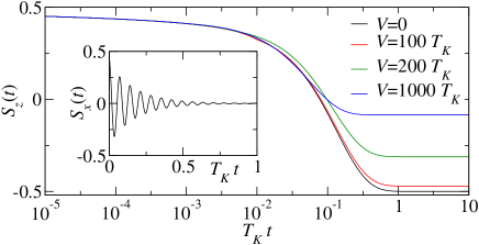
Figure 2: (Color online) $S_{z}(t)$ in the isotropic Kondo model for $h_{0}=100\,T_{K}$ and various values of the applied voltage $V$, with $S_{z}(0)=1/2$. Inset: $S_{x}(t)$ for $V=h_{0}=100\,T_{K}$ and $S_{x}(0)=1/2$, $S_{y}(0)=0$.

Long-time limit, off-resonance.—For large times $t\gg\max\{V,h_{0}\}^{-1}$, we have $\Lambda_{t}=\Lambda_{c}\equiv\max\{V,h_{0}\}$ and $J_{z/\perp}\equiv J_{z/\perp}(\Lambda_{c})$. In the off-resonance case $V,h,|h\pm V|\sim\Lambda_{c}$, we get typical power-law behavior from the asymptotic expansions $F_{1}(x)\approx-i/x$ and $F_{2}(x)\approx 1/x^{2}$, for $|x|\gg 1$. Besides the exponential decay, this gives additional factors $\sim 1/(\alpha t)^{k}$, with $k=1$ for the current and $k=2$ for the spin. For the transverse spin we obtain, for example,

$$S_{+}(t) \approx S_{+}^{(0)}e^{-\Gamma_{2}t}e^{iht}\left[Z-J_{z}^{2}\frac{\cos(Vt)}{V^{2}t^{2}}\right]$$

$$-S_{+}^{(0)}\frac{J_{\perp}^{2}}{2}e^{-\Gamma_{1}t}\left[\frac{2}{h^{2}t^{2}}+\frac{e^{iVt}}{(h-V)^{2}t^{2}}+\frac{e^{-iVt}}{(h+V)^{2}t^{2}}\right],$$

with $Z=\tilde{Z}-J_{z}^{2}\ln(\Lambda_{c}t)+i\frac{\pi}{2}\{J_{z}^{2}+J_{\perp}^{2}[2-\Theta(V-h)]\}$. To identify the different time scales from the exponential decay explicitly, situations where $\Gamma_{1}$ and $\Gamma_{2}$ differ significantly are of particular interest. For the anisotropic Kondo model at finite voltage this can be easily achieved since $\Gamma_{2}/\Gamma_{1}=1/2+O((J_{z}/J_{\perp})^{2})$. Thus, for $J_{z}\gg J_{\perp}$ we obtain $\Gamma_{2}\gg\Gamma_{1}$. This is typically the case for single molecular magnets, where the transverse exchange coupling is generated by quantum tunneling of magnetizationSMM_theory (e.g. in Fe₄ the ratio is $J^{(0)}_{\perp}/J^{(0)}_{z}\sim 10^{-5}$). Fig. 4 shows the clear separation of time scales for $S_{x}(t)$. The time scale at which the change of the leading behavior happens is approximately given by $t\sim 2|\ln J_{\perp}|/\Gamma_{21}$. At this time we also observe the change in the oscillation frequency from $h$ to $V$.

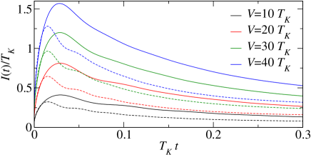
Figure 3: (Color online) Current $I(t)$ in the isotropic Kondo model for $h_{0}=100\,T_{K}$ (solid lines) and $h_{0}=200\,T_{K}$ (dashed lines) and various values of the applied voltage $V$, with $S_{z}(0)=1/2$. We observe oscillations at times $T_{K}t\sim 0.05$; the stationary current is reached for $T_{K}t\geq 0.5$.

Long-time limit, on-resonance.—For large times $t\gg\Lambda_{c}^{-1}$ and close to resonances, where $|\delta|\ll\Lambda_{c}$, with $\delta=h-V$ or $\delta=h$, we can enter the interesting time regime $|\delta t|\ll 1$. In this case, we obtain logarithmic contributions from $F_{k}(\alpha t)$, with $|\alpha t|\ll 1$ and $\alpha=\delta-i\Gamma_{12}$. For the longitudinal spin and the current, the logarithmic terms $\sim\ln|\delta t|$ cancel out. In turn, for the transverse spin we obtain the logarithmic contributions

$$S_{+}(t)\rightarrow-a\,e^{i\pi/2}\,S_{+}^{(0)}\,J_{\perp}^{2}\,\delta t\ln|(\delta-i\Gamma_{12})t|,$$ (9)

with $a=1/2,1$ for $\delta=h-V,h$. As a consequence, the spin perpendicular to the plane defined by the $z-$axis and the initial direction obtains a logarithmic enhancement at resonance $\delta\rightarrow 0$ after taking the derivative $\frac{d}{d\delta}$. The cutoff of the logarithm at $\delta=0$ is determined by the difference $\Gamma_{12}$ of the rates. Especially for $\delta=h\ll V$ in the isotropic model the cutoff scale $\Gamma_{12}=\frac{\pi}{2}J^{2}h$ becomes zero close to resonance. In this case the perturbative approach breaks down for exponentially small values of $ht$ where $J\ln|ht|\sim O(1)$. This regime is beyond our approach and requires a nonperturbative treatment.

Short-time limit.—For short timesultra_short $D^{-1}\ll t\ll\Lambda_{c}^{-1}$ we get $\Lambda_{t}=1/t$ and $J_{z/\perp}\equiv J_{z/\perp}(1/t)\equiv J_{z/\perp}^{t}$. The terms containing $(S/I)^{\alpha}_{zz^{\prime}}$ are negligible and we obtain from the first terms of (5)-(7) the universal result

$$\underline{S}(t) = \tilde{Z}\,\underline{S}^{(0)}\,=\,(1-2J_{z}^{t}+2J_{z}^{(0)})\,\underline{S}^{(0)},$$ (10)

$$G(t) = \frac{I(t)}{V}\,=\,\frac{e^{2}}{h}\frac{\pi^{2}}{2}\left[(J_{z}^{t})^{2}+2(J_{\perp}^{t})^{2}\right].$$ (11)

For $J_{z}^{(0)}\gg J_{\perp}^{(0)}$ and $|(T_{K}t)^{4c}|\ll 1$ (AFM case), we get

$$\underline{S}(t) = \underline{S}(0)\{1+2J_{z}^{(0)}-2c-4c(T_{K}t)^{4c}\},$$ (12)

$$G(t) = \frac{e^{2}}{h}\left[\frac{\pi^{2}}{2}c^{2}\,+\,6\pi^{2}c^{2}(T_{K}t)^{4c}\right],$$ (13)

with $c=\sqrt{(J_{z}^{(0)})^{2}-(J_{\perp}^{(0)})^{2}}$. For $|(T_{K}t)^{4c}|\gg 1$ (FM case), we have to replace $c\rightarrow-c$. As a result, universal power laws are predicted in the short-time limit on the scale of the Kondo temperature. We note that for the FM Kondo model with $V=h_{0}=0$ a power law has also been found for $S_{z}(t)$ in Ref. Hackl_etal_09, . Here, we have found a complete analytic expression in terms of the PMS solution, together with results for the AFM model, the transverse spin, and the current. Furthermore, we identified the validity range for finite $\Lambda_{c}$ by $t\ll\Lambda_{c}^{-1}$. In the isotropic case ($c=0$), we obtain $J^{t}=-1/(2\ln(T_{K}t))$ leading to $\underline{S}(t)=\underline{S}(0)(1+2J_{z}^{(0)}+1/\ln(T_{K}t))$ and $G(t)=(e^{2}/h)3\pi^{2}/(8\ln^{2}(T_{K}t))$ for both AFM and FM models. In this case, universal logarithmic terms occur, which have also been found for $S_{z}(t)$ in Refs. Roosen_etal_08, ; Hackl_etal_09, .

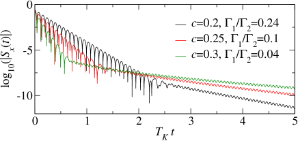
Figure 4: (Color online) $\log_{10}(|S_{x}(t)|)$ in the anisotropic Kondo model for $V=2h_{0}=100\,T_{K}$ and various values of the anisotropy $c^{2}=(J_{z}^{(0)})^{2}-(J_{\perp}^{(0)})^{2}$, with $S_{x}(0)=1/2$, $S_{y}(0)=0$. The dips have their origin in the oscillations of $S_{x}(t)$.

Summary.—We found complex dynamics for a spin coupled to fermionic reservoirs held at finite bias and for the current across it. The results go beyond Markovian theories and, in a well-controlled weak-coupling regime, are presented in closed analytic form covering all time regimes. Due to the generic form of Eq.(4), we propose our main conclusions to be generic for quantum dots in the Coulomb blockade regime. From Ref. RTRG-FS_2, it follows that the branch points of the logarithmic terms are generically given by $z_{b}=z_{p}+nV$, where $z_{p}$ is any pole of the leading order exponential decay, and $n=0,\pm 1,\pm 2,\dots$. Therefore, we find in all orders of perturbation theory that all terms are exponentially decaying, all transport rates occur in principle in the decay of each observable, and the voltage appears in the oscillation frequencies. We have shown this explicitly for the Kondo model and revealed that the bias voltage is an important energy scale for the time evolution showing up in unexpected oscillation frequencies and in various power-law and logarithmic contributions.

This work was supported by the DFG-FG 723 and 912.

References

(1)
P. F. Braun et al., Phys. Rev. Lett. 94, 116601 (2005);
K. C. Nowack et al., Science 318, 1430 (2007);
M. Atatüre et al., Nat. Phys. 3, 101 (2007).
(2)
J. Preskill, in Introduction to Quantum Computation and Information
(H.-K. Lo, S. Popescu, and T. Spiller, World Scientific, Singapore, 1998)
p. 213;
D. P. Di Vincenzo and D. Loss, Phys. Rev. B 71, 035318 (2005);
J. Fischer and D. Loss, Science 324, 1277 (2009).
(3)
F. B. Anders and A. Schiller, Phys. Rev. Lett. 95, 196801 (2005);
ibid., Phys. Rev. B 74, 245113 (2006);
F. B. Anders, R. Bulla, and M. Vojta, Phys. Rev. Lett. 98, 210402 (2007).
(4)
D. Roosen, M. R. Wegewijs, and W. Hofstetter,
Phys. Rev. Lett. 100, 087201 (2008).
(5)
A. Daley et al., J. Stat. Mech.: Theor. Exp. P04005 (2004);
S. R. White and A. Feiguin, Phys. Rev. Lett. 93, 076401 (2004);
P. Schmitteckert, Phys. Rev. B 70, 121302 (2004);
F. Heidrich-Meisner, A. E. Feiguin, and E. Dagotto,
Phys. Rev. B 79, 235336 (2009).
(6)
S. Weiss et al., Phys. Rev. B 77, 195316 (2008).
(7)
T. L. Schmidt et al., Phys. Rev. B 78, 235110 (2008).
(8)
F. Lesage and H. Saleur, Phys. Rev. Lett. 80, 4370 (1998);
A. Schiller and S. Hershfield, Phys. Rev. B 62, R16271 (2000);
A. Komnik, Phys. Rev. B 79, 245102 (2009).
(9)
H. Schoeller, Eur. Phys. J. Special Topics 168, 179 (2009).
(10)
H. Schoeller, in Low-Dimensional Systems
(ed. T. Brandes, Lect. Notes Phys. Vol. 544, Springer, 2000) p. 137;
H. Schoeller and J. König, Phys. Rev. Lett. 84, 3686 (2000);
S. G. Jakobs, V. Meden, and H. Schoeller,
Phys. Rev. Lett. 99, 150603 (2007).
(11)
A. Rosch et al., Phys. Rev. Lett. 90, 076804 (2003);
ibid., J. Phys. Soc. Jpn. 74, 118 (2005).
(12)
S. Kehrein, Phys. Rev. Lett. 95, 056602 (2005).
(13)
A. Hackl and S. Kehrein, Phys. Rev. B 78, 092303 (2008).
(14)
H. Schoeller and F. Reininghaus, Phys. Rev. B 80, 045117 (2009);
ibid. Phys. Rev. B 80, 209901(E) (2009).
(15)
D. Schuricht and H. Schoeller, Phys. Rev. B 80, 075120 (2009).
(16)
M. Keil and H. Schoeller, Phys. Rev. B 63, 180302(R) (2001).
(17)
A. Hackl et al., Phys. Rev. Lett. 102, 219902 (2009);
A. Hackl, M. Vojta, and S. Kehrein, Phys. Rev. B 80, 195117 (2009).
(18)
D. Lobaskin and S. Kehrein, Phys. Rev. B 71, 193303 (2005).
(19)
L. I. Glazman and M. Pustilnik, in Nanophysics: Coherence and Transport
(H. Bouchiat et al., Elsevier, 2005) p. 427.
(20)
D. Goldhaber-Gordon et al., Nature (London) 391, 156 (1998);
S. M. Cronenwett, T. H. Oosterkamp, and L. P. Kouwenhoven,
Science 281, 540 (1998).
(21)
C. Romeike et al., Phys. Rev. Lett. 96, 196601 (2006);
H. B. Heersche et al., Phys. Rev. Lett. 96, 206801 (2006);
M.-H. Jo et al., Nano Lett. 6, 2014 (2006).
(22)
We assume the exchange couplings to be independent of the
reservoir index. Other cases can be equally well treated.
(23)
J. Solyom and A. Zawadowski, J. Phys. F: Metal Phys. 4, 80 (1974).
(24) At ultra-short times an expansion in
and is applicable. The scale is
invisible in this regime.