Dynamics of a two-species Bose-Einstein condensate in a double well

Abstract

We study the dynamics of a two-species Bose-Einstein condensate in a double well. Such a system is characterized by the intra-species and inter-species $s$-wave scattering as well as the Josephson tunnelling between the two wells and the population transfer between the two species. We investigate the dynamics for some interesting regimes and present numerical results to support our conclusions. In the case of vanishing intra-species scattering lengths and a weak inter-species scattering length, we find collapses and revivals in the population dynamics. A possible experimental implementation of our proposal is briefly discussed.

I introduction

Soon after the realization of scalar Bose-Einstein condensates (BECs) in laboratories, there has been great interest in exploring two species BECs both experimentally wieman ; cornell0 ; cornell ; ketterle0 ; ketterle ; cornell2 ; holland ; ingu0 ; ingu1 ; grimm ; ingu2 ; wieman2 and theoretically ho ; eberly ; bigelow ; bigelow2 ; graham ; ricardo ; carr ; bohn ; ricardo2 . Such a two species BEC provides an ideal platform for the study of more intriguing phenomena. It can help us understand some basic problems in ultralow temperature physics like interpenetrating ³He-⁴He mixtures. The two species can be two alkali like ²³Na-⁸⁷Rb or two isotopes like ⁸⁵Rb-⁸⁷Rb. It can also be two hyperfine states of the same alkali. Different from the case of a scalar condensate, we need three scattering lengths to characterize the $s$-wave scattering between alike and unlike atoms, which is referred to as intra-species and inter-species scattering, respectively. The interplay between the inter-species and intra-species scattering has a direct consequence on the properties of the condensates, e.g. the density profile ho ; bigelow and collective excitations bigelow2 . For example, as shown in a pioneering work by Ho and Shenoy ho , the phase of trapped condensates can smoothly evolve from interpenetrating to separate by changing the atom numbers and/or the scattering lengths.

In addition to studying the stationary properties of BECs, the coherent dynamics of a two species BEC can be investigated by propagating coupled Gross-Pitaevskii equations. Previous work has shown various interesting dynamics for two-species BECs zhang ; liu1 ; liu2 ; ricardo2 . For this paper, we focus on the case of the two species being two hyperfine states of the same alkali. One can manipulate such a two species BEC either by turning on the population transfer between the two internal states using a coupling microwave field savage ; hollanda ; kuang ; liu ; you ; xie or by placing it in a double well to allow for Josephson tunnelling law ; liang ; yang ; weiss ; clark . For the latter case, the double well is fundamental to the study of the Josephson effect in BECs. Smerzi and co-workers have shown that a scalar BEC trapped in a double well exhibits rich dynamics such as Rabi oscillations and macroscopic quantum self-trapping smerzi ; smerzi2 ; smerzi3 . It has also been shown that there exists non-Abelian Josephson effect between two $F=2$ spinor BECs in double optical traps liu3 . Therefore it is of great interest to study the behavior of a two species BEC in a double well. Previous work on a two species BEC has focused either on the population transfer or on Josephson tunnelling. To the best of our knowledge, the combination of both of them has not been addressed in the literature. It is the purpose of this paper to discuss some interesting phenomena involving both population transfer and Josephson tunnelling.

This paper is organized as follows. In Sec. II, we first introduce our model Hamiltonian and various parameters. In Sec. III, we then discuss some interesting regimes and give our numerical results. We summarize our findings in Sec. IV. Finally, an appendix is given in Sec. V.

II model

In this paper, we consider a two species Bose-Einstein condensate in a double well. We focus on the case where the two species are for two different hyperfine spin states, e.g. ⁸⁷Rb condensates in $|1\rangle\equiv|F=1,m_{F}=-1\rangle$ and $|2\rangle\equiv|F=2,m_{F}=1\rangle$, and they are subjected to the same trapping potential. We adopt the well-known two-mode approximation, i.e. $\Psi_{\alpha,j}({\bf r})\simeq a_{\alpha,j}\psi_{\alpha}({\bf r})$. The Greek letter $\alpha=L(R)$ denotes the left (right) well and the Roman letter $j=1(2)$ labels the two species. $\psi_{\alpha}({\bf r})$ is the ground state solution of the $\alpha$ well which is independent of the species. $a_{\alpha,j}$ is the annihilation operator for species $i$ in the $\alpha$ well, satisfying $[a_{\alpha,j},a_{\beta,k}^{\dagger}]=\delta_{\alpha,\beta}\delta_{j,k}$. Here $\delta_{p,q}$ is the Kronecker delta. In the second quantization formalism, the Hamiltonian is ($\hbar=1$)

$$H = \sum_{\alpha=L,R;j=1,2}\epsilon_{\alpha}a_{\alpha,j}^{\dagger}a_{\alpha,j}+J\sum_{j}(a_{L,j}^{\dagger}a_{R,j}+a_{L,j}a_{R,j}^{\dagger})$$ (1)

$$+ \sum_{\alpha}\left[{g_{11}^{(\alpha)}\over 2}a_{\alpha,1}^{\dagger}a_{\alpha,1}^{\dagger}a_{\alpha,1}a_{\alpha,1}+{g_{22}^{(\alpha)}\over 2}a_{\alpha,2}^{\dagger}a_{\alpha,2}^{\dagger}a_{\alpha,2}a_{\alpha,2}\right.$$

$$+ \left.g_{12}^{(\alpha)}a_{\alpha,1}^{\dagger}a_{\alpha,2}^{\dagger}a_{\alpha,1}a_{\alpha,2}+\Omega(a_{\alpha,1}^{\dagger}a_{\alpha,2}+a_{\alpha,1}a_{\alpha,2}^{\dagger})\right].$$

$\epsilon_{\alpha}$ is the single particle energy in the $\alpha$ well. $2J=\int d{\bf r}\psi_{L}^{*}({\bf r})(T+V({\bf r}))\psi_{R}({\bf r})+\int d{\bf r}\psi_{L}({\bf r})(T+V({\bf r}))\psi_{R}^{*}({\bf r})$ is the intra-species Josephson tunnelling rate between the left and right well which is referred to as tunnelling in the following. Here $T$ and $V$ are the kinetic and potential (double well) operator of a single particle, respectively. $J$ can be tuned by changing the shape of the double well. $g_{ij}^{(\alpha)}\equiv(4\pi\hbar^{2}a_{ij}/m)\int d{\bf r}|\psi_{\alpha}({\bf r})|^{4}$ is the interaction strength between species $i$ and $j$ in the $\alpha$ well. $a_{ij}$ is the $s$-wave scattering length between species $i$ and $j$. In this study, we only consider the case of repulsive interactions, i.e. $a_{ij}>0$. $m$ is the atom mass. $2\Omega$ is the Rabi frequency for the inter-species population transfer which is referred to as coupling in the following. It is proportional to the amplitude of the microwave field which resonantly couples the two internal states. For simplicity, we assume $J\geq 0$ and $\Omega\geq 0$. In addition, we consider a symmetric double well in this paper, thus $\epsilon_{L}=\epsilon_{R}$ and $\psi_{L}({\bf r})=\psi_{R}({\bf r})$. Correspondingly, $g_{ij}^{(L)}=g_{ij}^{(R)}$ and the superscript is then dropped afterwards. A schematic view of our model system is shown in Fig. 1. We note that the Hamiltonian of Eq. (1) resembles the cross phase modulation between two modes of light in a nonlinear Kerr medium. The terms involving $\Omega$ and $J$ are analogous to the Hamiltonian of a beam splitter. In the point view of quantum optics, our Hamiltonian describes the combination of nonlinear beam splitters.

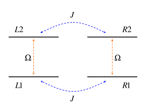
Figure 1: (Color online) A schematic view of our model system where the solid lines represent the four modes and the dashed lines represents the coupling (red) and tunnelling (blue). The $s$-wave scattering terms are not shown in this figure.

We assume that initially all $N$ atoms are of species 1 and localized in the left well, i.e. $|\psi(t=0)\rangle\propto(a_{L,1}^{\dagger})^{N}|\rm vac\rangle$. The coupling $\Omega$ and $J$ are turned on at $t=0$ and we investigate the subsequent dynamics.

III various regimes

We categorize our model into three regimes: the strong coupling/tunnelling regime $(\Omega,J)\gg g_{ij}(N-1)$, the strong interaction regime $g_{ij}(N-1)\gg(\Omega,J)$, and the intermediate regime where the terms of $g_{ij}(N-1)$, $\Omega$, and $J$ have equally important contributions to the dynamics. In the following, we will discuss these three regimes separately.

We first consider the strong coupling/tunnelling regime so the collisional interaction terms are neglected. The Hamiltonian is

$$H_{C}^{(o)} = \Omega(a_{L,1}^{\dagger}a_{L,2}+a_{R,1}^{\dagger}a_{R,2}+a_{L,1}a_{L,2}^{\dagger}+a_{R,1}a_{R,2}^{\dagger})$$

$$+ J(a_{L,1}^{\dagger}a_{R,1}+a_{L,2}^{\dagger}a_{R,2}+a_{L,1}a_{R,1}^{\dagger}+a_{L,2}a_{R,2}^{\dagger}).$$

It is easy to verify that the terms in the bracket involving $\Omega$ commute with those involving $J$. $H_{C}^{(o)}$ can be written in a more compact form $H_{C}^{(o)}={\bf a}^{\dagger}\cdot{\bf M}\cdot{\bf a}$ where ${\bf a}=(a_{L,1},a_{L,2},a_{R,1},a_{R,2})^{\rm T}$. The matrix ${\bf M}$ depends only on $\Omega$ and $J$. This Hamiltonian is quadratic, so it can be simplified in a standard manner by diagonalizing ${\bf M}$. Explicitly, by the following transformation,

$$f_{1} = {1\over 2}(a_{L,1}+a_{L,2}+a_{R,1}+a_{R,2}),$$

$$f_{2} = {1\over 2}(a_{L,1}-a_{L,2}-a_{R,1}+a_{R,2}),$$

$$g_{1} = {1\over 2}(a_{L,1}+a_{L,2}-a_{R,1}-a_{R,2}),$$

$$g_{2} = {1\over 2}(a_{L,1}-a_{L,2}+a_{R,1}-a_{R,2}).$$ (3)

$[f_{j},f_{k}^{\dagger}]=\delta_{jk}$ and $[g_{j},g_{k}^{\dagger}]=\delta_{jk}$ with all other commutators being zero. The conservation of atom numbers leads to $f_{1}^{\dagger}f_{1}+f_{2}^{\dagger}f_{2}+g_{1}^{\dagger}g_{1}+g_{2}^{\dagger}g_{2}=N$. The Hamiltonian can be rewritten in the form of new operators

$$H_{C}=(\Omega+J)(f_{1}^{\dagger}f_{1}-f_{2}^{\dagger}f_{2})+(\Omega-J)(g_{1}^{\dagger}g_{1}-g_{2}^{\dagger}g_{2}),$$ (4)

where constant terms have been dropped out. We note that the net effect of coupling and tunnelling can be either constructive ($\Omega+J$) where the coupling and tunnelling are in phase or destructive ($\Omega-J$) where they are out of phase, analogous to the center of mass and the relative motion of two particles, respectively. The corresponding initial condition is $|\psi(t=0)\rangle\propto[f_{1}^{\dagger}+f_{2}^{\dagger}+g_{1}^{\dagger}+g_{2}^{\dagger}]^{N}|\rm vac\rangle$.

The wave function at any time $t$ can be obtained with the help of the following identity

$$e^{-iH_{C}t}(f_{1}^{\dagger}+f_{2}^{\dagger}+g_{1}^{\dagger}+g_{2}^{\dagger})e^{iH_{C}t}$$

$$= e^{-i(\Omega+J)t}f_{1}^{\dagger}+e^{i(\Omega+J)t}f_{2}^{\dagger}+e^{-i(\Omega-J)t}g_{1}^{\dagger}+e^{i(\Omega-J)t}g_{2}^{\dagger}.$$

Therefore,

$$|\psi(t)\rangle={1\over 2^{N}\sqrt{N!}}\left[e^{-i(\Omega+J)t}f_{1}^{\dagger}+e^{i(\Omega+J)t}f_{2}^{\dagger}\right.$$

$$\left.+e^{-i(\Omega-J)t}g_{1}^{\dagger}+e^{i(\Omega-J)t}g_{2}^{\dagger}\right]^{N}|\rm vac\rangle.$$

Substituting $a_{\alpha,j}^{\dagger}$ back into the above expression, we obtain the normalized wave function

$$|\psi(t)\rangle = {1\over\sqrt{N!}}\left[\sum_{\alpha=L,R;j=1,2}S_{\alpha,j}(t)a_{\alpha,j}^{\dagger}\right]^{N}|\rm vac\rangle,$$

$$S_{L,1}(t) = {{\rm cos}(\Omega+J)t+{\rm cos}(\Omega-J)t\over 2},$$

$$S_{R,2}(t) = {{\rm cos}(\Omega+J)t-{\rm cos}(\Omega-J)t\over 2},$$

$$S_{L,2}(t) = -i{{\rm sin}(\Omega+J)t+{\rm sin}(\Omega-J)t\over 2},$$

$$S_{R,1}(t) = -i{{\rm sin}(\Omega+J)t-{\rm sin}(\Omega-J)t\over 2}.$$ (5)

Various quantities can be calculated directly from the wave function. For instance, the first order coherence between modes $a_{\alpha,j}$ and $a_{\beta,k}$ is found to be

$$g^{(1)}_{\alpha,j;\beta,k}(t) = {1\over N}\langle\psi(t)|a_{\alpha,j}^{\dagger}a_{\beta,k}|\psi(t)\rangle$$ (6)

$$= S^{*}_{\alpha,j}(t)S_{\beta,k}(t).$$

Especially, the fraction of species $j$ in the $\alpha$ well is given by

$$n_{\alpha,j}(t)=g^{(1)}_{\alpha,j;\alpha,j}(t)=|S_{\alpha,j}(t)|^{2}.$$ (7)

Higher order coherence terms can be derived straightforwardly with similar patterns and will not be presented here. We note that at any time $t>0$, there is a balancing condition $n_{L1}/n_{L2}=n_{R1}/n_{R2}$ for the given initial state.

Our conclusion also applies to the case with temporal modulations of $\Omega$ and $J$ if we make the replacement

$$e^{-iH_{C}t}\to e^{-i\int_{0}^{t}H_{C}(t^{\prime})dt^{\prime}}.$$ (8)

The time ordered exponential is not needed here since the hamiltonian commutes at any time in this representation. Therefore, the effect of time dependence is determined from two pulse areas, i.e. $\int_{0}^{t}(\Omega(t^{\prime})+J(t^{\prime}))dt^{\prime}$ and $\int_{0}^{t}(\Omega(t^{\prime})-J(t^{\prime}))dt^{\prime}$. If we assume a form of $\Omega(t^{\prime})=\Omega_{0}e^{-t^{\prime}/\tau}$ and $J=J_{0}e^{-t^{\prime}/\tau}$, then the two pulse areas are $(\Omega_{0}+J_{0})\tau(1-e^{-t/\tau})$ and $(\Omega_{0}-J_{0})\tau(1-e^{-t/\tau})$ for the case of in phase and out of phase, respectively. For a long enough time $t\gg\tau$, the exponential terms in the above pulse areas can be neglected and the tunnelling dynamics are suppressed. The wave function takes the same form as Eq. 5 except for the replacements $\Omega\to\Omega_{0},J\to J_{0},$ and $t\to\tau$. A numerical example is shown in Fig. 2. Unless otherwise specified, the energy and time scale are $\omega_{0}$ and $1/\omega_{0}$, respectively, where $\omega_{0}$ is the angular frequency obtained by approximating one well as harmonic.

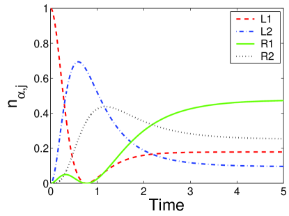
Figure 2: (Color online) Fraction of each component as a function of time. $\Omega=3.2,J=1.3,\tau=\pi/4,g_{11}=g_{22}=g_{12}=0$.

In the opposite regime where the nonlinear interaction dominates, the coupling between the two species is still on resonance. However, the tunnelling between the left and right well is frozen due to the large detuning. For instance, the energy difference between the two Fock states $|N\rangle_{L1}|0\rangle_{L2}|0\rangle_{R1}|0\rangle_{R2}$ and $|N-1\rangle_{L1}|0\rangle_{L2}|1\rangle_{R1}|0\rangle_{R2}$ is $\propto g_{11}(N-1)\gg J$ for large $N$. So the dynamics are restricted to the left well which is essentially a two-level system. A numerical example is shown in Fig. 3 where we can clearly see that the dynamics are restricted to the two species in the left well and the tunnelling to the right well is suppressed.

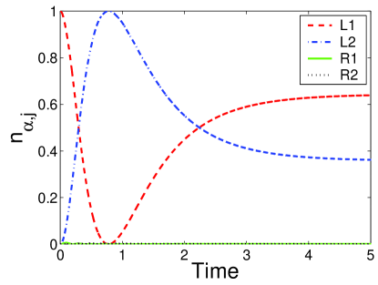
Figure 3: (Color online) Fraction of each component as a function of time. $\Omega=3.2,J=1.3,\tau=\pi/4,g_{11}=g_{22}=g_{12}=35$.

In the intermediate regime, we cannot obtain solutions in closed form in general. In the following, we will consider a specific case where we can obtain some analytical results. We assume $g_{11}=g_{22}=0$ and the term involving $g_{12}$ is a perturbation to the coupling/tunnelling. We denote $g_{12}=g$ in the following. Motivated by the strong coupling/tunnelling case, we adopt the following transformation

$$a_{L,1}={1\over 2}[e^{i\omega_{+}t}f_{1}+e^{-i\omega_{+}t}f_{2}+e^{i\omega_{-}t}g_{1}+e^{-i\omega_{-}t}g_{2}],$$

$$a_{L,2}={1\over 2}[e^{i\omega_{+}t}f_{1}-e^{-i\omega_{+}t}f_{2}+e^{i\omega_{-}t}g_{1}-e^{-i\omega_{-}t}g_{2}],$$

$$a_{R,1}={1\over 2}[e^{i\omega_{+}t}f_{1}-e^{-i\omega_{+}t}f_{2}-e^{i\omega_{-}t}g_{1}+e^{-i\omega_{-}t}g_{2}],$$

$$a_{R,2}={1\over 2}[e^{i\omega_{+}t}f_{1}+e^{-i\omega_{+}t}f_{2}-e^{i\omega_{-}t}g_{1}-e^{-i\omega_{-}t}g_{2}],$$ (9)

where $\omega_{\pm}\equiv 2(\Omega\pm J)$. $f_{j}$ and $g_{j}$ obey the same commutation conditions as in the strong coupling/tunnelling case. Substituting $a_{\alpha,j}$ into the Hamiltonian (1), we then invoke the rotating wave approximation (RWA) to eliminate the fast oscillating terms and only keep resonant terms. Explicitly, RWA requires $g\ll(\Omega,J,|\Omega-J|,|2\Omega-J|,|\Omega-2J|)$. The new Hamiltonian becomes

$$H_{R} = {g\over 8}\left(f_{1}^{\dagger}f_{1}^{\dagger}f_{1}f_{1}+f_{2}^{\dagger}f_{2}^{\dagger}f_{2}f_{2}+g_{1}^{\dagger}g_{1}^{\dagger}g_{1}g_{1}\right.$$ (10)

$$\left.+g_{2}^{\dagger}g_{2}^{\dagger}g_{2}g_{2}+4f_{1}^{\dagger}g_{1}^{\dagger}f_{1}g_{1}+4f_{2}^{\dagger}g_{2}^{\dagger}f_{2}g_{2}\right)$$

$$+(\Omega+J)(f_{1}^{\dagger}f_{1}-f_{2}^{\dagger}f_{2})$$

$$+(\Omega-J)(g_{1}^{\dagger}g_{1}-g_{2}^{\dagger}g_{2}).$$

This Hamiltonian is separable in two groups of modes $(f_{1},g_{1})$ and $(f_{2},g_{2})$. Each group of modes, $f_{j}$ and $g_{j}$, are coupled by the mean field interaction and the detuning between them is $2J$. The above Hamiltonian is already diagonal in the basis of $f_{j}$ and $g_{j}$, so we label the Fock eigenstate as $|mnpq)$ in the basis order of $f_{1},f_{2},g_{1},g_{2}$. The corresponding energy is $E_{mnpq}=E_{m,p}+E_{n,q}$ with

$$E_{m,p} = {g\over 8}(m^{2}-m+p^{2}-p+4mp)$$

$$+(\Omega+J)m+(\Omega-J)p,$$

$$E_{n,q} = {g\over 8}(n^{2}-n+q^{2}-q+4nq)$$

$$-(\Omega+J)n-(\Omega-J)q.$$

Note that as $|\rm vac\rangle=|\rm vac)$, the wave function can be computed in the new basis as

$$|\psi(t)\rangle$$

$$= e^{-iH_{R}t}{1\over 2^{N}\sqrt{N!}}(f_{1}^{\dagger}+f_{2}^{\dagger}+g_{1}^{\dagger}+g_{2}^{\dagger})^{N}|\rm vac\rangle$$

$$= e^{-iH_{R}t}{1\over 2^{N}}\sum_{mnpq}\delta_{N,m+n+p+q}{\sqrt{N!}\over\sqrt{m!n!p!q!}}|mnpq)$$

$$= {1\over 2^{N}}\sum_{mnpq}\delta_{N,m+n+p+q}{\sqrt{N!}\over\sqrt{m!n!p!q!}}e^{-iE_{mnpq}t}|mnpq).$$

The fraction of each species $n_{\alpha,j}$ can be computed with the help of the following results where the average is taken with respect to the wave function $|\psi(t)\rangle$:

$$\langle f_{1}^{\dagger}f_{1}\rangle = \langle f_{2}^{\dagger}f_{2}\rangle=\langle g_{1}^{\dagger}g_{1}\rangle=\langle g_{2}^{\dagger}g_{2}\rangle={N\over 4},$$

$$\langle f_{1}^{\dagger}f_{2}\rangle = e^{2i(\Omega+J)t}{N\over 4}\left({\cos(tg/4)+\cos(tg/2)\over 2}\right)^{N-1},$$

$$\langle f_{1}^{\dagger}g_{1}\rangle = e^{2iJt}{N\over 4}\left({1+\cos(tg/4)\over 2}\right)^{N-1},$$

$$\langle f_{1}^{\dagger}g_{2}\rangle = e^{2i\Omega t}{N\over 4}\left({\cos(tg/4)+\cos(tg/2)\over 2}\right)^{N-1},$$

$$\langle f_{2}^{\dagger}g_{1}\rangle = e^{-2i\Omega t}{N\over 4}\left({\cos(tg/4)+\cos(tg/2)\over 2}\right)^{N-1},$$

$$\langle f_{2}^{\dagger}g_{2}\rangle = e^{-2iJt}{N\over 4}\left({1+\cos(tg/4)\over 2}\right)^{N-1},$$

$$\langle g_{1}^{\dagger}g_{2}\rangle = e^{2i(\Omega-J)t}{N\over 4}\left({\cos(tg/4)+\cos(tg/2)\over 2}\right)^{N-1}.$$

In the Appendix, we give a derivation of $\langle f_{1}^{\dagger}f_{2}\rangle$. Other average values can be derived along similar lines.

After some algebra, we obtain

$$n_{L,1}={1\over 4}\left[1+\cos(2Jt)\left({1+\cos(tg/4)\over 2}\right)^{N-1}\right.$$

$$\left.+\cos(2\Omega t)(1+\cos(2Jt))\left({\cos(tg/4)+\cos(tg/2)\over 2}\right)^{N-1}\right],$$

(13)

$$n_{L,2}={1\over 4}\left[1+\cos(2Jt)\left({1+\cos(tg/4)\over 2}\right)^{N-1}\right.$$

$$\left.-\cos(2\Omega t)(1+\cos(2Jt))\left({\cos(tg/4)+\cos(tg/2)\over 2}\right)^{N-1}\right],$$

(14)

$$n_{R,1}={1\over 4}\left[1-\cos(2Jt)\left({1+\cos(tg/4)\over 2}\right)^{N-1}\right.$$

$$\left.+\cos(2\Omega t)(1-\cos(2Jt))\left({\cos(tg/4)+\cos(tg/2)\over 2}\right)^{N-1}\right],$$

(15)

$$n_{R,2}={1\over 4}\left[1-\cos(2Jt)\left({1+\cos((tg/4))\over 2}\right)^{N-1}\right.$$

$$\left.-\cos(2\Omega t)(1-\cos(2Jt))\left({\cos(tg/4)+\cos(tg/2)\over 2}\right)^{N-1}\right].$$

(16)

Therefore, in the case of the vanishing intra-species scattering, $n_{\alpha,j}$ will be subjected to collapses and revivals (CR). CR is a quantum mechanical effect which is well known in quantum optics. It is also found for a scalar BEC wall as well as for a two-species condensate in a single well kuang . The nonlinearity $g$ determines the envelope of the revivals as well as the time separation between the adjacent collapse and revival. It is easy to show that the width of the revival in the time domain is $\propto 1/(g\sqrt{N-1})$ for $N>1$ and the separation between a neighboring CR is $8\pi/g$. The coupling $\Omega$ and tunnelling $J$ determine the detailed structures of the oscillation inside the revival envelopes. Here we want to point out a major difference between our study and that of a two species BEC in a single well. In our case, CR is not observed for general scattering lengths $a_{ij}$. When the intra-species scattering lengths are not negligible, the population dynamics usually display quite complicated temporal patterns. We note that, for large $N$, since $n_{\alpha,j}$ are all small except for $gt/4=2n\pi$, we have

$${1+\cos(tg/4)\over 2}\sim e^{-\sin^{2}(tg/8)},$$

$${\cos(tg/4)+\cos(tg/2)\over 2}\sim e^{-5\sin^{2}(tg/8)}.$$ (17)

So up to some factors, our expressions take the same exponential form as those in Ref. kuang , e.g. Eq. (31). This is expected because the relative difference between a coherent state and a Fock state is small for large (average) atom numbers. We also note that, for $N=1$, $n_{\alpha,j}$ reduces to the results of the strong coupling/tunnelling regime.

The population difference between the two wells/species takes a relatively simpler form which is shown below

$$D_{LR} \equiv (n_{L,1}+n_{L,2})-(n_{R,1}+n_{R,1})$$

$$= \cos(2Jt)\left({1+\cos(tg/4)\over 2}\right)^{N-1},$$

$$D_{12} \equiv (n_{L,1}+n_{R,1})-(n_{L,2}+n_{R,2})$$ (18)

$$= \cos(2\Omega t)\left({\cos(tg/4)+\cos(tg/2)\over 2}\right)^{N-1}.$$

Again, both of them show CR which are modulated by a sinusoidal oscillation with individual frequency $2J$ or $2\Omega$, i.e. $J$ ($\Omega$) has no effect on $D_{12}$ ($D_{LR}$). This is not a surprising result even in the presence of nonlinearity since we are dealing with a symmetric double well.

A numerical example of $n_{L,1}$ as function of time is shown in Fig. 4 where the (red) solid curve is for result of Eq. (13) and the (blue) dotted curve is for exact numerical simulations with the full Hamiltonian of Eq. (1). We can see that RWA does capture the essential features of the dynamics. It reproduces the results very accurately for the initial time. However, it is only qualitatively accurate for long times, e.g. RWA overestimates the peaks of population oscillation for the first revival. Both RWA and exact numerical simulations predict the CR phenomenon. Therefore, CR for a two species BEC is not an artifact of RWA, but rather a consequence of phase coherence under nonlinear interaction.

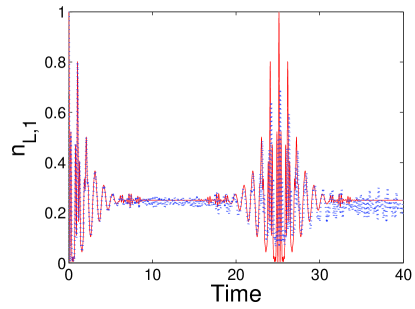
Figure 4: (Color online) $n_{L,1}$ as a function of time. The red solid curve is for result Eq. (13). The blue dotted curve is for exact numerical simulations with the full Hamiltonian of Eq. (1). $\Omega=2.4,J=0.6,g_{11}=g_{22}=0,g_{12}=g=0.2$, and $N=6$. Time is in units of $1/g$.

The general case can be attacked numerically. In Fig. 5, we show our numerical results for $n_{L,1}$ as function of time. The parameters are chosen so as to fall into the intermediate regime. For comparison, we also show the results of the strong coupling-tunneling case. We can see that, with appropriate nonlinearity, the dynamics of $n_{L,1}$ exhibit completely different and more complicated patterns than the strong coupling-tunneling case. The nonlinearity not only reduces the oscillation amplitude but also destroys the periodicity note1 . This reduction in the amplitude is due to the effective damping which is a common feature in interacting condensates sun1 ; sun2 .

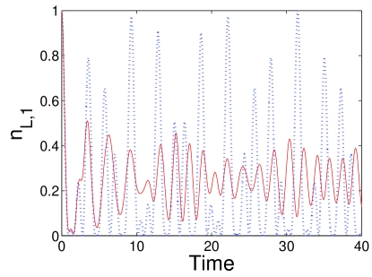
Figure 5: $n_{L,1}$ as a function of time using exact numerical simulations with the full Hamiltonian of Eq. (1). $\Omega=1,J=1.7$, $N=6$. The red solid curve is for $g11=g22=0.45$ and $g12=0.3$. The blue dotted curve is for the noninteracting case $g11=g22=g12=0$.

Now we briefly discuss a possible experimental implementation of our proposal. Our model can be conveniently realized in an optical super-lattice by superimposing two-color lasers phil ; bloch1 . Each lattice site consists of a double well potential. $J$ is determined from the shape of the double well which can be tuned by engineering the ratio of the two laser intensities. The $s$-wave scattering $g_{ij}$ can be tuned by using the well established Feshbach resonance. $\Omega$ can be tuned by changing the intensities of two microwave/RF fields both of which are coupled to the third intermediate level with a large detuning, which can be adiabatically eliminated. The relative strength in our model Hamiltonian can thus be tuned over a wide range. For the CR as shown in Fig. 4, we give an order of magnitude estimate of typical experimental parameters here. If we approximate each lattice site as a harmonic trap with trapping frequency $\omega\sim 10$kHz. The intra-species interaction strength $g$ can be tuned to be $\sim 100$Hz with the corresponding $a_{12}\simeq 25a_{B}$ ($a_{B}$ is the Bohr radius). The Josephson tunnelling rate $J$ and the coupling strength $\Omega$ is $300$Hz and $1.2$kHz, respectively, both of which can be implemented using the state-of-the-art technology.

IV conclusion

To conclude, we have studied the dynamics of a two-species Bose-Einstein condensate in a double well. Such a system is characterized by the following three factors. (1) The $s$-wave scattering $-$ $a_{11}$ and $a_{22}$ for intra-species scattering and $a_{12}$ for inter-species scattering; (2) Josephson tunnelling between the two wells; (3) population transfer between the two species driven by a resonant microwave field. We discuss the dynamics for three interesting regimes where we can obtain analytical results. (a) The strong coupling /tunnelling regime where the nonlinearity is negligible. We find the net effect of the coupling/tunnelling is either constructive or destructive; (b) the strong nonlinearity regime where Josephson tunnelling is suppressed and the system behaves like a simple two-level system; (c) the intermediate regime. For this case we only consider a specific example of vanishing intra-species scattering and weak inter-species scattering. We find collapses and revivals in the population dynamics. For the general case, we attack this problem numerically. We find the dynamics is rather complicated. The nonlinearity forces the system out of periodicity. We hope our work can be helpful to the study of quantum coherence of two-species BECs.

We deeply appreciate Dr. F. Robicheaux at Auburn University and Dr. L. You at Georgia Institute of Technology for enlightening discussions and helpful comments on the manuscript. We also thank J. Ludlow for proof reading our manuscript. This work is supported by grants with NSF.

V appendix

In this appendix, we show the procedure to derive $\langle f_{1}^{\dagger}f_{2}\rangle$. Other average values can be derived along similar lines.

$$\langle f_{1}^{\dagger}f_{2}\rangle = {1\over 4^{N}}\sum_{mnpq}\delta_{N,m+n+p+q}{N!\over m!(n-1)!p!q!}$$

$$e^{i(E_{m+1,p}+E_{n-1,q}-E_{m,p}-E_{n,q})t}$$

$$= {N\over 4^{N}}\sum_{mnpq}\delta_{N-1,m+n-1+p+q}{(N-1)!\over m!(n-1)!p!q!}$$

$$e^{i(E_{m+1,p}+E_{n-1,q}-E_{m,p}-E_{n,q})t}$$

$$= {N\over 4^{N}}\sum_{mnpq}\delta_{N-1,m+n-1+p+q}{(N-1)!\over m!(n-1)!p!q!}$$

$$e^{it(2(\Omega+J)+g/4)}e^{it{g\over 4}(m-n+2p-2q)}$$

$$= e^{it2(\Omega+J)}{N\over 4^{N}}\sum_{mnpq}{1\over 2\pi}\int_{0}^{2\pi}e^{i(m+n-1+p+q-(N-1))\phi}d\phi$$

$${(N-1)!\over m!(n-1)!p!q!}e^{it{g\over 4}(m-(n-1)+2p-2q)}$$

$$= e^{it2(\Omega+J)}{N\over 4^{N}}(N-1)!{1\over 2\pi}\int_{0}^{2\pi}d\phi e^{-i(N-1)\phi}$$

$$\sum_{mnpq}e^{im\phi}{e^{itmg/4}\over m!}e^{i(n-1)\phi}{e^{-it(n-1)g/4}\over(n-1)!}$$

$$e^{ip\phi}{e^{itpg/2}\over p!}e^{iq\phi}{e^{-itqg/2}\over q!}$$

$$= e^{it2(\Omega+J)}{N\over 4^{N}}(N-1)!{1\over 2\pi}\int_{0}^{2\pi}d\phi e^{-i(N-1)\phi}$$

$${\rm exp}[e^{i\phi+i(tg/4)}]{\rm exp}[e^{i\phi-i(tg/4)}]$$

$${\rm exp}[e^{i\phi+i(tg/2)}]{\rm exp}[e^{i\phi-i(tg/2)}]$$

$$= e^{it2(\Omega+J)}{N\over 4^{N}}(N-1)!{1\over 2\pi}\int_{0}^{2\pi}d\phi e^{-i(N-1)\phi}$$

$$\exp[e^{i\phi}2(\cos(tg/4)+\cos(tg/2))]$$

$$= e^{it2(\Omega+J)}{N\over 4^{N}}(N-1)!{1\over 2\pi}\int_{0}^{2\pi}d\phi e^{-i(N-1)\phi}$$

$$\sum_{k}{1\over k!}e^{ik\phi}2^{k}(\cos(tg/4)+\cos(tg/2))^{k}$$

$$= e^{it2(\Omega+J)}{N\over 4^{N}}(N-1)!$$

$${1\over(N-1)!}2^{N-1}(\cos(tg/4)+\cos(tg/2))^{N-1}$$

$$= e^{it2(\Omega+J)}{N\over 4}\left({\cos(tg/4)+\cos(tg/2)\over 2}\right)^{N-1}$$

References

- (1) C. J. Myatt, E. A. Burt, R. W. Ghrist, E. A. Cornell, and C. E. Wieman, Phys. Rev. Lett. 78, 586 (1997).
- (2) D. S. Hall, M. R. Matthews, J. R. Ensher, C. E. Wieman, and E. A. Cornell, Phys. Rev. Lett. 81, 1539 (1998).
- (3) D. S. Hall, M. R. Matthews, C. E. Wieman, and E. A. Cornell, Phys. Rev. Lett. 81, 1543 (1998).
- (4) H.-J. Miesner, D. M. Stamper-Kurn, J. Stenger, S. Inouye, A. P. Chikkatur, and W. Ketterle, Phys. Rev. Lett. 82, 2228 (1999).
- (5) D. M. Stamper-Kurn, H.-J. Miesner, A. P. Chikkatur, S. Inouye, J. Stenger, and W. Ketterle, Phys. Rev. Lett. 83, 661 (1999).
- (6) M. R. Matthews, B. P. Anderson, P. C. Haljan, D. S. Hall, M. J. Holland, J. E. Williams, C. E. Wieman, and E. A. Cornell, Phys. Rev. Lett. 83, 3358 (1999).
- (7) J. Williams, R. Walser, J. Cooper, E. Cornell, and M. Holland, Phys. Rev. A 59, R31 (1999).
- (8) P. Maddaloni, M. Modugno, C. Fort, F. Minardi, and M. Inguscio, Phys. Rev. Lett. 85, 2413 (2000).
- (9) G. Modugno, G. Ferrari, G. Roati, R. J. Brecha, A. Simoni, and M. Inguscio, Science 294, 1320 (2001).
- (10) M. Mudrich, S. Kraft, K. Singer, R. Grimm, A. Mosk, and M. Weidemüller, Phys. Rev. Lett. 88, 253001 (2002).
- (11) G. Modugno, M. Modugno, F. Riboli, G. Roati, and M. Inguscio, Phys. Rev. Lett. 89, 190404 (2002).
- (12) S. B. Papp, J. M. Pino, and C. E. Wieman, Phys. Rev. Lett. 101, 040402 (2008).
- (13) Tin-Lun Ho and V. B. Shenoy, Phys. Rev. Lett. 77, 3276 (1996).
- (14) C. K. Law, H. Pu, N. P. Bigelow, and J. H. Eberly, Phys. Rev. Lett. 79, 3105 (1997).
- (15) H. Pu and N. P. Bigelow, Phys. Rev. Lett. 80, 1130 (1998).
- (16) H. Pu and N. P. Bigelow, Phys. Rev. Lett. 80, 1134 (1998).
- (17) K. V. Krutitsky and R. Graham, Phys. Rev. Lett. 91, 240406 (2003).
- (18) K. M. Mertes, J. W. Merrill, R. Carretero-González, D. J. Frantzeskakis, P. G. Kevrekidis, and D. S. Hall, Phys. Rev. Lett. 99, 190402 (2007).
- (19) R. Mark Bradley, James E. Bernard, and L. D. Carr, Phys. Rev. A 77, 033622 (2008).
- (20) S. Ronen, J. L. Bohn, L. E. Halmo, and M. Edwards, Phys. Rev. A 78, 053613 (2008).
- (21) R. Navarro, R. Carretero-González, and P.G. Kevrekidis, to appear in Phys. Rev. A 2009.
- (22) Ping Zhang, C K Chan, Xiang-Gui Li, and Xian-Geng Zhao, J. Phys. B: At. Mol. Opt. Phys. 35, 4647 (2002).
- (23) X. X. Liu, H. Pu, B. Xiong, W. M. Liu, and J. B. Gong, Phys. Rev. A 79, 013423 (2009).
- (24) X. F. Zhang, X. H. Hu, X. X. Liu, and W. M. Liu, Phys. Rev. A 79, 033630 (2009);
- (25) D. Gordon and C. M. Savage, Phys. Rev. A 59, 4623 (1999).
- (26) J. Williams, R. Walser, J. Cooper, E. Cornell, and M. Holland, Phys. Rev. A 59, R31 (1999).
- (27) Le-Man Kuang and Zhong-Wen Ouyang, Phys. Rev. A 61, 023604 (2000).
- (28) Wei-Dong Li, X. J. Zhou, Y. Q. Wang, J. Q. Liang, and Wu-Ming Liu, Phys. Rev. A 64, 015602 (2001).
- (29) L. You, Phys. Rev. Lett. 90, 030402 (2003).
- (30) Z.-D. Chen, J.-Q. Liang, S.-Q. Shen, and W.-F. Xie, Phys. Rev. A 69, 023611 (2004).
- (31) H. T. Ng, C. K. Law, and P. T. Leung, Phys. Rev. A 68, 013604 (2003).
- (32) Guo-feng Zhang, Shu-shen Li, and Jiu-qing Liang, Phys. Scr. 72, 274 (2005).
- (33) Weibin Li,, Wenxing Yang, Xiaotao Xie, Jiahua Li, and Xiaoxue Yang, J. Phys. B: At. Mol. Opt. Phys. 39, 3097 (2006).
- (34) N. Teichmann and C. Weiss, EPL 78, 10009 (2007).
- (35) Indubala I. Satija, Radha Balakrishnan, Phillip Naudus, Jeffrey Heward, Mark Edwards, and Charles W. Clark, Phys. Rev. A 79, 033616 (2009).
- (36) A. Smerzi, S. Fantoni, S. Giovanazzi, and S. R. Shenoy, Phys. Rev. Lett. 79, 4950 (1997).
- (37) S. Raghavan, A. Smerzi, S. Fantoni, and S. R. Shenoy, Phys. Rev. A 59, 620 (1999).
- (38) Augusto Smerzi and Srikanth Raghavan, Phys. Rev. A 61, 063601 (2000).
- (39) R. Qi, X. L. Yu, Z. B. Li, and W. M. Liu, Phys. Rev. Lett. 102, 185301 (2009).
- (40) E. M. Wright, D. F. Walls, and J. C. Garrison, Phys. Rev. Lett. 77, 2158 (1996).
- (41) In the strong coupling/tunnelling regime, the exact periodicity only exists for commensurable and . Assuming and are the smallest integers satisfying , the period is where denotes the minimum of and .
- (42) B. Sun, M. S. Pindzola, and L. You, Phys. Rev. A 79, 033608 (2009).
- (43) B. Sun and M. S. Pindzola, J. Phys. B: At. Mol. Opt. Phys. 42, 145502 (2009).
- (44) S. Peil, J. V. Porto, B. Laburthe Tolra, J. M. Obrecht, B. E. King, M. Subbotin, S. L. Rolston, and W. D. Phillips, Phys. Rev. A 67, 051603(R) (2003).
- (45) S. Fölling, S. Trotzky, P. Cheinet, M. Feld, R. Saers, A. Widera, T. Müller, and I. Bloch, Nature (London) 448, 1029 (2007).