The mass ratio and formation mechanisms of Herbig Ae/Be star binary systems

Abstract

We present B and R band spectroastrometry of a sample of 45 Herbig Ae/Be stars in order to study their binary properties. All but one of the targets known to be binary systems with a separation of $\rm\sim 0.1-2.0$ arcsec are detected by a distinctive spectroastrometric signature. Some objects in the sample exhibit spectroastrometric features that do not appear attributable to a binary system. We find that these may be due to light reflected from dusty halos or material entrained in winds. We present 8 new binary detections and 4 detections of an unknown component in previously discovered binary systems. The data confirm previous reports that Herbig Ae/Be stars have a high binary fraction, $\rm{74\pm 6}$ per cent in the sample presented here. We use a spectroastrometric deconvolution technique to separate the spatially unresolved binary spectra into the individual constituent spectra. The separated spectra allow us to ascertain the spectral type of the individual binary components, which in turn allows the mass ratio of these systems to be determined. In addition, we appraise the method used and the effects of contaminant sources of flux. We find that the distribution of system mass ratios is inconsistent with random pairing from the Initial Mass Function, and that this appears robust despite a detection bias. Instead, the mass ratio distribution is broadly consistent with the scenario of binary formation via disk fragmentation.

1 Introduction

Our understanding of the formation and early evolution of massive stars ($\rm M_{*}\ga 8M_{\odot}$) is much less complete than in the case of low mass stars. The scenario of low mass star formation has been relatively well studied, and a broadly consistent observational and theoretical picture has now emerged. The various phases of low mass star formation include: cloud collapse, proto-stellar creation and a subsequent contraction of Pre Main Sequence (PMS) objects towards the Zero Age Main Sequence (ZAMS). This later stage, the T Tauri phase, is easy to observe and therefore relatively well understood (Bouvier et al., 2007). In the case of more massive stars the situation is much less clear. Such stars do not experience an optically visible PMS phase, evolve on a much more rapid timescale, and are considerably more luminous than low mass stars. Early studies on the effects of radiation pressure and the considerable ionising output of massive young stars prompted speculation that massive star formation might proceed in a different manner to that of low mass stars (Larson & Starrfield, 1971; Kahn, 1974). For example, it has been suggested that the most massive stars form via stellar mergers or competitive accretion (Bally & Zinnecker, 2005).

However, recent work, on both the observational and theoretical front, suggests that massive star formation may not be dissimilar to low mass star formation. As an example of observational results, Patel et al. (2005) report the detection of a massive disk around a 15$\rm M_{\odot}$ protostar, indicating that massive stars may form via monolithic accretion. On the theoretical front, recent work indicates accretion onto a massive protostar is not impeded by radiation pressure (Yorke & Sonnhalter, 2002; Turner et al., 2007; Krumholz et al., 2009). However, while significant progress has been made, there remain many unaddressed questions related to the formation and evolution of massive stars (Zinnecker & Yorke, 2007). As observations of massive young stars are challenging, the full extent of the differences and similarities between low and high mass star formation are still unknown.

Between the two extremes of mass lie the Herbig Ae/Be (HAe/Be) stars (Herbig, 1960). These stars represent the most massive of objects to experience an optically visible PMS evolutionary phase. Therefore, HAe/Be stars offer an opportunity to study the early evolution of stars more massive than the sun. Spectropolarimetry indicates that Herbig Ae stars may undergo a PMS phase similar to that of the T Tauri stars, while Herbig Be stars may evolve via disk accretion, rather than magnetospheric accretion (Vink et al., 2002, 2005a; Mottram et al., 2007). Therefore, it appears that a transition in formation mechanisms occurs across the HAe/Be mass boundary (Mottram et al., 2007). However, the critical mass has not yet been established.

To examine the similarities and differences between low mass T Tauri stars, HAe/Be stars and the optically invisible Massive Young Stellar Objects (MYSOs), study of the circumstellar environment at small angular scales is required. This is not trivial, requiring observations with high angular resolution (Mannings & Sargent, 1997; Fuente et al., 2006; Grady, 2007; Kraus et al., 2008). Despite the progress in the field, a full understanding of HAe/Be stars is hampered by the small sample sizes involved. By way of contrast, Baines et al. (2006) utilised spectroastrometry to study a large sample of HAe/Be stars with milli-arcsecond (mas) precision. Despite this resolution Baines et al. (2006) did not detect any accretion disks around HAe/Be stars. However, they did find that the majority, $\rm{68\pm 11}$ per cent, of HAe/Be stars reside in relatively wide (probably a few-hundred au, see Section 5.3) binary systems.

The binary fraction reported by Baines et al. (2006) is greater than that of T Tauri stars at similarly wide separations, which in turn is greater than that of Main Sequence G-dwarfs at the same separations (Duquennoy & Mayor, 1991; Reipurth & Zinnecker, 1993; Ghez et al., 1993). Indeed, this high binary fraction is approaching that of more massive stars (Preibisch et al., 1999). However, little is known about the properties of such binary systems. The properties of the binary components and configurations of such systems are of interest as they can constrain the binary formation mechanism. The seminal study to date is that by Bouvier & Corporon (2001), who used Adaptive Optics assisted observations to construct Spectral Energy Distributions (SEDs) for each component in a number of HAe/Be binary systems. The drawback of SED fitting is that PMS stars, as young stars, are inevitably associated with dusty, obscured environments. Therefore, the brightness ratio of a binary determined by SED fitting can occasionally be ambiguous. However, very few HAe/Be binary systems have been studied with spatially resolved spectroscopy, and thus far such studies have been conducted with seeing limited resolution (Carmona et al., 2007; Hubrig et al., 2007).

The position angles of HAe/Be binary systems seem to be preferentially aligned with the spectropolarimetrically detected circumprimary disks (Baines et al., 2006). This already places constraints on the formation modes of these stars, in that it seems the systems formed via fragmentation of a molecular core or disk. This had already been suggested for lower mass binaries (Wolf et al., 2001; Kroupa & Burkert, 2001), but little is known about the formation mechanisms of more massive stars. This paper describes a spectroastrometric follow-up of the work of Baines et al. (2006) with dedicated observations to study both components of binary systems. The objective is to determine the properties of these binary systems and thus place stronger, more quantitative, constraints on the formation of stars of intermediate mass. We do this by determining the mass ratio of these binary systems. This is done using a spectroastrometric technique to disentangle the constituent spectra of unresolved binary systems, allowing the spectral type, and hence mass, of each component to be determined. Spectroastrometry itself is a relatively simple technique that extracts the spatial information present in conventional longslit spectra. Crucially, spectroastrometry can probe changes in flux distributions with a typical precision of a mas or less (Bailey, 1998a), which is required to study unresolved binary systems. Typically the minimum separation probed is of the order 100 mas, as the signature of a binary system is dependant upon the system brightness ratio and separation.

This paper is structured as follows: in Section 2 we present our sample selection, observation method and data reduction procedures. In Section 3 we discuss the spectroastrometric signatures observed. In Section 4 we present the method of splitting unresolved binary spectra and in Section 4.1 we review the results of separating binary spectra into their constituent spectra. In Section 5 we discuss our results. Finally, we conclude this paper in Section 6 by summarising the salient points raised.

2 Observations and data reduction

2.1 Observations

The data presented consist of long-slit spectra in the B band ($\rm 4200-5000\rm{\AA}$) and/or the R band ($\rm 6200-7000\rm{\AA}$) of 45 HAe/Be stars, and 2 emission line objects which are possible HAe/Be stars. The objects were chosen from the catalogs of Thé et al. (1994), Vieira et al. (2003) & Hernández et al. (2004), and were selected to be reasonably bright (V $\rm\leq$ 12-13). Some objects previously observed by Baines et al. (2006) were observed to provide a consistency check on the spectroastrometric signatures. Given the small population of HAe/Be stars, the objects observed constitute a representative sample of HAe/Be stars, albeit brightness limited.

The data were obtained using the 4.2m William Herschel Telescope (WHT) and the 2.5m Isaac Newton Telescope (INT). At the WHT, data were obtained on the 6th & 7th of October 2006, using the Intermediate Dispersion Spectrograph and Imaging System (ISIS) spectrograph. Spectra of 20 objects were taken simultaneously in the B and R bands using the dichroic slide of ISIS. In most cases a slit $\rm{5}$ arcsec wide was used to ensure all the light from a given binary system entered the slit, even in poor seeing. This allows us to study the individual binary components, unlike Baines et al. (2006), who used a slit of 1 arcsec. The R1200B and R1200R gratings were used and the resulting spectral resolving power was found to be $\rm\sim 3500$, corresponding to $\rm 85\,km\,s^{-1}$. The angular pixel size was $\rm{0.20}$ and $\rm{0.22}$ arcsec in the B band and R band respectively, which means that the spatial profile of the longslit spectra was well sampled (average FWHM 1.9 arcsec). At the INT data were obtained using the 235mm camera and the Intermediate Dispersion Spectrograph (IDS). Observing was conducted from the 27th of December 2008 to the 3rd of January 2009. The spectra of 32 objects were obtained, despite adverse weather conditions preventing observing for the better part of three nights. As at the WHT the slit width was generally $\rm 5$ arcsec. The R1200R and R1200B gratings were used and the resulting spectral resolution was found to be $\rm\sim 3800$, or $\rm 80\,km\,s^{-1}$. The angular size of the pixels was $\rm{0.4}$ arcsec, which fully sampled the average spatial profile of the spectra (1.8 arcsec).

Multiple spectra were taken at four position angles (PA) on the sky. The PAs selected always comprised of two perpendicular sets of two anti-parallel angles, e.g. $\rm 0\degr$, $90^{\circ}$, $180^{\circ}$ and $270^{\circ}$. Dispersion calibration arcs were made using CuNe and CuAr lamps. Table 1 presents a summary of the observations.

Table 1: Log of the observations, column 1 lists the objects observed, column 2 denotes the spectral type of the objects, column 3 lists the V band magnitudes of the sample, and column 4 designates which telescope the object in question was observed with. Columns 5 and 6 list the average seeing conditions, columns 7 and 8 list the total exposure times and column 9 denotes the slit width used. Column 10 lists the total Signal to Noise Ratios, and finally, column 11 presents the date(s) each object was observed. Information on the objects is taken from SIMBAD (simbad.u-strasbg.fr) unless otherwise stated.

Object	Spec type	V	Telescope	$\rm\overline{FWHM}^{a}$	$\rm\overline{FWHM}^{b}$	$\rm{t_{blue}}$	$\rm{t_{red}}$	Slit	SNR	Date
				(″)	(″)	(s)	(s)	(″)
VX Cas	$\rm{A0e}$	11.3	WHT	1.3	1.2	4800	4800	5.0	$\rm{600_{B}}$,$\rm{570_{R}}$	07/10/2006
VX Cas	$\rm{A0e}$	11.3	INT	1.1	1.7	2800	3600	$\rm 2.5_{\rm B},5.0_{\rm R}$	$\rm{370_{B}}$,$\rm{370_{R}}$	28/12/2008,31/12/2008
V594 Cas	Be	10.6	INT	1.3	–	3200	–	5.0	610	01/01/2009
V1185 Tau	A1	10.7	INT	1.7	–	3200	–	5.0	430	03/01/2009
IP Per	$\rm{A3}$	10.3	INT	1.2	1.4	2000	2400	$\rm 2.5_{\rm B},5.0_{\rm R}$	$\rm{110_{B}}$,$\rm{320_{R}}$	28/12/2008,31/12/2008
AB Aur	A0Vpe	7.1	WHT	1.9	1.9	330	320	5.0	$\rm{110_{B}}$,$\rm{650_{R}}$	06/10/2006
MWC 480	$\rm{A3pshe}$	7.7	WHT	2.0	2.1	960	640	5.0	$\rm{1100_{B}}$,$\rm{800_{R}}$	06/10/2006
UX Ori	$\rm{A3e}$	9.6	WHT	2.4	2.4	3600	3600	5.0	$\rm{1200_{B}}$,$\rm{940_{R}}$	06/10/2006
V1012 Ori	$\rm{Be^{c}}$	12.1	INT	2.1	–	4800	–	5.0	150	02/01/2009
V1366 Ori	A0e	9.8	INT	1.3	–	2400	–	3.0	570	31/12/2008
V346 Ori	$\rm{A5III}$	10.1	INT	1.5	–	3600	–	5.0	200	01/01/2009
HD 35929	A5	8.1	WHT	1.9	1.7	2060	1470	5.0	$\rm{40_{B}}$,$\rm{900_{R}}$	07/10/2006
V380 Ori	A0	10.7	INT	1.5	1.6	3600	2940	$\rm 3.0_{\rm B},5.0_{\rm R}$	$\rm{100_{B}}$,$\rm{200_{R}}$	28/12/2008,31/12/2008
MWC 758	A3e	8.3	WHT	1.4	1.3	1080	960	5.0	$\rm{50_{B}}$,$\rm{660_{R}}$	07/10/2006
HK Ori	A4pev	11.9	INT	2.4	–	4800	–	5.0	200	02/01/2009
HD 244604	A3	9.4	WHT	1.7	1.6	3180	3660	5.0	$\rm{100_{B}}$,$\rm{720_{R}}$	07/10/2006
V1271 Ori	A5	10.0	INT	1.6	–	2460	–	5.0	410	01/01/2009
T Ori	A3	9.5	INT	1.9	–	3200	–	5.0	300	03/01/2009
V586 Ori	$\rm{A2V}$	9.8	INT	3.3	–	2940	–	5.0	650	02/01/2009
HD 37357	A0e	8.8	INT	1.4	1.4	2060	1470	$\rm 3.0_{\rm B},5.0_{\rm R}$	$\rm{200_{B}}$,$\rm{350_{R}}$	28/12/2008,31/12/2008
V1788 Ori	B9Ve	9.9	INT	1.7	–	1350	–	5.0	450	01/01/2009
HD 245906	B9IV	10.7	INT	1.8	–	2800	–	5.0	100	03/01/2009
RR Tau	A2II-IIIe	10.9	INT	1.7	–	2800	–	5.0	250	03/01/2009
V350 Ori	A0e	10.4(B)	INT	1.9	–	4800	–	5.0	130	03/01/2009
MWC 120	A0	7.9	WHT	2.1	1.9	480	480	5.0	$\rm{1500_{B}}$,$\rm{690_{R}}$	06/10/2006
MWC 120	A0	7.9	INT	1.4	1.6	2460	1250	$\rm 3.0_{\rm B},5.0_{\rm R}$	$\rm{1200_{B}}$,$\rm{560_{R}}$	28/12/2008,31/12/2008
MWC 790	Be	12.0	INT	3.1	–	4050	–	5.0	200	02/01/2009
MWC 137	Be	11.2	INT	–	2.1	–	4560	5.0	200	28/12/2008
HD 45677	$\rm{Bpshe}$	8.0	WHT	2.0	1.9	360	240	5.0	$\rm{900_{B}}$,$\rm{550_{R}}$	06/10/2006
LkH$\rm\alpha$ 215	B7.5e	10.6	INT	1.5	2.3	3600	3600	$\rm 5.0_{\rm B},4.0_{\rm R}$	$\rm{300_{B}}$,$\rm{360_{R}}$	27/12/2008,31/12/2008
MWC 147	$\rm{B6pe}$	8.8	WHT	1.8	1.5	3000	1700	5.0	$\rm{1200_{B}}$,$\rm{500_{R}}$	07/10/2006
MWC 147	$\rm{B6pe}$	8.8	INT	1.3	–	2400	–	5.0	620	01/01/2009
R Mon	B0	10.4	INT	4.2	2.5	3600	3600	5.0	$\rm{100_{B}}$,$\rm{240_{R}}$	28/12/2008,02/01/2009
V590 Mon	B8pe	12.9	INT	1.5	–	2670	–	5.0	200	01/01/2009
V742 Mon	B2Ve	6.9	INT	1.4	2.8	1740	2535	5.0	$\rm{400_{B}}$,$\rm{800_{R}}$	30/12/2008,31/12/2008
OY Gem	Bp[e]	11.1	INT	1.8	–	2880	–	5. 0	100	03/01/2009
GU CMa	$\rm{B2Vne}$	6.6	WHT	2.5	2.4	360	360	5.0	$\rm{1500_{B}}$,$\rm{900_{R}}$	06/10/2006
GU CMa	$\rm{B2Vne}$	6.6	INT	1.8	–	720	–	5.0	1400	03/01/2009
MWC 166	B0IVe	7.0	WHT	2.5	2.3	210	120	5.0	$\rm{1200_{B}}$,$\rm{800_{R}}$	06/10/2006
HD 76868	B5	8.0	INT	1.5	2.4	4830	2100	5.0	$\rm{100_{B}}$,$\rm{100_{R}}$	30/12/2008,01/01/2009
HD 81357	B8	8.4	INT	1.7	–	4800	–	5.0	100	03/01/2009
MWC 297	$\rm{Be}$	12.3	WHT	1.4	1.2	4100	3120	5.0	$\rm{100_{B}}$,$\rm{500_{R}}$	07/10/2006
HD 179218	B9e	7.2	WHT	2.6	2.4	2100	1200	1.0/1.5	$\rm{2300_{B}}$,$\rm{940_{R}}$	06/10/2006
HD 190073	$\rm{A2IVpe}$	7.8	WHT	1.5	1.2	540	360	5.0	$\rm{600_{B}}$,$\rm{800_{R}}$	07/10/2006
BD +40 4124	B2	10.7	WHT	2.1	1.9	600	660	4.0	$\rm{500_{B}}$,$\rm{370_{R}}$	07/10/2006
MWC 361	$\rm{B2Ve}$	7.4	WHT	1.7	1.7	1350	960	2.5/4.0	$\rm{1400_{B}}$,$\rm{1400_{R}}$	06/10/2006
SV Cep	$\rm{Ae}$	10.1(B)	INT	1.6	–	3000	–	5.0	600	02/01/2009
MWC 655	B1IVnep	9.2	INT	1.7	–	2400	–	5.0	400	03/01/2009
Il Cep	$\rm{B2IV/Ve}$	9.3	WHT	1.4	1.2	3500	3000	5.0	$\rm{800_{B}}$,$\rm{500_{R}}$	07/10/2006
BHJ 71	B4e	10.9	WHT	1.8	1.8	1200	1080	4.0	$\rm{500_{B}}$,$\rm{340_{R}}$	06/10/2006
BHJ 71	B4e	10.9	INT	1.7	–	4200	–	5.0	500	01/01/2009
MWC 1080	$\rm{B0}$	11.6	WHT	2.0	2.0	3300	4170	5.0	$\rm{200_{B}}$,$\rm{500_{R}}$	06/10/2006

2.2 Data reduction

Data reduction was conducted using the Image Reduction and Analysis Facility (IRAF) and routines written in Interactive Data Language (IDL). Initial data reduction consisted of bias subtraction and flat field division. The total intensity spectra were then extracted from the corrected data in a standard fashion. Wavelength calibration was conducted using the arc spectra, and the wavelength calibration solution had a precision of the order $\rm{<0.1\AA}$.

Spectroastrometry was performed by fitting Gaussian functions to the spatial profile of the long-slit spectra at each dispersion pixel. This resulted in a positional spectrum, the centroid of the Gaussian as a function of wavelength, and a Full Width at Half Maximum (FWHM) spectrum, the FWHM as a function of wavelength. Spot checks were used to ensure that a Gaussian was an accurate representation of the data. The continuum position exhibited a general trend across the CCD chip: of the order of 10 pixels in the case of the ISIS data and 2 pixels in the IDS data. This was removed by fitting a low order polynomial ($\rm{4^{th}}$ or $\rm{5^{th}}$ order) to the continuum regions of the spectrum.

All intensity, positional and FWHM spectra at a given PA were combined to make an average spectrum for each PA. A correction for slight changes in the dispersion across PAs was determined by cross-correlating average intensity spectra obtained at different PAs. The correction was then applied to the average intensity, positional and FWHM spectra. The average positional spectra for anti-parallel PAs were then combined to form the average, perpendicular, position spectra, for example: ($\rm 0^{\circ}-180^{\circ}$)/2 and ($\rm 90^{\circ}-270^{\circ}$)/2. This procedure eliminates instrumental artifacts as real signatures rotate by $\rm 180^{\circ}$ when viewed at the anti-parallel PA, while artifacts remain at a constant orientation. In addition, all positional spectra were visually inspected for artifacts not fully removed by this procedure. As with the positional spectra, the FWHM spectra at anti-parallel PAs were also combined to make two averaged, perpendicular spectra. While FWHM features do not rotate across different PAs, the features observed at anti-parallel PAs were used to exclude artifacts via a visual comparison. All conditions being constant, a real FWHM signature should not change from one PA to the opposite angle at $\rm+180^{\circ}$.

3 Spectroastrometric signatures

3.1 Binary spectroastrometric signatures over H i lines

An unresolved binary system, in which each component has a unique spectrum, displays a clear signature in the behaviour of the spectral photocentre. As the spatial profile is the sum of the two stars convolved with the seeing, the peak is not located at the position of either star, but somewhere between the components. The exact location of the photo-centre depends on the intensity ratio and the separation of the two components. Over spectral lines the binary flux ratio changes from its continuum value, which results in the peak position shifting towards the dominant component. Therefore, unresolved binary systems are revealed by a displacement in the positional spectrum over spectral line. In addition, an unresolved binary system is also revealed by a change in the FWHM over lines in the spectrum. Again, this is because the spatial profile of an unresolved binary system is dependent upon the binary flux ratio, which changes from its continuum value across certain lines. As the error in the centre of the Gaussian profile is governed by photon statistics, changes of mas scales can be traced. This allows binary systems with separations as small as $\rm{\sim 0.1}$ arcsec and differences in brightness up to 5 magnitudes to be studied (Baines et al., 2006).

To illustrate the detection of a binary system the observations of GU CMa are presented in some detail. GU CMa is known to be a Herbig Be binary system with a separation of $\rm\sim 0.65$ arcsec, a PA of $\rm\sim 195^{\circ}$, a brightness difference between components of 0.7-1.0 magnitudes in the optical band and a primary with a spectral type of B1 (Fu et al., 1997; Fabricius & Makarov, 2000; Bouvier & Corporon, 2001).

GU CMa presents a very clear binary signature in the spectroastrometric observations (Fig. 1). Across the H i lines the photo-centre of the spectrum clearly shifts towards the North-East. This demonstrates that the primary, the component brightest in the continuum, dominates the emission spectrum. It also indicates that the secondary, the component least bright in the continuum, has the larger absorption profile of H$\rm\gamma$. As the photo-centre shifts to the North-East the FWHM of the spectrum is seen to decrease. This also indicates that the primary dominates the spectrum at these particular wavelengths. The photo-centre is also observed to shift to the North-East across the He  i lines. This again indicates that it is the primary that dominates the binary flux over this line.

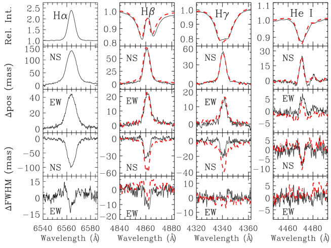
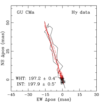
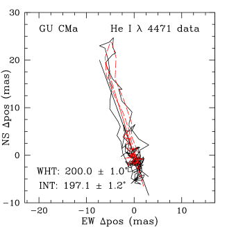
Figure 1: The spectroastrometric signature of GU CMa. In the top panel, presented from left to right: the H$\rm\alpha$, H$\rm\beta$, H$\rm\gamma$ and He i $\rm\lambda 4471$ spectral profiles and associated spectroastrometric signatures. In the spectroastrometric signatures North and East are positive. In the lower section of the figure we present the associated XY-plots of the H$\rm\alpha$, H$\rm\beta$, H$\gamma$, and by way of contrast, the He i $\rm\lambda$ 4471 spectroastrometric displacements. In the XY-plots North is up and East is to the left. The data from the WHT is represented by the solid lines, while the data obtained at the INT is represented by the dashed lines. Note the consistency between the two datasets.

All the spectroastrometric excursions across the H i lines produce a PA consistent to within $\rm\sim 1^{\circ}$. The agreement between the spectroastrometric displacements across different lines is an important consistency check. In addition, the close agreement between the data gathered at different telescopes provides compelling evidence that the signatures observed are real and not contaminated by instrumental affects. The difference in the FWHM changes can be explained by the difference in the seeing between observations. Finally, that our observations concur with the results of Baines et al. (2006), further proves that these signatures are real and no instrumental effect. As demonstrated by the spectroastrometric signature associated with the He i line such features do not solely occur across lines with an emission component. This is important to note as it means the spectra splitting method does not require emission lines to separate spectra.

In the case of some stars significant FWHM changes are observed which are not accompanied by a change in the spectral photo-centre. Baines et al. (2006) regard such a signature as a possible binary detection. This is substantiated as Baines et al. (2006) demonstrate that the spectroastrometric signature of a binary system with a separation of greater than half the slit width exhibits larger FWHM than positional features. However, in the data presented here, this scenario is unlikely. As a wide slit was used, a binary with a separation of half the slit width would be resolved, even in seeing conditions of 2 arcsec. As a resolved system does not exhibit a spectroastrometric signature we suspect there may be an alternative explanation to the FWHM features not accompanied by positional features. We note that such features are not instrumental as some stars exhibit no change in FWHM over spectral lines. In many cases the large FWHM features occur over absorption features in the emission profiles. This suggests that these features may trace an extended structure which scatters the line profile, rather than being an intrinsic source. If the scattering media were close to being symmetrically distributed around the central star it could generate a large FWHM increase while not resulting in a positional signature. Such sources of flux could be a disk/stellar wind (Azevedo et al., 2007), the halos reported by Leinert et al. (2001) and Monnier et al. (2006), or nebulosity. This topic will be returned to in Section 5.1.

The observational results naturally fall into three categories: clear binary signatures, possible binary/other signatures and null detections. We present a summary of the detections in our results in Table 2, in which we separate known binary systems and new spectroastrometric detections. It is important to note that it is not only binaries that are detected by spectroastrometry, optical outflows and disks can also result in a spectroastrometric feature (Bailey, 1998b; Takami et al., 2001). However, there are no disk signatures, and only a few detections of outflows, in the data presented here.

There are 29 stars in our sample that are referred to in the literature as being part of a binary system. However, we exclude AB Aur and HD 244604 as the binary nature of these objects is open to question, section 5.1 explains why this is the case. We detect 20 of the 27 previously known binary systems. As six of the seven undetected systems have separations greater than $\rm{2}$ arcsec and/or brightness differences as great as 8 magnitudes, we detect all but one, UX Ori, of the binary systems that we would expect to detect. Given that the majority of known binary systems are detected, objects which are not known to be part of a binary system but exhibit similar spectroastrometric signatures to the known binary systems are classified as new binary detections. We detect 8 new binary systems. The raw binary fraction of the sample is 0.60. Including the non detections of known binary systems the binary fraction of the sample is 0.74. While these figures are high for a limited separation range, they are consistent with previous work (Pirzkal et al., 1997; Baines et al., 2006).

As expected, we do not detect the binaries with separations greater than $\rm{\sim 2.0}$ arcsec and differences in brightness greater than $\rm{5}$ magnitudes, e.g. HD 179218 and MWC 297. We note that the wide companions are not detected in the longslit spectra as distinct sources. VX Cas, T Ori, LkH$\rm\alpha$ 215 and Il Cep are all known to be binary systems and all display a binary signature in their spectroastrometric signatures. Therefore, these stars are classified above as detections of known binary systems. However, these systems are wide binaries with separations greater than 5 arcsec. These companions are clearly resolvable, and thus the spectroastrometric signatures we observe can not be due to the previously reported companion. Therefore, we suggest we have detected previously unknown companions to VX Cas, T Ori, LkH$\rm{\alpha}$ 215 and Il Cep.

Table 2: Previously known binary systems and new detections. Column 1 list the objects in question, columns 2 and 3 list the separation and PA of the known binaries, taken from the literature. Column 4 contains difference in brightness between the two binary components. The amalgamation of data is not complete, if more than one value of binary parameter is available in the literature, only one is presented for the sake of clarity.

Object	Separation	PA	$\rm\Delta flux$
	(mas)	(∘)	(magnitudes)
Known binaries detected:
VX Cas	$\rm{5340^{A}}$	$\rm{{165.3}^{A}}$	K:$\rm{4.8}^{A}$
V380 Ori	$\rm{125\pm 25^{B}}$	$\rm{224.0\pm 2.0^{B}}$	K:$\rm{1.42^{B}}$
HK Ori	$\rm{347.7\pm 2.5^{B}}$	$\rm{41.8\pm 0.7^{B}}$	V: $\rm{0.87^{B}}$
T Ori	$\rm{7700\pm 200^{C}}$ and $\rm{{spectroscopic}^{D}}$	$\rm{72.6^{C}}$	K:$\rm{>4.5^{C}}$
V586 Ori	$\rm{990^{A}}$	$\rm{30.3^{A}}$	K:$\rm{2.8^{A}}$
HD 37357	$\rm{186^{E}}$	$\rm{49.0^{E}}$	K:$\rm{1.7^{A}}$
V1788 Ori	$\rm{520^{A}}$	$\rm{352.9^{A}}$	K:$\rm{3.5^{A}}$
HD 245906	$\rm{130^{A}}$	$\rm{77.1^{A}}$	K:$\rm{1.5^{A}}$
V350 Ori	$\rm{290^{A}}$	$\rm{206.8^{A}}$	K:$\rm{3.2^{A}}$
HD 45677		$\rm{150\pm 17^{F}}$
LkH$\rm\alpha$ 215	$\rm{8500^{A}}$	$\rm{226.6^{A}}$	K:$\rm{4.8^{A}}$
MWC 147	$\rm{150^{A}}$	$\rm{55.6^{A}}$	K:$\rm{3.8^{A}}$
R Mon	$\rm{670^{G}}$	$\rm{290.7^{G}}$	K:$\rm{{4.9^{A}}}$
GU CMa	$\rm{654^{H}}$	$\rm{194.5^{H}}$	V:$\rm{0.95\pm 0.02^{H}}$
MWC 166	$\rm{654^{H}}$	$\rm{297.8^{H}}$	V:$\rm{1.41^{H}}$
BD +40 4124	$\rm{720^{A}}$	$\rm{175.1^{A}}$	K:$\rm{5.4^{A}}$
MWC 361	$\rm{2250\pm 240^{I}}$	$\rm{164.0\pm 1.0^{I}}$	K:$\rm{{4.9}^{I}}$
$\rm{SV\,Cep^{J}}$
Il Cep	$\rm{6960^{I}}$	$\rm{147.0^{I}}$	K:$\rm{0.0^{I}}$
MWC 1080	$\rm{760\pm 2^{C}}$	$\rm{267.0\pm 1.0^{C}}$	K:$\rm{3.25\pm 0.08^{4}}$
Known binaries not detected:
UX Ori	$\rm{22(min)^{K}}$	$\rm{257.4\pm 18.4^{K}}$
MWC 758	$\rm{2280^{A}}$	$\rm{311.3^{A}}$	K:$\rm{8.3^{A}}$
V1271 Ori	$\rm{8380^{A}}$	$\rm{294.7^{A}}$	K$\rm{6.7^{A}}$
V590 Mon	$\rm{5007^{A}}$	$\rm{97.1^{A}}$	K$\rm{6.6^{A}}$
MWC 297	$\rm{3930\pm 200^{L}}$	$\rm{313\pm 2^{L}}$	H:$\rm{{8.5\pm 0.25}^{L}}$
HD 179218	$\rm{2540^{A}}$	$\rm{140.5^{A}}$	K:$\rm{6.6^{A}}$
BHJ 71	$\rm{6170^{A}}$	$\rm{29.2^{A}}$	K$\rm{8.3}^{A}$
New spectroastrometric detections:
V1366 Ori, HD 35929, RR Tau, MWC 120, V742 Mon, OY Gem, HD 76868 and HD 81357

Table 5 summarises the spectroastrometric signatures over H$\rm\alpha$ and H$\mathrm{\beta}$. We note that similar behaviour was observed across H$\rm\gamma$ and other lines, but to keep this paper concise we only present the H$\rm\alpha$ and H$\mathrm{\beta}$ signatures. Furthermore, the spectroastrometric signatures of the entire sample over either the H$\rm{\alpha}$ or H$\rm\beta$ lines are presented in Appendix B. Spectral variability is a common behaviour of HAe/Be stars (Rodgers et al., 2002; Mora et al., 2004). In the case of the few objects observed twice, some line profile variations are seen. However, the spectroastrometric signatures of objects observed twice are generally consistent, e.g. the example of GU CMa (Fig 1). In addition, in the case of objects common to the this sample and that of Baines et al. (2006), the spectroastrometric signatures presented here are consistent with the previous results. Therefore, we conclude that spectral variability, on timescales of years, does not effect the spectroastrometric signatures observed. No line profile variability on timescales of minutes is observed.

To summarise, spectroastrometry is a powerful tool with which to study binary systems, as GU CMa demonstrates. Not only do we clearly detect a $\rm 0.6$ arcsec binary in seeing as large as $\rm 2.5$ arcsec, we also trace the PA of the system with a precision of $\rm 1^{\circ}$ or less. Indeed, spectroastrometry detects all but one of the known binary systems with separations less than $\rm{\sim 2}$ arcsec and differences in brightness of less than 5 magnitudes. In addition, the PAs of these systems are all traced with a precision of the order of $\rm{1^{\circ}}$, and are generally consistent with literature values to within $\rm{\sim 5^{\circ}}$. Most importantly, the spectroastrometric displacements contain information as to which component of the binary system dominates the flux over certain spectral features. This information can be used to separate the constituent spectra.

3.2 Artifacts

Several spectroastrometric signatures presented in Table 5 are referred to as artifacts. An artifact is defined as a spectroastrometric signature which does not rotate by $\rm{180^{\circ}}$ when viewed at two anti-parallel position angles. Artifacts in spectroastrometric data can arise from a number of sources. Instrumental effects include: the misalignment of the dispersion axis with the CCD columns, a change in focus along the slit, curvature of the spectrum and any departure of the CCD array from a regular grid (Bailey, 1998b). As discussed in Section 2.2, such artifacts are readily identified and negated. The observation of unresolved lines can also result in false signatures (Bailey, 1998a). Here, the data were obtained with a resolution sufficient to resolve most spectral lines. However, the narrow absorption troughs in many of the double-peaked H i emission profiles may cause some of the artifacts as these features are often barely resolved.

In addition, Brannigan et al. (2006) report an artifact that is a consequence of image distortion, regardless of whether the spectral lines are well resolved. An offset between the image centre and the centre of the slit results in a change in the angle of incidence of light onto the grating, and thus a slightly blue or red shifted image. This causes a wavelength dependant change in position, and therefore an artificial spectroastrometric signature. As we use a wide slit of 5 arcsec this effect is likely to be origin of many of the artifacts present in our data.

The empirical finding is that it is crucial to obtain multiple spectra, comprising of anti-parallel sets of data. Such data will identify artifacts regardless of their cause, and can also be used to remove systematic effects.

4 Splitting binary spectra

As spectroastrometric signatures trace changes in flux distributions such signatures can be used to disentangle a convolved binary spectrum into its constituent spectra. Two approaches can be used. One method relies upon a priori information while the other does not.

The first approach was pioneered by Bailey (1998a), and later used by Takami et al. (2003). The positional signature of a binary system is directly proportional to the system separation and continuum flux ratio. Therefore, if these properties of a binary system are known, the intensity and positional spectra observed can be used to disentangle the individual fluxes of the two components.

In contrast, the spectra splitting method of Porter et al. (2004) does not require any prior knowledge to separate binary spectra. Porter et al. (2004) present a series of simulations, in which the dependence of spectroastrometric observables on the flux ratio and separation of a binary system are investigated. Using relationships established by the models of Porter et al. (2004), and the three spectroastrometric observables (the centroid, total flux and width), the individual fluxes of the binary components can be recovered. For the details of the method the reader is referred to Porter et al. (2004). Essentially a model binary system is considered with a range of separations. For each separation the continuum flux ratio is estimated, from the observed width of the spectral profile, $\rm\sigma$, in the continuum. Then, using the positional excursions observed, the binary $\rm\sigma$ spectrum is predicted. This is then compared to the observed $\rm\sigma$ distribution. The best fit allows the binary separation to be estimated. Once the binary separation, and the associated continuum flux ratio, have been determined the approach used is essentially the same as that of Bailey (1998a) and Takami et al. (2003). We discuss the use of this method in more detail in Wheelwright et al. (2009). Here we attempt to apply the method of Porter et al. (2004) in the red region, as the H$\rm\alpha$ line is often associated with the largest features. We then use the determined properties of the binary system with the method of Bailey (1998a) to separate the binary spectra in the blue region

4.1 Separated binary spectra

To separate unresolved binary spectra into the constituent spectra it is required that prominent spectroastrometric signatures are observed across photospheric lines in the B region. Also, we only attempt to separate component spectra when the spectroastrometric signatures trace a linear excursion in the XY plane, as opposed to a loop. If a spectroastrometric signature is solely due to a binary system the signature will trace a linear excursion in the XY plane, as demonstrated by the example of GU CMa (Fig. 1). Therefore, this criterion should exclude contaminated binary signatures and signatures not due to binary systems, issues discussed in Sections 5.1 and 5.2. As a result of these criteria it was not possible to separate the constituent spectra of all the binary systems detected.

We separate the unresolved binary spectra of 9 systems into the constituent spectra (we present the binary properties used/established in Table 3). Spectral types for each spectra were determined by comparing the spectra to that of Morgan-Keenan standard stars and comparing ratios of key diagnostic lines. We present the results of assessing the spectral type of each component in Table 4. In addition, we determine the system mass ratios by assessing the mass of each component from its spectral type, using the data of Harmanec (1988). In some cases the spectral types of each component of a binary system had already been estimated, e.g. GU CMa and MWC 166. The spectral types determined using the spectroastrometrically split spectra are in good agreement with previous results (Bouvier & Corporon, 2001). This provides an important check on the validity of the spectroastrometric procedure. In addition, the spectral types determined for the primary components generally agree with previous classifications of the composite spectra, which also provides a consistency check.

Table 3: A summary of the binary properties used/established when separating the unresolved spectra. Column 1 presents the binary systems for which the constituent spectra were separated, column 2 lists the binary separations used or established and column 3 presents the binary separations in the literature. Column 4 presents the binary PAs determined from the data discussed here, and column 5 lists the binary PAs from the literature. Finally, column 6 contains the difference in brightness between the two components that was used. References for the literature values are presented in Table 2.

Binary	$d$	$d_{\rm{lit}}$	PA	$PA_{\rm{lit}}$	${\Delta}B$
	$\rm{\arcsec}$	$\rm{\arcsec}$	$\mathrm{(^{\circ})}$	$\mathrm{(^{\circ})}$	(magnitudes)
HK Ori	0.36	0.35	$\mathrm{46.9\pm 3.1}$	$\mathrm{41.8}$	1.0
T Ori	0.84	–	$\mathrm{107.2\pm 2.5}$	–	2.5
V586 Ori	1.00	0.99	$\mathrm{216.8\pm 3.3}$	$\mathrm{30.3}$	3.5
HD 37357	0.14	0.19	$\mathrm{61.5\pm 4.1}$	$\mathrm{49.0}$	1.75
V1788 Ori	0.69	0.52	$\mathrm{131.3\pm 6.6}$	$\mathrm{352.9}$	3.5
HD 245906	0.13	0.13	$\mathrm{81.9\pm 3.1}$	$\mathrm{77.1}$	2.5
GU CMa	0.65	0.65	$\mathrm{197.9\pm 0.2}$	$\mathrm{194.5}$	1.1
MWC 166	0.52	0.65	$\mathrm{298.3\pm 0.7}$	$\mathrm{297.8}$	1.2
Il Cep	0.44	–	$\mathrm{54.3\pm 2.0}$	–	3.5

The separated spectra are presented in Fig. 2. From examination of the spectra (Fig. 2 and spectra split in the R band) it is clear that in some cases only the primary component is responsible for the emission lines seen in the composite spectrum. This is in agreement with the finding of Bouvier & Corporon (2001), who report that in many HAe/Be binary systems only the primary exhibits a significant NIR excess, i.e possess circumstellar material.

Table 4: The results of separating binary spectra into the two constituent spectra. Column 1 lists the objects in question and column 2 denotes the spectral type of the primary. Column 3 contains the uncertainty in the spectral type of the primary while column 4 lists the spectral type of the secondary and column 5 presents the uncertainty in the spectral type of the secondary. The spectral types of these objects taken from the literature are listed in column 6. The resulting mass ratio is presented in column 7. Finally, the predicted mass ratio of the system, if the secondary were drawn at random from the IMF (see text for explanation), is listed in column 8.

Binary	$\rm{Type_{\rm{1}}}$	$\rm{\Delta Type_{\rm{1}}}$	$\rm{Type_{\rm{2}}}$	$\rm{\Delta Type_{\rm{2}}}$	$\mathrm{Spec\,Type_{\rm{lit}}}$	$\rm{q_{ob}}$	$\rm{q_{pred}}$
		(sub-types)		(sub-types)
HK Ori	A0	2	K3	3	$\mathrm{G1Ve^{A}}$,$\mathrm{A4pev^{B}}$	0.33	0.07
T Ori	A2	1	A2	2	$\mathrm{A3IVev^{A}}$,$\mathrm{A0^{C}}$	1.00	0.07
V586 Ori	A2	1	F5	5	$\mathrm{A2V^{D}}$	0.65	0.07
HD 37357	A2	1	A4	2	$\mathrm{A0Ve^{E}}$	0.94	0.07
V1788 Ori	A2	1	F5	3	$\mathrm{B9Ve^{E}}$	0.65	0.07
HD 245906	A1	1	G5	5	$\mathrm{B8e^{F}}$	0.52	0.07
GU CMa	B1	1	B2	1	$\mathrm{B2vne^{G}}$	0.78	0.02
MWC 166	B0	1	B0	1	$\mathrm{B0IVe^{H}}$	1.00	0.01
Il Cep	B3	2	B4	2	$\mathrm{B2pe^{H}}$	0.84	0.03

Figure 2: The separated binary spectra in the B band. From top to bottom and left to right: HK Ori, T Ori, V586 Ori, HD 37357, V1788 Ori, HD 245906, GU CMa, MWC 166 and Il Cep. For each system the spectrum of the primary component is shown above the spectrum of the secondary component.

We compare the binary mass ratio distribution observed with that predicted assuming the secondary mass is drawn at random from the Initial Mass Function (IMF). For the determined mass of each primary we randomly draw a companion mass from the IMF given by Kroupa (2001). To estimate the most probable companion mass we do so 10,000 times and use the resultant average mass. Table 4 compares the observed and the predicted mass ratio. The predicted mass ratio distribution peaks at a relatively low values, and no systems are predicted to have a mass ratio greater than 0.1. In contrast, the observed mass ratio distribution is noticeably skewed towards higher values, see Fig. 3.

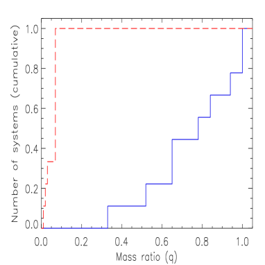
Figure 3: The cumulative distribution of: the observed binary mass ratio (solid line) and the mass ratio distribution predicted by random sampling of the IMF, from Kroupa (2001) (long dashed line).

We assess how different the two distributions are using the one sample Kolmogorov–Smirnov (KS) Test. According to the KS test the scenario that the secondary mass is randomly selected from the IMF may be rejected with almost 100 per cent confidence. Thus it appears the mass ratio distribution of the binary systems is almost certainly not determined by random sampling from the IMF. Clearly, this finding only retains its statistical significance if we can detect all mass ratios equally well. However, the lowest detectable mass is, on average, $\rm{\sim 0.9M_{\rm{\odot}}}$. This is as the sensitivity of spectroastrometry is limited by the relative brightness of binary components. If the primary component of a binary system is more than 5 magnitudes brighter than the secondary the system will probably not be detected by spectroastrometry. As a result the lowest detectable mass ratio is $\rm{\sim 0.3}$, greater than the location of the peak of the mass ratio distribution predicted. Therefore, it is possible that a large number of low mass ratio systems are undetected, which would introduce a bias to the mass ratio observed, skewing the distribution to high values.

To quantify the effect this may have, we consider the case in which this bias has the largest effect possible. We assume every star that is a non detection is a binary system which we do not detect, due to a large difference in brightness between the two components. We assign each fictional system a mass ratio determined by the IMF, which is generally 0.1 and below our detection limits, and add these systems to our sample. Using the KS test we find that the hypothesis that the new ‘observed’ mass ratio originates from randomly sampling the secondary mass from the IMF may still be rejected with 99.55 per cent confidence. In this case the observed mass ratio distribution appears incompatible with the secondary mass being selected at random from the IMF at almost a $\rm 3\sigma$ level. Therefore, the result appears robust, despite our detection limit.

5 Discussion

5.1 On the large FWHM features unaccompanied by positional features

Many stars in the sample, such as AB Aur, present spectroastrometric signatures in which the FWHM features are much more prominent than any positional excursions. Baines et al. (2006) suggest that these features are due to wide binary systems, where wide refers to a separation greater than half the slit width. In the case of AB Aur we detect a similar spectroastrometric signature over H$\rm\alpha$ to Baines et al. (2006). However, a ‘wide’ binary would be resolved in the data, as we use a slit of 5 arcsec. The longslit spectra were visually checked for evidence of a resolved companion, none was found. Therefore, as a resolved system does not create a spectroastrometric signature, there must be another, as yet unconsidered, source of the spectroastrometric signature. It is plausible that light from nebulosity could have distorted the spectroastrometric signatures. Extended emission is noticeable in many longslit spectra. However, it was found that masking the nebulosity had no effect on the spectroastrometric signature observed.

As an alternate explanation we consider the suggestion of Monnier et al. (2006) that some spectroastrometric features could be caused by the presence of dusty halos around HAe/Be stars. Monnier et al. (2006) found that many HAe/Be stars, including AB Aur, are surround by extended features of up to $\rm 0.5$ arcsec. These features contribute up to 20 per cent of the NIR flux detected. Such halos are not well studied, but could constitute light scattered from the remnant natal envelopes of such stars, dust entrained in a wind or localised thermal emission a few au from the central star (Monnier et al., 2006). Such extended emission would be unresolved in a longslit spectrum, and could lead to an increase in the FWHM while not changing the photo-centre position. However, this requires that the line profile of the scattered light is different from the original emission source profile. As discussed by Monnier et al. (2006) this is certainly plausible. A non-uniform distribution of H$\rm\alpha$ flux and line of sight dependent absorption would both result in the observer and the scattering media seeing slightly different line profiles.

We explore whether an unresolved, extended halo could result in a spectroastrometric signature, similar to that observed over the H$\rm\alpha$ line in the case of AB Aur and other stars, using a simple model. The model treats a single star as a point source and surrounds the star with a halo which contributes 20 per cent of the total flux. Here the halo is offset from the central star position by approximately $\rm 0.50$ arcsec. The flux emanating from the halo has a uniform distribution in space. A P-Cygni type profile is assigned to the star and a similar line profile, minus the blue-shifted absorption component and with a slightly different line to continuum ratio, assigned to the halo flux. The total flux distribution is mapped onto an array representing a CCD chip. The array is then convolved with a Gaussian in the spatial direction to represent the effects of seeing. Finally, the output spectrum is extracted in a standard fashion and spectroastrometry is conducted on the artificial observation. We present the results of this exercise in Fig. 4.

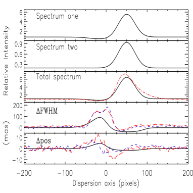
Figure 4: The input spectra, the resultant spectrum and the spectroastrometric signature of the model comprising a star surrounded by a halo. The halo is modelled as a uniform ring from $\rm{0.45}$ arcsec to $\rm{0.60}$ arcsec, centred on a point $\rm{0.075}$ arcsec offset from the star. The seeing used was $\rm 1$ arcsec and the halo contributes 20 per cent of the total flux. The long dashed lines are the spectroastrometric signature of AB Aur over the H$\rm\alpha$ line, in the North-South direction and the short dashed lines are the spectroastrometric signature of AB Aur in the East-West direction. The dot-dashed line is the averaged spectrum of AB Aur in the H$\rm\alpha$ region (the AB Aur data has been rescaled in the dispersion direction).

There exists a qualitative similarity between the model and observed signatures (Fig. 4). The model did not completely recreate the extent of the FWHM feature observed in the case of AB Aur. However, given the unknowns involved, e.g. the amount of light scattered and the extent of the halo, this does not exclude this scenario. Therefore, we conclude that it is likely that FWHM features accompanied by small or nonexistent positional signatures are due, at least in part to unresolved, extended, halos. Alternatively, a wind could also result in a similar positional spectroastrometric signature, see Azevedo et al. (2007). This has important implications on splitting the binary spectra, which are discussed in Section 5.2. We note that some known binary systems exhibited larger FWHM features than positional features, and as such this is not a unique diagnostic.

5.2 An evaluation of the method of Porter et al. (2004)

Implicit in both methods of splitting spectra is the assumption that the system in question comprises of two point sources. In Section 5.1 we demonstrate that dusty halos, which surround some HAe/Be stars (Leinert et al., 2001; Monnier et al., 2006), can give rise to spectroastrometric signatures. It may be expected that if the spectroastrometric signature of a binary system is contaminated by the signature of a halo, the spectra splitting method of Porter et al. (2004) will not be able to correctly separate the constituent spectra. In many situations the method of Porter et al. (2004) failed to fit the observed FWHM spectrum of a known binary system, even when the separation considered was increased to many times the binary separation. Here we investigate whether this could be due to contamination of the binary spectroastrometric signature by an additional, unresolved source of flux.

We construct a model of a binary system with a separation of 0.3 arcsec. The binary system has a difference in brightness of 3.5 magnitudes and is surrounded by a halo that extends from $\rm 0.4$ arcsec to $\rm 0.6$ arcsec from the central star. An artificial longslit spectra is generated and spectroastrometry is applied to the synthetic data to generate the observables necessary to separate the constituent spectra. Finally, the method of Porter et al. (2004) is used to attempt to split the unresolved binary spectrum into its constituent spectra.

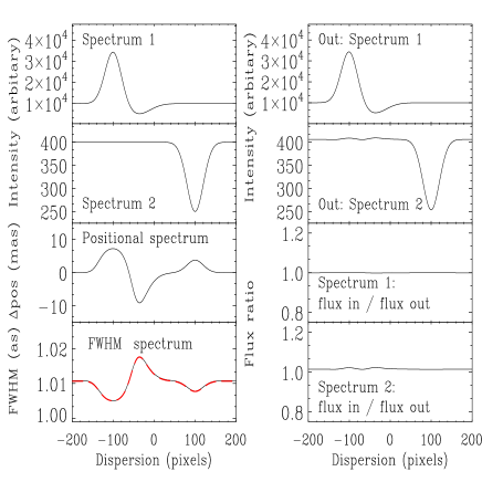
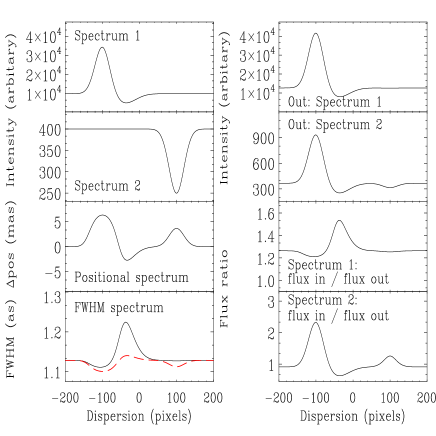
Figure 5: The results of splitting the spectra of the model of a binary system (leftmost two panels) and the model of the same binary system plus an unresolved halo which contributes 20 per cent of the system flux (rightmost two panels). In the panels presenting the observed $\rm\sigma$ distribution the solid line is the observed quantity while the dashed line is the best fit $\rm\sigma$ distribution predicted by the method of Porter et al. (2004).

The results of first modelling the aforementioned binary system without an extended halo component, and the results of including an extended halo component, are displayed in Fig. 5. When no halo component is added the two spectra are clearly separated, demonstrating the power of this approach. The method of Porter et al. (2004) fits the observed FWHM spectrum, and as a consequence splits the binary spectra correctly. In contrast, when the halo component is added to the binary model, the method of Porter et al. (2004) can no longer correctly separate the constituent spectra. The method of Porter et al. (2004) no longer fits the observed FWHM signature, as shown, and consequently fails to separate the two binary spectra correctly. This is only to be expected as: a) the positional and FWHM features observed are no longer due to two point sources and b) the method attempts to apportion the observed flux, which is due to three sources, to only two sources.

This would also be the case if the spectroastrometric signature observed were due to a triple system. The degree to which a third component would compromise the spectra splitting procedure would depend on the relative brightness of the system components. For example, the least bright component would have to be brighter than 1 per cent of the combined flux emanating from the two brightest components to contaminate the spectroastrometric signature. A triple system might be expected to exhibit distinctly different spectroastrometric signatures over different lines. The norm for this sample is for the spectroastrometric signatures over different lines to be consistent, as demonstrated by the example of GU CMa (Fig. 1). Therefore, if triple systems are present in the sample it would appear that the tertiary components are not bright enough to significantly effect the spectroastrometric signatures observed.

In summary, the method of Porter et al. (2004) is compromised if an additional source of flux, besides the binary system, is present. Such a source may a tertiary stellar component, a dusty halo, or material in a wind. We suggest that this is the reason that, more times than not, the method of Porter et al. (2004) clearly does not fit the observed FWHM features and, as a consequence, fails to separate the spectra of many unresolved binary systems. If this is the case for the systems where we apply the spectra splitting procedure, the returned spectra will not be correctly separated. However, we only present separated spectra for systems whose spectroastrometric signature appears solely due to a binary system, with none of the complications mentioned above (see Section 4.1 for the condition used to exclude contaminated signatures).

5.3 On the separation of HAe/Be binary systems

The previously detected systems in the sample have physical separations between $\rm{\sim 40}$ and $\rm{1200}$ au. Unfortunately, this cannot be easily translated into a separation distribution as the stars are at very different distances (between 143 and 2000 pc), and also due to the various selection effects in different detection methods. Of the newly discovered binaries the angular separation to which we are sensitive is in the range $\rm{0.1}$ – $\rm{2.0}$ arcsec. However, the different distances to each star change the physical separation to which this corresponds. For the nearest system at 143 pc, the separation range is 14 – 285 au. For a system at the average distance of a star at 600 pc it is $\rm{\sim}$60 – 1000 au. For the most distant system at 2000 pc, it is 200 – 4000 au.

None of the previously detected binaries are closer than 30 au, which is the peak of the field G-dwarf distribution. Half of all G-dwarf binary systems have separations less than 30 au (Duquennoy & Mayor, 1991). Of the newly discovered binaries, only one could be closer than 30 au (V1366 Cas at 164 pc), and two other systems could have separations as small as 30 – 40 au. Therefore, at least 60 per cent of HAe/Be stars have a companion between about 30 – 4000 au, and probably in the range 60 – 1000 au. This is significantly greater than the fraction of G-dwarfs at the same separations (around 40 per cent between 30 – 4000 au, and 25 per cent between 60 – 1000  au). This overabundance of binaries is not dissimilar to, but apparently larger than, the overabundance of binary systems found in young T Tauri stars (see Duchêne et al. (2007) and references therein).

Thus, unless there is an almost complete lack of companions $\rm{<30}$ au, it is difficult to imagine that the binary fraction of HAe/Be stars is much less than 100 per cent. If HAe/Be stars exhibit a similar abundance of companions $\rm{<30}$ au to G-dwarfs this would suggest that many HAe/Be stars are triple or higher-order systems. Indeed we present the detection of four additional components in previously detected binary systems, meaning that these systems are at least triple systems.

It is worth noting that many of these systems are relatively soft, with separations greater than a few hundred au. As a result, these systems are susceptible to destruction in dense clusters (see Parker et al. (2009) and references therein). This suggests that many of these HAe/Be stars have not spent a significant time in a very dense environments, e.g. densities of $>10^{4}$ M_⊙ pc^-3, which are not unusual in star forming regions of young clusters. Indeed, Testi et al. (1999) found that no Herbig Ae stars are associated with clustered environments, and that while Herbig Be stars are sometimes situated in a small cluster, the associated stellar densities are approximately $\rm{10^{2}-10^{3}pc^{-3}}$.

5.4 The mass ratio and formation mechanisms of HAe/Be binary systems

It appears that the mass ratio of Herbig Ae/Be binary systems is skewed towards relatively high values, and is inconsistent with random sampling from the IMF. However, as the spectra splitting technique did not work in every case, the sample size is too small to attempt to constrain the underlying distribution of mass ratios. Instead, we discuss the possible implications this finding has on the formation mechanisms of intermediate mass stars. We note that random pairing of binary components has already been excluded in the OB association Sco OB2 (Kouwenhoven et al., 2005). Here we extend this finding to younger systems, and higher masses.

Baines et al. (2006) found that the circumstellar discs of the components of Herbig Ae/Be systems are preferentially aligned with the binary position angle. This already suggests that the secondary formed by disc fragmentation, see Goodwin et al. (2007). As noted by Kouwenhoven et al. (2009), disc fragmentation would be expected to produce stars of roughly similar mass (within a factor of a few). Disc fragmentation should occur during the earliest phases of star formation. During such phases there is an abundance of gas to accrete, and the circumprimary disc is still massive enough to fragment. The secondary in the disc is able to accrete material from the disk more easily than the primary, as the angular momentum of the material is closer to the secondary than the primary (Whitworth et al., 1995; Bate & Bonnell, 1997). Therefore, this scenario results in a binary system with a high mass ratio, higher than if random sampling from the IMF determined the mass of the secondary. Indeed, recent models of massive star formation demonstrate that binary systems with high mass ratios (0.7) and large separations ($\rm\sim 1000$ au) can be formed from disk fragmentation (Krumholz et al., 2009).

The separations of the binary systems in our sample also suggest disc fragmentation as the mode of binary formation. Whitworth & Stamatellos (2006) show that a massive disc can fragment beyond a critical radius $R_{\rm frag}$ which depends on the mass of the primary $M_{\star}$ as follows:

$$R_{\rm{frag}}>150\left(\frac{M_{\rm{\star}}}{\rm{M_{\odot}}}\right)^{1/3}\,\,\,\,{\rm{au}}$$

For a Herbig Ae/Be star $M_{\star}\sim 10M_{\odot}$, and so $R_{\rm frag}>300$ au, which is a typical separation of the systems in our sample.

Therefore, the properties of the Herbig Ae/Be binary systems observed indicate that these systems formed via disk fragmentation. Given that the sample includes stars as massive as $\mathrm{\sim 15M_{\odot}}$, this favours the core collapse and subsequent monolithic accretion scenario of massive star formation (Krumholz et al., 2009), as opposed to the merger and capture scenarios (Bally & Zinnecker, 2005; Moeckel & Bally, 2007).

The Herbig Ae/Be stars in this sample are not located in dense clusters (Testi et al., 1999). In addition, the wide separations of the binary systems and their young ages suggest that they formed in isolation. Firstly, binaries this wide are relatively soft and could not have spent a significant amount of time in a dense cluster, see Parker et al. (2009). Secondly, no binary this wide could have survived ejection from a cluster. Together this suggests that a fairly large core ($\rm{>10M_{\odot}}$) formed in relative isolation and produced a massive binary system, rather than a small cluster. That these HAe/Be stars formed in a massive, isolated core shows that competitive accretion, e.g. Bonnell et al. (1998), is not required to form stars of up to at least $\rm{10M_{\odot}}$, as presumably no larger reservoir of gas existed beyond the single core.

This cannot be infrequent as we find several Herbig Ae/Be systems which fit this pattern. However, the sample we have used is not complete, the population of HAe/Be is heterogeneous to begin with and the selection criteria may well impose certain selection effects on membership of the HAe/Be class. Biases and incompleteness are impossible to fully quantify, but we can state that a not insignificant fraction of A/B stars can form in isolation from a massive core. This is in qualitative agreement with de Wit et al. (2005), who report that even O type stars may form in isolation. In addition, Parker & Goodwin (2007) also find that a few per cent of massive stars might form in relative isolation.

6 Conclusions

In this paper we present spectroastrometric observations of a relatively large sample of HAe/Be stars. Here we present the salient findings of this work:

• We find a high binary fraction, $\rm{74\pm 6}~{}percent$, consistent with previous studies.

• Using spectroastrometry to separate the unresolved binary spectra we determine spectral types for the components of 9 systems.

• The mass ratios of these systems, determined from the constituent spectral types, are inconsistent with a secondary mass randomly selected from the IMF.

• Although our sample is small this result constrains the mode of binary formation in that the mass ratios and separations of the binary systems observed suggest that the secondary forms via disk fragmentation.

• The properties of the binary systems observed indicate that these systems have not spent a significant amount of time in dense, clustered environments. Therefore, these systems demonstrate that isolated star formation can produce stars as massive as $\rm{\sim 10-15M_{\odot}}$.

Appendix A A summary of the spectroastrometric signatures

In Table 5 we present a summary of the spectroastrometric signatures over the H$\rm\alpha$ or H$\rm\beta$ lines for the 47 stars in the sample. Where possible the signature over H$\alpha$ is summarised. However, not all the objects in the sample were observed in the $R$ band. Therefore, in these cases the properties of the H$\beta$ signature are presented.

Table 5: A summary of the spectroastrometric results across $\rm H\alpha$ or H$\mathrm{\beta}$. Column 1 lists the objects observed, columns 2 and 3 contain the continuum uncertainty in the position and FWHM spectra respectively, column 4 lists the average equivalent width of the line in question (accurate to 10% on average), column 5 denotes the emission profile type while columns 6 and 7 list the observed change in centroid position and FWHM over the line, and column 8 contains the calculated PA of the systems detected.

Object	$\overline{\rm{pos\;\sigma}}\,$	$\rm{\overline{FWHM\;\sigma}}$	$\overline{\rm H\alpha\;W_{\lambda}}$	$\rm H\alpha$ $\rm{profile^{{\dagger}}}$	$\rm\Delta pos\,\,\,\,$	$\rm\Delta$FWHM	PA
	(mas)	(mas)	$\rm(\AA)$		(mas)	(mas)	$\rm({\circ})$
VX Cas (WHT)	1.2	3.0	$-$1.7	IIR	$\rm{Artifact^{{\ddagger}}}$	97 $\rm{\pm}$ 3
VX Cas (INT)	3.0	6.8	$\rm-1.8$	IIR	Artifact	61 $\rm{\pm}$ 7
IP Per	1.8	4.4	$\rm 2.8$	M	$\mathrm{\leq}$8	15 $\rm{\pm}$ 5
AB Aur	1.2	2.6	$-$22	IVB	14 $\rm\pm$ 1	233 $\rm\pm$ 3	45.8 $\rm\pm$ 5.1
MWC 480	1.1	2.9	$-$18	IVB	$\mathrm{\leq}$4	145 $\rm\pm$ 3
UX Ori	1.7	4.0	3.0	IIR	Artifact	134 $\rm\pm$ 4
HD 35929	0.9	3.6	1.8	I	Artifact	13 $\rm\pm$ 3
V380 Ori	1.9	5.3	$\rm-93$	I	$\rm 37\pm 2$	74 $\rm\pm$ 7	264.8 $\rm\pm$ 2.4
MWC 758	1.0	2.3	$-$6.3	I	$\mathrm{\leq}$4	21 $\rm\pm$ 2
HD 244604	4.1	11	1.6	IVB	Artifact	80 $\rm\pm$ 11
HD 37357	1.3	2.9	$\rm 0.7$	IIIB	$\rm 50\pm 1$	45 $\rm{\pm}$ 3	234.9$\rm\pm$ 1.0
MWC 120 (WHT)	1.3	3.2	$-$28	IIIB	Artifact	154 $\rm\pm$ 3
MWC 120 (INT)	1.1	2.7	$\rm-28$	IIB	$\rm 25\pm 1$	123 $\rm\pm$ 3	33.7 $\rm\pm$ 1.5
MWC 137	4.4	11	$\rm-665$	I	Artifact	94 $\rm\pm$ 12
HD 45677	1.5	4.0	$-$235	IIB	Artifact	59 $\rm\pm$ 4
LkH$\rm\alpha$ 215	2.3	5.1	$\rm-30$	IIR	$\rm 25\pm 3$	220 $\rm\pm$ 5	230.7 $\rm\pm$ 6.0
MWC 147	1.3	3.2	$-$71	II	Artifact	50 $\rm\pm$ 3
R Mon	7.8	22	$\rm-91$	IIIB	$\rm 160\pm 8$	Artifact	279.3 $\rm\pm$ 3.7
V742 Mon	1.0	2.0	$\rm-43$	I	$\rm 76\pm 1$	204 $\rm\pm$ 2	47.0 $\rm\pm$ 0.4
GU CMa	1.4	2.9	$-$10	I	144 $\rm\pm$ 1	101 $\rm\pm$ 3	197.9 $\rm\pm$ 0.2
MWC 166	1.9	4.8	1.3	Ab	49 $\rm\pm$ 2	29 $\rm\pm$ 5	298.3 $\rm\pm$ 0.7
HD 76868	0.9	3.3	$\rm-11$	I	$\rm 33\pm 1$	100 $\rm\pm$ 4	51.4 $\rm\pm$ 1.1
MWC 297	2.0	4.9	$-$537	I	Artifact	34 $\rm\pm$ 6
HD 179218	1.5	3.6	$-$3.5	M	$\mathrm{\leq}$5	$\mathrm{\leq}$12
HD 190073	1.2	2.9	$-$27	IVB	Artifact	108 $\rm\pm$ 3
BD +40 4124	3.0	8.4	$-$147	IIB	9 $\rm\pm$ 3	89 $\rm\pm$ 8	$\sim$0
$\rm{MWC\,361_{({2.5^{\prime\prime}}{slit})}}$	0.9	2.4	$-$62	II	Artifact	35 $\rm\pm$ 2
$\rm{MWC\,361_{({4^{\prime\prime}}{slit})}}$	0.9	2.6	$-$62	II	Artifact	43 $\rm\pm$ 3
Il Cep	0.7	2.4	$-$18	I	11 $\rm\pm$ 1	49 $\rm\pm$ 2	234.3 $\rm\pm$ 2.0
BHJ 71	2.7	7.0	$-$58	IIR	Artifact	61 $\rm\pm$ 7
MWC 1080	1.9	4.8	$-$112	IVB	109 $\rm\pm$ 2	586 $\rm\pm$ 5	269.2 $\rm\pm$ 1.5
Object	$\overline{\rm{pos\;\sigma}}\,$	$\rm{\overline{FWHM\;\sigma}}$	$\overline{\rm H\beta\;W_{\lambda}}$	$\rm H\beta$ $\rm{profile^{{\dagger}}}$	$\rm\Delta pos\,\,\,\,$	$\rm\Delta$FWHM	PA
	(mas)	(mas)	$\rm(\AA)$		(mas)	(mas)	$\rm({\circ})$
V594 Cas	1.6	3.3	$\rm{-4.2}$	IVB	Artifact	$\rm{233\pm 4}$
V1185 Tau	1.8	4.2	16	Ab	$\mathrm{\leq}$8	$\mathrm{\leq}$19
V1012 Ori	3.3	8.3	9.5	Ab	Artifact	$\rm{256\pm 8}$
V1366 Ori	1.3	2.8	18	Ab	Artifact	$\rm{25\pm 2}$
V346 Ori	1.3	3.8	14	Ab	Artifact	$\rm{39\pm 4}$
HK Ori	5.0	10	$\rm{-0.7}$	IIIB	$\mathrm{40\pm 5}$	$\rm{135\pm 10}$	$\mathrm{46.9\pm 3.1}$
V1271 Ori	1.6	3.5	14	IIB	$\mathrm{\leq}$5	$\rm{40\pm 3}$
T Ori	1.8	4.1	14	Ab	$\mathrm{47\pm 2}$	$\rm{117\pm 4}$	$\mathrm{107.2\pm 2.5}$
V586 Ori	2.5	5.8	16	Ab	$\mathrm{55\pm 3}$	$\rm{246\pm 6}$	$\mathrm{216.8\pm 3.3}$
V1788 Ori	1.9	4.7	18	Ab	$\mathrm{65\pm 2}$	$\rm{114\pm 4}$	$\mathrm{131.3\pm 6.6}$
HD 245906	2.3	6.1	12	Ab	$\mathrm{24\pm 3}$	$\rm{39\pm 6}$	$\mathrm{81.9\pm 3.1}$
RR Tau	3.8	8.6	6.7	IIR	$\mathrm{21\pm 4}$	$\rm{187\pm 8}$
V350 Ori	2.0	4.8	17	Ab	Artifact	$\rm{124\pm 5}$
MWC 790	10	28	$\rm{-23}$	I	$\mathrm{\leq}$44	$\rm{191\pm 26}$
V590 Mon	4.6	12	4.5	IIB	$\mathrm{\leq}$20	$\mathrm{\leq}$45
OY Gem	3.2	8.3	$\rm{-100}$	I	$\mathrm{27\pm 3}$	$\rm{215\pm 9}$	$\mathrm{157.5\pm 8.0}$
HD 81357	0.6	2.1	6.5	IIR	Artifact	$\rm{47\pm 2}$
SV Cep	1.9	4.3	15	Ab	Artifact	$\rm{111\pm 5}$
MWC 655	1.4	3.3	$\rm{-0.3}$	II	$\mathrm{\leq}$6	$\mathrm{\leq}$14

Appendix B Hi spectroastrometric signatures

In Fig. 6 the H$\rm\alpha$ or H$\rm\beta$ profiles and the associated spectroastrometric signatures of the 47 stars in the sample are presented. For each object the average, normalised, intensity spectrum is presented alongside the position spectra in the two perpendicular directions observed. In addition, we also present the FWHM spectra, also in these two directions. To keep the appendix concise only one profile per observation is presented, where possible the H$\alpha$ signature, and where not the H$\beta$ signature. Artifacts are indicated by dashed lines.

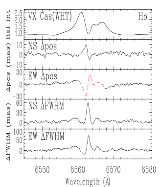
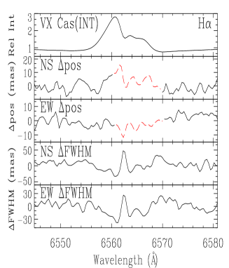
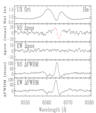
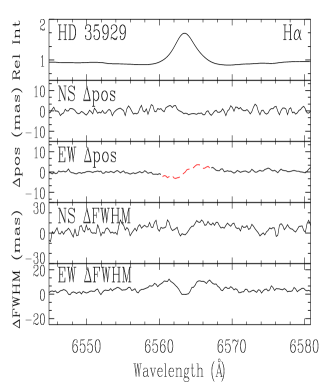
Figure 6: H$\rm\alpha$ profiles and spectroastrometric signatures. From left to right: VX Cas (data from the WHT), VX Cas (data from the INT), IP Per, AB Aur, MWC 480, UX Ori, HD 35929, V380 Ori and MWC 708.

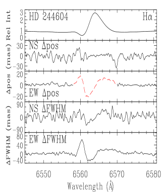
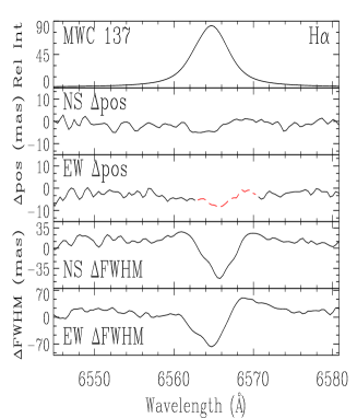
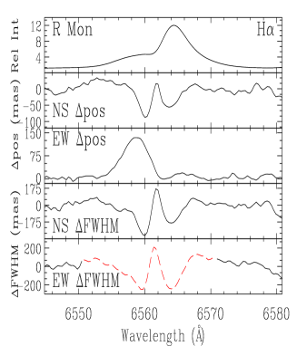
Figure 6: H$\rm\alpha$ profiles and spectroastrometric signatures. From left to right: HD 244604, HD 37357, MWC 120 (data from the WHT), MWC 120 (data from the INT), MWC 137, HD 45677, LkH$\mathrm{\alpha}$ 215, MWC 147 (data from the WHT) and R Mon.

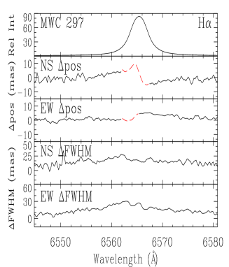
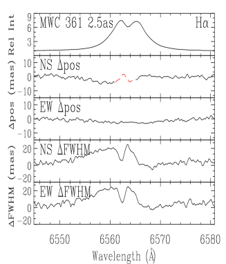
Figure 6: H$\rm\alpha$ profiles and spectroastrometric signatures. From left to right: V742 Mon, GU CMa (data from the WHT), MWC 166, HD 76868, MWC 297, HD 179218, HD 190073, BD+40 4124 and MWC 361 (data obtained with a $\mathrm{2.5}$ arcsec slit).

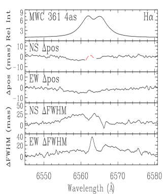
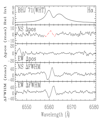
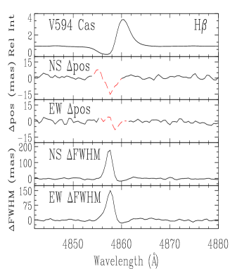
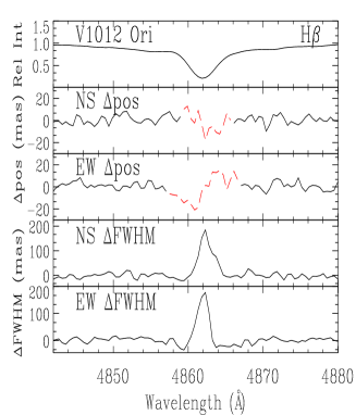
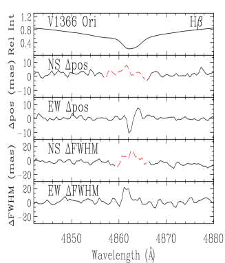
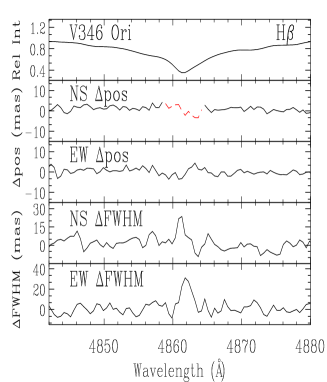
Figure 6: H$\rm\alpha$ and H$\rm\beta$ profiles and spectroastrometric signatures. From left to right: MWC 361 (data obtained with a $\mathrm{4}$ arcsec slit), Il Cep, BHJ 71 (data from the WHT), MWC 1080, V594 Cas, V1185 Tau, V1012 Ori, V1366 Ori and V346 Ori.

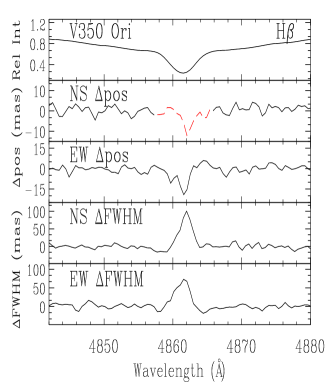
Figure 6: H$\rm\beta$ profiles and spectroastrometric signatures. From left to right: HK Ori, V1271 Ori, T Ori, V586 Ori, V1788 Ori, HD 245906, RR Tau, V350 Ori and MWC 790.

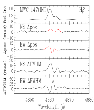
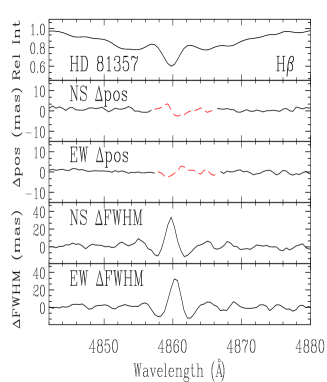
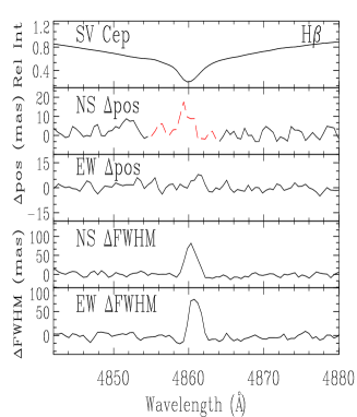
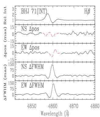
Figure 6: H$\rm\beta$ profiles and spectroastrometric signatures. From left to right: MWC 147 (data from the INT), V590 Mon, OY Gem, GU CMa (data from the INT), HD 81357, SV Cep, MWC 655 and BHJ 71 (data from the INT).

References

- Azevedo et al. (2007) Azevedo R., Folha D. F. M., Gameiro J. F., Calvet N., 2007, ApJ, 670, 1234
- Bailey (1998a) Bailey J. A., 1998a, Proc. SPIE, 3555, 932
- Bailey (1998b) Bailey J., 1998b, MNRAS, 301, 161
- Baines et al. (2006) Baines D., Oudmaijer R. D., Porter J. M., Pozzo M., 2006, MNRAS, 367, 737
- Bally & Zinnecker (2005) Bally J., Zinnecker H., 2005, AJ, 129, 2281
- Bate & Bonnell (1997) Bate M. R., Bonnell I. A., 1997, MNRAS, 285, 33
- Bertout et al. (1999) Bertout C., Robichon N., Arenou F., 1999, A&A, 352, 574
- Bidelman (1954) Bidelman W. P., 1954, ApJS, 1, 175
- Bonnell et al. (1998) Bonnell I. A., Bate M. R., Zinnecker H., 1998, MNRAS, 298, 93
- Bouvier et al. (2007) Bouvier J., Alencar S. H. P., Harries T. J., Johns-Krull C. M., Romanova M. M., 2007, in Reipurth B., Jewitt D., Keil K., eds, Protostars and Planets V, p. 479
- Bouvier & Corporon (2001) Bouvier J., Corporon P., 2001, in Zinnecker H., Mathieu R., eds, Proc. IAU Symp. 55, The Formation of Binary Stars, p. 200,
- Brannigan et al. (2006) Brannigan E., Takami M., Chrysostomou A., Bailey J., 2006, MNRAS, 367, 315
- Carmona et al. (2007) Carmona A., van den Ancker M. E., Henning T., 2007, A&A, 464, 687
- de Wit et al. (2005) de Wit W. J., Testi L., Palla F., Zinnecker H., 2005, A&A, 437, 247
- Duchêne et al. (2007) Duchêne G., Delgado-Donate E., Haisch Jr. K. E., Loinard L., Rodríguez L. F., 2007, in Reipurth B., Jewitt D., Keil K., eds, Protostars and Planets V, p. 379
- Duquennoy & Mayor (1991) Duquennoy A., Mayor M., 1991, A&A, 248, 485
- Fabricius & Makarov (2000) Fabricius C., Makarov V. V., 2000, A&A, 356, 141
- Fu et al. (1997) Fu H.-H., Hartkopf W. I., Mason B. D., McAlister H. A., Dombrowski E. G., Westin T., Franz O. G., 1997, AJ, 114, 1623
- Fuente et al. (2006) Fuente A., Alonso-Albi T., Bachiller R., Natta A., Testi L., Neri R., Planesas P., 2006, ApJ, 649, L119
- Ghez et al. (1993) Ghez A. M., Neugebauer G., Matthews K., 1993, AJ, 106, 2005
- Goodwin et al. (2007) Goodwin S. P., Kroupa P., Goodman A., Burkert A., 2007, in Reipurth B., Jewitt D., Keil K., eds, Protostars and Planets V, p. 133
- Grady (2007) Grady C. A. et al., 2007, ApJ, 665, 1391
- Guetter (1968) Guetter H. H., 1968, PASP, 80, 197
- Harmanec (1988) Harmanec P., 1988, Bull. Astron. Inst. Czechoslovakia, 39, 329
- Hartkopf et al. (1996) Hartkopf W. I., Mason B. D., McAlister H. A., Turner N. H., Barry D. J., Franz O. G., Prieto C. M., 1996, AJ, 111, 936
- Herbig (1960) Herbig G. H., 1960, ApJS, 4, 337
- Herbig & Bell (1988) Herbig G. H., Bell K. R., 1988, Lick Obs. Bull.
- Hernández et al. (2004) Hernández J., Calvet N., Briceño C., Hartmann L., Berlind P., 2004, AJ, 127, 1682
- Hiltner (1956) Hiltner W. A., 1956, ApJS, 2, 389
- Hubrig et al. (2007) Hubrig S., Marco O., Stelzer B., Schöller M., Huélamo N., 2007, MNRAS, 381, 1569
- Kahn (1974) Kahn F. D., 1974, A&A, 37, 149
- Kouwenhoven et al. (2005) Kouwenhoven M. B. N., Brown A. G. A., Zinnecker H., Kaper L., Portegies Zwart S. F., 2005, A&A, 430, 137
- Kouwenhoven et al. (2009) Kouwenhoven M. B. N., Brown A. G. A., Goodwin S. P., Portegies Zwart S. F., Kaper L., 2009, A&A, 493, 979
- Kraus et al. (2008) Kraus S., Preibisch T., Ohnaka K., 2008, ApJ, 676, 490
- Kroupa (2001) Kroupa P., 2001, MNRAS, 322, 231
- Kroupa & Burkert (2001) Kroupa P., Burkert A., 2001, ApJ, 555, 945
- Krumholz et al. (2009) Krumholz M. R., Klein R. I., McKee C. F., Offner S. S. R., Cunningham A. J., 2009, Sci, 323, 754
- Larson & Starrfield (1971) Larson R. B., Starrfield S., 1971, A&A, 13, 190
- Leinert et al. (2001) Leinert C., Haas M., Ábrahám P., Richichi A., 2001, A&A, 375, 927
- Leinert et al. (1997) Leinert C., Richichi A., Haas M., 1997, A&A, 318, 472
- Mannings & Sargent (1997) Mannings V., Sargent A. I., 1997, ApJ, 490, 792
- Moeckel & Bally (2007) Moeckel N., Bally J., 2007, ApJ, 656, 275
- Monnier et al. (2006) Monnier J. D., Berger J.-P., Millan-Gabet R. et al., 2006, ApJ, 647, 444
- Mora et al. (2004) Mora A., Eiroa C., Natta A. et al., 2004, A&A, 419, 225
- Mora et al. (2001) Mora A., Merín B., Solano E. et al., 2001, A&A, 378, 116
- Mottram et al. (2007) Mottram J. C., Vink J. S., Oudmaijer R. D., Patel M., 2007, MNRAS, 377, 1363
- Parker & Goodwin (2007) Parker R. J., Goodwin S. P., 2007, MNRAS, 380, 1271
- Parker et al. (2009) Parker R. J., Goodwin S. P., Kroupa P., Kouwenhoven M. B. N., 2009, MNRAS, 397, 1577
- Patel et al. (2005) Patel N. A., Curiel S., Sridharan T. K. et al., 2005, Nat, 437, 109
- Pirzkal et al. (1997) Pirzkal N., Spillar E. J., Dyck H. M., 1997, ApJ, 481, 392
- Porter et al. (2004) Porter J. M., Oudmaijer R. D., Baines D., 2004, A&A, 428, 327
- Preibisch et al. (1999) Preibisch T., Balega Y., Hofmann K.-H., Weigelt G., Zinnecker H., 1999, New Astron., 4, 531
- Reipurth et al. (1996) Reipurth B., Pedrosa A., Lago M. T. V. T., 1996, A&AS, 120, 229
- Reipurth & Zinnecker (1993) Reipurth B., Zinnecker H., 1993, A&A, 278, 81
- Rodgers et al. (2002) Rodgers B., Wooden D. H., Grinin V., Shakhovsky D., Natta A., 2002, ApJ, 564, 405
- Shevchenko & Vitrichenko (1994) Shevchenko V. S., Vitrichenko E. A., 1994, in The P. S., Perez M. R., van den Heuvel E. P. J., eds, ASP Conf. Ser. Vol. 62, The Nature and Evolutionary Status of Herbig Ae/Be Stars, p. 55
- Smith et al. (2005) Smith K. W., Balega Y. Y., Duschl W. J., Hofmann K.-H., Lachaume R., Preibisch T., Schertl D., Weigelt G., 2005, A&A, 431, 307
- Smith (1972) Smith M. A., 1972, ApJ, 175, 765
- Takami et al. (2003) Takami M., Bailey J., Chrysostomou A., 2003, A&A, 397, 675
- Takami et al. (2001) Takami M., Bailey J., Gledhill T. M., Chrysostomou A., Hough J. H., 2001, MNRAS, 323, 177
- Testi et al. (1999) Testi L., Palla F., Natta A., 1999, A&A, 342, 515
- Thé et al. (1994) Thé P. S., de Winter D., Perez M. R., 1994, A&AS, 104, 315
- Thomas et al. (2007) Thomas S. J., van der Bliek N. S., Rodgers B., Doppmann G., Bouvier J., 2007, in Hartkopf W. I., Guinan E. F., Harmanec P., eds, IAU Symp. 240, Binary Stars as Critical Tools & Tests in Contemporary Astrophysics, p. 250
- Tody (1993) Tody D., 1993, in Hanisch R. J., Brissenden R. J. V., Barnes J., eds, ASP Conf.Ser. Vol. 52, Astronomical Data Analysis Software and Systems II, p. 173
- Turner et al. (2007) Turner N. J., Quataert E., Yorke H. W., 2007, ApJ, 662, 1052
- Vieira et al. (2003) Vieira S. L. A. Corradi W. J. B., Alencar S. H. P., Mendes L. T. S., Torres C. A. O., Quast G. R., Guimarães M. M., da Silva L., 2003, AJ, 126, 2971
- Vink et al. (2002) Vink J. S., Drew J. E., Harries T. J., Oudmaijer R. D., 2002, MNRAS, 337, 356
- Vink et al. (2005a) Vink J. S., Drew J. E., Harries T. J., Oudmaijer R. D., Unruh Y., 2005a, MNRAS, 359, 1049
- Vink et al. (2005b) Vink J. S., O’Neill P. M., Els S. G., Drew J. E., 2005b, A&A, 438, L21
- Weigelt et al. (2002) Weigelt G., Balega Y. Y., Hofmann K.-H., Preibisch T., 2002, A&A, 392, 937
- Wheelwright et al. (2009) Wheelwright H. E., Oudmaijer R. D., Schnerr R. S., 2009, A&A, 497, 487
- Whitworth et al. (1995) Whitworth A. P., Chapman S. J., Bhattal A. S., Disney M. J., Pongracic H., Turner J. A., 1995, MNRAS, 277, 727
- Whitworth & Stamatellos (2006) Whitworth A. P., Stamatellos D., 2006, A&A, 458, 817
- Wolf et al. (2001) Wolf S., Stecklum B., Henning T., 2001, in Zinnecker H., Mathieu R., eds, IAU Symp. 200, The Formation of Binary Stars, p. 295
- Yorke & Sonnhalter (2002) Yorke H. W., Sonnhalter C., 2002, ApJ, 569, 846
- Zinnecker & Yorke (2007) Zinnecker H., Yorke H., 2007, ARA&A, 45, 481