Cosmological Implications of 5-dimensional Brans-Dicke Theory

Abstract

The five dimensional Brans-Dicke theory naturally provides two scalar fields by the Killing reduction mechanism. These two scalar fields could account for the accelerated expansion of the universe. We test this model and constrain its parameter by using the type Ia supernova (SN Ia) data. We find that the best fit value of the 5-dimensional Brans-Dicke coupling contant is $\omega=-1.9$. This result is also consistent with other observations such as the baryon acoustic oscillation (BAO).

I Introduction

The expansion of the Universe is shown to be accelerating by the observations of type Ia supernovae (SN Ia) Perlmutter99 ; Riess98 . This is usually attributed to the contribution of an unknown component, dubbed dark energy, which has negative pressure and makes up about three quarters of the total cosmic density (for recent measurements, see e.g. Ref. Komatsu08 ; Gong08 ). The simplest model for dark energy is the cosmological constant (CC), which is consistent with most of the observations today. However, there are two big problems for CC, i.e. the well-known “fine tuning problem” and the “coincidence problem” . As alternatives, and also to solve these two problems, many dynamical dark energy models with scalar field have been proposed, such as quintessence Wetterich88 ; Ratra88 ; FJ97 ; CDS98 ; CLW98 ; Carroll98 ; ZMS99 ; ZMS991 , phantom Caldwell02 , quintomFWZ05 , K-essence Chiba00 ; Armendariz00 , tachyon Padmanabhan02 ; Bagla03 ; Abramo03 ; Agui04 ; Guo04 ; Copeland05 and so on. Nevertheless, in most cases the fundamental physical origin of these scalar fields remain unknown, but just added by hand.

In Ref. Qiang05 , by generalizing the Brans-Dicke theory to five dimensions and exploring its effect on the 4-dimensional world, another interesting approach to explain the cosmic accelerated expansion was proposed. Under the condition that the extra dimension is compact and sufficiently small, a spacelike Killing vector field $\xi^{a}$ arises naturally, in which case the 5D Brans-Dicke theory can be reduced to a 4D theory, such that the 4-metric is coupled with two scalar fields $\phi$ and $\lambda$. Notes that here the scalar fields in four dimension stem naturally from a fundamental theory of gravity. Considering the hypersurface-orthogonal property of $\xi^{a}$, the line element in five dimension can take the form as

$$ds^{2}=g_{\mu\nu}dx^{\mu}dx^{\nu}+\lambda dx^{5}dx^{5},$$ (1)

thus the scalar $\lambda$ also plays the role of a “scale factor” of the extra dimension. It was shown in Ref. Qiang05 that these two scalar fields originated from the Killing reduction of the 5D Brans-Dicke theory may lead to the accelerated expansion of the universe. More detailed analysis is desirable to check if the theory can match the current observational data such as the SN Ia and the baryon acoustic oscillation.

In this paper, we compare the predictions of the cosmic expansion rate of this theory with the current cosmological observations, and constrain the 5D Brans-Dicke theory by means of the SN Ia data and the baryon acoustic oscillation (BAO) measurements. This work is based on the fact that the 4-dimensional gravitational constant $G$ varies extremely slowly with time Turyshev04 in the current epoch. Thus we assume that $G$ is a constant at the “low redshift”, so that the accretion of the white dwarf will not be affected, hence the luminosity and light curve of the observed SN Ia (redshifts range from 0 to 2) are not affected by the slow variations of $G$, and the SN Ia can still be used as the standard candle. Furthermore, if we assume that $G$ is almost a constant throughout the history of the Universe, we could also use the information from the large scale structure (e.g. BAO) to perform the constraints. However, we should note that $G=(\phi\lambda^{1/2}L)^{-1}$ Qiang05 , where $L$ is the coordinate scale of the extra dimension. Although $G$ is almost constant in four dimension, $G^{(5)}\sim\phi^{-1}$ is not necessarily a constant and can still evolve with time.

II theory

The action of the five dimensional Brans-Dicke theory is given by

$$S_{5} = \int d^{5}x\sqrt{-g}(\phi R^{(5)}-\frac{\omega}{\phi}g^{ab}(\nabla_{a}\phi)\nabla_{b}\phi)$$ (2)

$$+16\pi\int d^{5}x\sqrt{-g}L_{m}^{(5)},$$

where $R^{(5)}$ is the curvature scalar of the 5D metric $g_{ab}$, $\phi$ is the scalar field, $\omega$ is the coupling constant, and $L^{(5)}_{m}$ represents the Lagrangian of 5D matter fields. Variation of this action gives the field equations

$$R_{ab}^{(5)}-\frac{1}{2}g_{ab}R^{(5)} = \frac{\omega}{\phi^{2}}((\triangledown_{a}\phi)\triangledown_{b}\phi-\frac{1}{2}g_{ab}(\triangledown^{c}\phi)\triangledown_{c}\phi)$$ (3)

$$+\phi^{-1}(\triangledown_{a}\triangledown_{b}\phi-g_{ab}\triangledown^{c}\triangledown_{c}\phi)$$

$$+8\pi\phi^{-1}T_{ab}^{(5)},$$

$$\triangledown^{a}\triangledown_{a}\phi = 8\pi\frac{T^{(5)}}{4+3\omega},$$ (4)

where $T^{(5)}_{ab}$ represents the 5D energy momentum tensor of matter fields and $T^{(5)}=T^{(5)}_{ab}g^{ab}$.

The topology of the spacetime manifold is assumed to be $\mathbb{R}^{4}\times\mathbb{S}^{1}$, and the extra dimension is confined into extremely small scales Hoyle . Thus a Killing vector field $\xi^{a}$ arises naturally in the low energy regime Blagojevic02 . Considering the case where $\xi^{a}$ is everywhere spacelike and hypersurface orthogonal, the line element can be written down as Eq.(1). The 4D Ricci tensor $R^{(4)}_{ab}$ of the 4-metric $h_{ab}$ and the scalar field $\lambda$ are related to the 5D Ricci tensor $R^{(5)}_{ab}$ by

$$R_{ab}^{(4)}=\frac{1}{2}\lambda^{-1}D_{a}D_{b}\lambda-\frac{1}{4}\lambda^{-2}(D_{a}\lambda)D_{b}\lambda+h_{a}^{c}h_{b}^{d}R_{cd}^{(5)}$$ (5)

and

$$D^{2}\lambda=\frac{1}{2}\lambda^{-1}(D^{a}\lambda)D_{a}\lambda-2R_{ab}^{(5)}\xi^{a}\xi^{b}.$$ (6)

where $D_{a}$ is the covariant derivative operator on the 4D spacetime obtained by Killing reduction

$$D_{e}T^{b\ldots d}_{a\ldots c}=h^{p}_{e}h^{m}_{a}\ldots h^{n}_{c}h^{b}_{r}\ldots h^{d}_{s}\nabla_{p}T^{r\ldots s}_{m\ldots n},$$

and $D^{2}\equiv D^{a}D_{a}$. After the Killing reduction we obtain the 4-dimensional field equations Qiang05 :

$$G_{ab}^{(4)} = 8\pi\phi^{-1}L^{-1}\lambda^{-\frac{1}{2}}T_{ab}^{(4)}+\frac{1}{2}\lambda^{-1}(D_{a}D_{b}\lambda-h_{ab}D^{c}D_{c}\lambda)$$ (7)

$$-\frac{1}{4}\lambda^{-2}((D_{a}\lambda)D_{b}\lambda-h_{ab}(D^{c}\lambda)D_{c}\lambda)$$

$$+\frac{\omega}{\phi^{2}}((D_{a}\phi)D_{b}\phi-\frac{1}{2}h_{ab}(D^{c}\phi)D_{c}\phi)$$

$$+\phi^{-1}(D_{a}D_{b}\phi-h_{ab}D^{c}D_{c}\phi)$$

$$-\frac{\phi^{-1}}{2}\lambda^{-1}h_{ab}(D^{c}\lambda)D_{c}\phi,$$

$$D^{a}D_{a}\lambda = \frac{1}{2}\lambda^{-1}(D^{a}\lambda)D_{a}\lambda-\phi^{-1}(D^{a}\lambda)D_{a}\phi$$ (8)

$$+ \frac{8\pi}{L\lambda^{\frac{1}{2}}\phi}\left(\frac{2\omega+2}{4+3\omega}T^{(4)}-\frac{4\omega+6}{4+3\omega}P\right),$$

and

$$D^{a}D_{a}\phi=-\frac{1}{2}\lambda^{-1}(D^{c}\lambda)D_{c}\phi+\frac{8\pi}{L\lambda^{\frac{1}{2}}}\left(\frac{T^{(4)}+P}{4+3\omega}\right),$$ (9)

which are equivalent with the 5D Brans-Dicke theory with the Killing symmetry.

In the homogeneous and isotropic universe described by the 4D Robertson-Walker metric, Eqs. (7)-(9) are simplified as

$$\dot{H} = 2Hu+Hv+\frac{1}{2}uv-\frac{\omega}{2}u^{2}-8\pi G\frac{2\omega+3}{3\omega+4}\rho_{m}$$ (10)

$$\dot{u} = -3Hu-u^{2}-\frac{1}{2}uv+8\pi G\frac{1}{3\omega+4}\rho_{m}$$ (11)

$$\dot{v} = -3Hv-\frac{1}{2}v^{2}-uv+8\pi G\frac{2\omega+2}{3\omega+4}\rho_{m}$$ (12)

where $H\equiv\dot{a}/a$ is the Hubble parameter, $u\equiv\dot{\phi}/\phi$, $v\equiv\dot{\lambda}/\lambda$, $\rho_{m}=\rho_{m_{0}}(1+z)^{3}$ is the matter density, and $G=(\phi\lambda^{1/2}L)^{-1}$.

In the dynamical compactification model of Kaluza-Klein cosmology, the extra dimensions contract while our 4-spacetime expands Freund82 ; Mohammedi02 ; Darabi03 . We adopt this idea and assume that the present Universe satisfies

$$a^{3}(t_{0})\lambda^{n/2}(t_{0})={\rm constant},$$

where $n$ is a positive real number, then we have Qiang05

$$v(t_{0})=-\frac{6}{n}H_{0},\qquad u(t_{0})=\frac{3}{n}H_{0}.$$ (13)

Substituting $\frac{d}{dt}=-H(1+z)\frac{d}{dz}$ into Eq.(10)–Eq.(12) with the present values of $H_{0}$, $u_{0}$ and $v_{0}$, the evolutions of $H$, $u$ and $v$ according to the redshift could be solved numerically.

III Observational Test

We assume that the Universe is flat, then the luminosity distance at a redshift $z$ is given by

$$d_{L}(z)=(1+z)\int_{0}^{z}\frac{cdz^{\prime}}{H(z^{\prime})}.$$ (14)

The distance modulus is related to the luminosity distance by

$$\mu(z)=5\log_{10}d_{L}(z)+25.$$ (15)

In supernovae observation, the $\chi^{2}$ statistic is given by

$$\chi^{2}_{SN}=\sum_{i=1}^{N}\frac{(\mu_{obs}(z_{i})-\mu_{th}(z_{i}))^{2}}{\sigma_{i}^{2}},$$ (16)

where $\mu_{th}(z_{i}),\mu_{obs}(z_{i})$ are the theoretically predicted and observed value of the distance modulus at redshift $z_{i}$ respectively, and $\sigma_{i}$ is the measurement error.

We use the SN Ia data recently published by the Supernova Cosmology Project (SCP) team SCP08 . This data set contains 307 selected SNe Ia, which includes several widely used SNe Ia data set, such as the Hubble Space Telescope (HST) Riess04 ; Riess06 , “SuperNova Legacy Survey” (SNLS) Astier05 and the “Equation of State: SupErNovae trace Cosmic Expansion” (ESSENCE) ESSENCE07 . Using the same analysis procedure and improved selection approach, all of the sub-sets of data are analyzed to get a consistent and high-quality “Union” data set, which gives tighter and more reliable constraints.

The Markov Chain Monte Carlo (MCMC) technique is adopted to perform the constraints. We generate eight MCMC chains and each chain contains about two hundreds thousands simulated points after the convergence has been reached. After the thinning process, there are about 12000 points left to plot the marginalized probability distribution function (PDF) and contour maps for the parameters in our model. More details about our MCMC can be found in our earlier paper Gong07 .

IV Results

In Fig.1, we show the redshift evolution of $H$,$u$ and $|v|$ (where $|v|=-v$). We set the present matter density parameter $\Omega_{m_{0}}=0.27$. According to current solar system experiments, the coupling constant $\omega$ of higher-dimensional Brans-Dicke theories are constrained as $\omega\approx-(d-2)/(d-3)$ Klimek , where $d$ is the spatial dimension. For our case $d=2$, so $\omega\approx-2$. In the figure we plotted the cases of $\omega=-1,-2,-3$. As can be seen from the bottom and top panels of Fig.1, for different $\omega$ the extra dimension “Hubble constant” $\frac{v}{2}$ (note that $v\equiv\dot{\lambda}/\lambda$) becomes more and more negative while $H$ becomes more and more positive as the redshift goes up. This indicates that the extra dimension is shrinking indeed while the four visible dimensions are expanding. The cosmological implications of this model can be seen more directly in Fig. 2, where the distance moduli predicted by the theoretical model and the observed SN Ia data from SCP team SCP08 are compared. Apparently the model prediction is in good agreement with data when $\omega=-2$. For $\omega=-1$ the model acts as a matter-dominated universe, while for $\omega=-3$ as a dark energy-dominated universe Copeland06 .

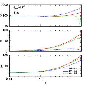
Figure 1: The redshift evolution of $H$, $u$ and $v$. We assume that the geometry of the Universe is flat and fix $\Omega_{m_{0}}=0.27$, then plot the curves for $\omega=-1$, $\omega=-2$ and $\omega=-3$ respectively.

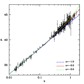
Figure 2: Comparison of the distance moduli between the models with $\omega=-1,-2,-3$ and the SCP SN Ia data set.

We now investigate the constraint on the model. The marginalized PDF of $\omega$ is shown in Fig.3. The best fit value of $\omega$ is about -1.9. Note that $\omega\approx-2$ is required by solar system experiment Klimek , and now we find that the best fit obtained with cosmological data happens to give the same best fit $\omega$ value! This shows that our model predicts dark energy model naturally. The PDF decreases steeply when $\omega>-1.9$ and gently when $\omega<-1.9$, so there is also some probability for $\omega$ to get more negative values.

In Fig.4, we plot the contour map for $\Omega_{m_{0}}$ and $\omega$. We find that the best fit value of $\Omega_{m_{0}}$ is around 0.27 which is consistent with other cosmological observations, e.g. cluster X-ray observations Allen08 . However, more negative values of $\omega$ is also consistent with current observations. The $95.5\%$ C.L.reaches -4.8, when $\Omega_{m_{0}}$ is in the range of $0.24\sim 0.4$.

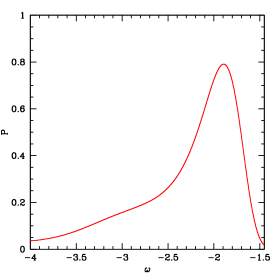
Figure 3: The probability distribution function of $\omega$. We find the best fit value for $\omega$ is about -1.9.

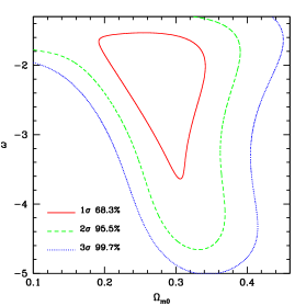
Figure 4: The contour map of $\Omega_{m_{0}}$ and $\omega$. The joint best fit value of $\Omega_{m_{0}}$ and $\omega$ is around (0.27, -1.9). The $1\sigma(68.3\%),2\sigma(95.5\%)$ and $3\sigma(99.7\%)$ C.L. curves are marked by red solid, green dashed and blue dotted lines respectively.

V Summary

By considering a hypersurface-orthogonal spacelike Killing vector field in the 5-dimensional spacetime, the 5D Brans-Dicke theory can be reduced to a 4D theory with the 4-metric coupled to two scalar fields. These two fields could naturally lead to the accelerated expansion of the Universe.

We study the evolution of the two fields and compare the expansion rate with SN Ia observations. The two scalar field would make the Universe evolve as if “matter-dominate” or “dark energy-dominate” when $\omega$ is greater or less than -2. We find that the model is in best agreement with the supernovae data when the 5-dimensional coupling constant $\omega=-1.9\approx-2$, which happens to be also the value required to satisfy the solar system experiments. Furthermore, for this best fit value, the best fit $\Omega_{m_{0}}$ value is about 0.27, in good agreement with other independent measurements such as those derived from X-ray cluster observations. This work is based on the assumption that the 4D gravitational constant $G$ varies extremely slowly so that it can be regarded as a constant at ”low redshift” where the SN Ia data are available. If we further assume $G$ does not change during the whole history of the Universe, then other cosmological observations such as BAO can also be used, we find that in this case the results are almost the same.

In conclusion, the 5-dimensional Brans-Dicke theory could naturally provide two scalar fields which may cause the accelerated expansion, the result is consistent with the SN Ia observation, hence it is a candidate to explain the accelerated expansion of the Universe.

- (1) S. Perlmutter et al., Astrophys. J. 517, 565 (1999)
- (2) A. G. Riess et al., Astron. J. 116, 1009 (1998)
- (3) E. Komatsu et al., (2008) arXiv: 0803.0547
- (4) Y. Gong, T-J. Zhang, T. Lan, X.Chen, arXiv:0810.3572.
- (5) C. Wetterich, Nucl. Phys. B 302, 668 (1988)
- (6) B. Ratra and Peebles, Phys. Rev. D 37, 321 (1988)
- (7) P. G. Ferreira and M. Joyce, Phys. Rev. Lett. 79, 4740 (1997); Phys. Rev. D 58, 023503 (1998).
- (8) R. R. Caldwell, R. Dave, P. J. Steinhardt, Phys. Rev. Lett. 80, 1582 (1998).
- (9) E. J. Copeland, A. R. Liddle, D. Wands, Phys. Rev. D 57, 4686 (1998).
- (10) S. M. Carroll, Phys. Rev. Lett. 81, 3067 (1998).
- (11) I. Zlatev, L. M. Wang, P. J. Steinhardt, Phys. Rev. Lett. 82, 896 (1999).
- (12) P. J. Steinhardt, L. M. Wang, I. Zlatev, Phys. Rev. D 59, 123504 (1999).
- (13) R. R. Caldwell, Phys. Lett. B 545, 23 (2002)
- (14) B. Feng, X. Wang, X. Zhang, Phys. Lett. B 607, 35 (2005).
- (15) T. Chiba, T. Okabe and M. Yamaguchi, Phys. Rev. D 62, 023511 (2000)
- (16) C. Armendariz-Picon, V. Mukhanov and P. J. Steinhardt, Phys. Rev. Lett. 85, 4438 (2000); Phys. Rev. D 63, 103510 (2001).
- (17) T. Padmanabhan, Phys. Rev. D 66, 021301 (2002).
- (18) J. S. Bagla, H. K. Jassal and T. Padmanabhan, Phys. Rev. D 67, 063504 (2003).
- (19) L. R. W. Abramo and F. Finelli, Phys. Lett. B 575, 165 (2003).
- (20) J. M. Aguirregabiria and R. Lazkoz, Phys. Rev. D 69, 123502 (2004).
- (21) Z. K. Guo and Y. Z. Zhang, JCAP. 0408, 010 (2004).
- (22) E. J. Copeland, M. R. Garousi, M. Sami and S. Tsujikawa, Phys. Rev. D 71, 043003 (2005).
- (23) L. Qiang, Y. Ma, M. Han and D. Yu, Phys. Rev. D 71, 061501 (2005).
- (24) S. G. Turyshev et al., Lect. Notes Phys. 648, 301 (2004).
- (25) C. D. Hoyle et al, Phys. Rev. D 70, 042004 (2004).
- (26) M. Blagojevic, Gravitation and Gauge Symmetries, (IOP Publishing, 2002).
- (27) P. G. O. Freund, Nucl. Phys. B209, 146 (1982).
- (28) N. Mohammedi, Phys. Rev. D 65, 104018 (2002).
- (29) F. Darabi, Class. Quantum. Grav. 20, 3385 (2003).
- (30) T. M. Fortier et al., Phys. Rev. Lett. 98, 070801 (2007).
- (31) S. Blatt et al., Phys. Rev. Lett. 100, 140801 (2008).
- (32) E. Peik, B. Lipphardt, H. Schnatz, T. Schneider, C. Tamm and S. G. Karshenboim, Phys. Rev. Lett. 93, 170801 (2004).
- (33) M. Fischer et al., Phys. Rev. Lett. 92, 230802 (2004).
- (34) T. Rosenband et al., Science 319, 1808 (2008).
- (35) M. T. Murphy et al., Lecture Notes Phys. 648, 131 (2004).
- (36) M. T. Murphy, J. K. Webb and V. V. Flambaum, Mon. Not. Roy. Astron. Soc. 384, 1053 (2008).
- (37) M. T. Murphy, J. K. Webb and V. V. Flambaum, Phys. Rev. Lett. 99, 239001 (2007).
- (38) M. Nakashima, R. Nagata and J. Yokoyama, Prog. Theor. Phys. 120, 1207 (2008).
- (39) M. Kowalski et al., (2008) arXiv: 0804.4142.
- (40) A. G. Riess et al., Astrophys. J. 607, 665 (2004).
- (41) A. G. Riess et al., Astrophys. J. 659, 98 (2007).
- (42) P. Astier et al., Astron. Astrophys. 447, 31 (2006).
- (43) G. Miknaitis et al., Astrophys. J. 666, 674 (2007).
- (44) D. J. Eisenstein et al., Astrophys. J. 633, 560 (2005).
- (45) Y. Gong and X. Chen, Phys. Rev. D 76, 123007 (2007).
- (46) M. Klimek, Class. Quant. Grav. 26, 065005 (2009).
- (47) E. J. Copeland, M. Sami and S. Tsujikawa, Int.J.Mod.Phys. D15 (2006) 1753-1936.
- (48) S.W. Allen et al., Mon. Not. R. Astron. Soc. 383, 879 (2008).