Impact of a uniform magnetic field and nonzero temperature on explicit chiral symmetry breaking in QED: Arbitrary hierarchy of energy scales

Abstract

Employing the Schwinger’s proper-time method, we calculate the $\langle\bar{\psi}\psi\rangle$-condensate for massive Dirac fermions of charge $e$ interacting with a uniform magnetic field in a heat bath. We present general results for arbitrary hierarchy of the energy scales involved, namely, the fermion mass $m$, the magnetic field strength $\sqrt{eB}$ and temperature $T$. Moreover, we study particular regimes in detail and reproduce some of the results calculated or anticipated earlier in the literature. We also discuss possible applications of our findings.

1 Introduction

It is well known that the presence of magnetic fields catalyzes the dynamical breakdown of chiral symmetry even for the weakest attractive interaction between fermions. This effect has been dubbed as magnetic catalysis [1, 2, 3, 4]. More recently, the dynamical generation of anomalous magnetic moment of the electron has also been unveiled in [5]. The change in the vacuum structure is governed by the the fermion condensate $\langle\bar{\psi}\psi\rangle$, which serves as an ideal order parameter to capture the details of this effect. At high temperatures, the structure of the phase transition becomes even richer. In Ref. [6], exploring the magnetic catalysis in massless, weakly coupled QED with a magnetic field and temperature, within the context of a constant dynamical mass and only considering the lowest Landau level, it was established that the chiral symmetry is restored above a critical temperature which is much smaller than $\sqrt{eB}$. Under more refined treatment, it was shown in Ref. [7] that symmetry restoration is achieved for a temperature of the order of the dynamically generated mass of the fermion at zero temperature. The phase transition in this case was found to be of second order [8]. Ref. [9] studies the Debye mass and its dependence as a function of magnetic field and temperature by means of computing the vacuum polarization tensor in QED. The work in Ref. [10] deals with the purely thermodynamic part of the one-loop effective potential of a fermion in a constant magnetic field. This article is mainly concerned with the small and large mass expansions for arbitrary values of the magnetic field and temperature, emphasizing the interpretation of this effective potential as a dimensionally reduced one from D to D-2 dimensions. Explicit expressions are not derived for given hierarchies of temperature or magnetic field strengths. This scenario of magnetic fields and finite temperatures is relevant for astrophysical processes such as supernova explosions as well as early universe physics where both the heat bath and the magnetic field participate as key players in this connection. For example, it has been shown by some of us that the inclusion of weak magnetic fields enhances the strength of the first order electroweak phase transition at finite temperature [11]. Fermion condensation by the effects of a magnetic field could give a further boost to these findings. Moreover, the stability of multi-quark droplets using the NJL model at finite temperature and with a homogeneous magnetic field is discussed in Ref. [12], showing that the later promotes the creation of stable droplets and enhances their stability even for quark couplings below the value of the bag constant.

On more terrestrial grounds, relativistic heavy-ion collisions at finite impact parameter offer an opportunity to test the effects of an external magnetic field in the chiral phase transition under extreme conditions [13]. It has recently been shown that in peripheral collisions, a magnetic field of non-negligible strength is generated [14], the origin of which has two components: the effective angular momentum generated by the local imbalance of the momentum carried by the charged colliding nucleons [15], and the addition of currents generated by the spectator nucleons which move in opposite directions in the interaction region. The effect of a strong magnetic field (in RHIC, magnetic fields can reach intensities in the range of $10^{2}-10^{3}MeV^{2}$ for proper times $\tau\lesssim 0.1fm$ [14]) on the chiral phase transition has been predicted to modify a crossover into a weak first-order transition in the linear sigma model [16]. Nevertheless, since the intensity of this field reduces as $1/\tau^{3}$ [14], at $\tau\simeq 1fm$, the field strength has already reduced two orders of magnitude. Therefore, it is desirable to capture the details of the transition over a broad range of values of $eB$. This will become even more important in the LHC, where the magnetic fields in off-center heavy-ion collisions are expected to reach even higher intensities [17].

In this article, we employ the Schwinger’s proper-time method to evaluate the fermion condensate $\langle\bar{\psi}\psi\rangle$ at finite temperature in the presence of an external uniform magnetic field. We present general results without selecting a hierarchy between different energy scales involved, namely, temperature $T$, magnetic field $\sqrt{eB}$ and the bare fermionic mass $m$. We have organized the article as follows. In Sect. II, we calculate $\langle\bar{\psi}\psi\rangle$ at zero temperature in a uniform magnetic field. We also present results for the limiting cases of $\sqrt{eB}\ll m$ and $\sqrt{eB}\gg m$. In Sect. III, the same computation is carried out at finite temperature without magnetic fields. After giving a general expression, we also report analytical expressions in the limit $T\ll m$ as well as $T\gg m$. In Sect. IV, we calculate the fermion condensate in a magnetic field immersed in a heat bath. Starting from the general results, we consider special cases of different hierarchies of energy scales involved ($m$, $B$ and $T$), i.e., $\sqrt{eB}\gg T\gg m$, $T\gg\sqrt{eB}\gg m$ and $T\gg m\gg\sqrt{eB}$. Section V sums up the conclusions.

2 Condensate in vacuum for $B\neq 0$

The $\langle\bar{\psi}\psi\rangle$-condensate is related to the fermion propagator $S(k)$ as follows :

$$\langle\bar{\psi}\psi\rangle=-Tr\int\frac{d^{4}k}{(2\pi)^{4}}S(k)\;.$$ (1)

We are interested in calculating the non-dynamical part of this condensate in the presence of a uniform external magnetic field for a chirally asymmetric theory with fermion bare mass $m$. The part of the condensate associated with the appearance of dynamical masses will be studied elsewhere.

We employ the Schwinger’s proper time method [18] because it is easy to be extended to the case of finite temperature in Sect. IV. Therefore, assuming the magnetic field to be directed along the third spatial direction, we use the expression for the fermion propagator [18] :

$$S_{B}(k) = -i\int^{\infty}_{0}\frac{d\tau}{\cos(eB\tau)}\exp\left[i\tau\left(k^{2}_{||}+\frac{\tan(eB\tau)}{eB\tau}k^{2}_{\perp}-m^{2}+i\epsilon\right)\right]$$

$$\times \left[\exp({ieB\tau\sigma_{3}})(m+\gamma\cdot k_{||}\,)-\frac{\gamma\cdot k_{\perp}}{\cos(eB\tau)}\right]\;.$$

Throughout this work, we use subscript $B$ to denote a quantity in the presence of external magnetic field. Moreover, we employ the notation $(a\cdot b)_{||}\equiv a^{0}b^{0}-a^{3}b^{3}$ and $(a\cdot b)_{\perp}\equiv a^{1}b^{1}+a^{2}b^{2}$ for two arbitrary four-vectors $a^{\mu}$ and $b^{\mu}$. $\sigma_{3}$ is the third Pauli matrix.

Following Ref. [19], the integration over proper time in Eq. (LABEL:schwingerprop) can be cast in the form a sum which runs over the Landau level index $l$, namely

$$S_{B}(k)=i\sum^{\infty}_{l=0}\frac{d_{l}(\frac{k_{\perp}^{2}}{eB})D+d^{\prime}_{l}(\frac{k_{\perp}^{2}}{eB})\bar{D}}{k^{2}_{||}-2leB-m^{2}+i\epsilon}+\frac{{\not\!k_{\perp}}}{k^{2}_{\perp}}\;,$$ (3)

where $d_{l}(\alpha)\equiv(-1)^{n}e^{-\alpha}L^{-1}_{l}(2\alpha)$, $d^{\prime}_{n}=\partial d_{n}/\partial\alpha$  ,

$$D = (m+{\not\!k_{||}})+{\not\!k_{\perp}}\frac{m^{2}-k^{2}_{||}}{{k^{2}_{\perp}}}\;,\qquad\bar{D}=\gamma_{5}{\not\!u}{\not\!b}(m+{\not\!k_{||}})\;,$$ (4)

$L_{l}^{m}(x)$ are the Associated Laguerre polynomials, and $b^{\mu}$ is a four-vector indicating the direction of the magnetic field. Vector $u^{\mu}$ is defined as $(1,\vec{0})$. In case of a heat bath, it describes the plasma rest frame. Using the propagator given in Eq. (3), the chiral condensate can be written as

$$\langle\bar{\psi}\psi\rangle_{B}=\frac{-i4m}{(2\pi)^{4}}\int d^{4}k\sum_{l=0}^{\infty}\frac{(-1)^{l}e^{-\frac{k_{\perp}^{2}}{eB}}L_{l}^{-1}(2\frac{k_{\perp}^{2}}{eB})}{k_{||}^{2}-2leB-m^{2}+i\epsilon}\;.$$ (5)

Starting from this expression, we can establish the equivalence of the result obtained in [2] (a) and [2] (d) (Eqs. (9) and (19), respectively) and [20] (Eq. (9)), obtained through distinct routes and written in an entirely different fashion. In order to do so, we perform the integral over transverse momenta by employing the relation

$$\int_{0}^{\infty}dxe^{-bx}L_{n}(x)=(b-1)^{n}b^{-n-1}\;.$$ (6)

The expression for the condensate then simplifies to

$$\langle\bar{\psi}\psi\rangle_{B}=-\frac{meB}{2\pi^{2}}\sum_{l=0}^{\infty}(2-\delta_{0l})\int_{0}^{\infty}\frac{dk_{3}}{\sqrt{k_{3}^{2}+2leB+m^{2}}}\;.$$ (7)

where we have used the “$i\epsilon$” prescription, that is to say, we decomposed the integral in the principal and imaginary parts. Integrating the above expression term by term, we obtain

$$\langle\bar{\psi}\psi\rangle_{B} = -\frac{2meB}{(2\pi)^{2}}\left\{\ln\left(\frac{1+\sqrt{1+x_{0}^{2}}}{\sqrt{x_{0}^{2}}}\right)+2\sum_{l=1}^{\infty}\ln\left(\frac{1+\sqrt{1+x_{l}^{2}}}{\sqrt{x_{l}^{2}}}\right)\right]\;,$$ (8)

where $x_{l}^{2}=(2leB+m^{2})/\Lambda^{2}$ and $\Lambda$ is the ultraviolet cutoff. This is exactly the result obtained in Ref. [20] by quantizing directly the solutions to the Dirac equation in the external magnetic field.

We can also show that Eq. (7) agrees with the result obtained in Refs. [2] (a) and [2] (d). To see the equivalence, notice that when we derive the integral over $k_{3}$ with respect to $m^{2}$, the remaining integral becomes convergent, acquiring the form

$$\int_{0}^{\infty}\frac{dk_{3}}{{(k_{3}^{2}+\mu^{2})^{\frac{3}{2}}}}=\int_{0}^{\infty}d\eta e^{-\eta\mu^{2}}\;,$$ (9)

with the appropriate choice of $\mu^{2}$. On substituting this expression into Eq. (7) and performing the sum over $l$, (see Ref. [21]) and the integration over $m^{2}$, we are led to the expression for the condensate given in Refs. [2] (a) and [2] (d), i.e.,

$$\langle\bar{\psi}\psi\rangle_{B}=-\frac{meB}{(2\pi)^{2}}\int_{\frac{1}{\Lambda^{2}}}^{\infty}\frac{d\eta}{\eta}e^{-\eta m^{2}}\coth(\eta eB)\;,$$ (10)

where $\Lambda$ is the ultraviolet cut-off of Eq. (8). We have thus established the equivalence of Eq. (8) and Eq. (10), In order to calculate purely the magnetic field effect, we need to subtract out the vacuum piece. Working with Eq. (10), we obtain

$$\langle\bar{\psi}\psi\rangle_{0} = -\frac{m}{(2\pi)^{2}}\int_{\frac{1}{\Lambda^{2}}}^{\infty}\frac{d\eta}{\eta^{2}}e^{-\eta m^{2}}.$$ (11)

This result is the origin of the quadratic divergence in the condensate in the vacuum piece. Subtracting out the vacuum part from Eq. (10), the magnetic field dependent fermion condensate is

$$\Delta\left<\overline{\psi}\psi\right>_{B} \equiv \left<\overline{\psi}\psi\right>_{B}-\left<\overline{\psi}\psi\right>_{0}$$ (12)

$$=\frac{-m}{(2\pi)^{2}}\int_{0}^{\infty}\frac{d\eta}{\eta^{2}}e^{-\eta m^{2}}\left[eB\eta\coth(eB\eta)-1\right],$$

which is finite.

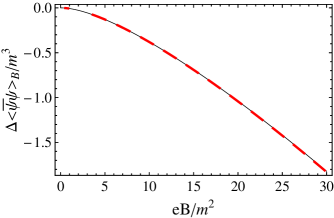
Figure 1: Magnetic field dependent fermion condensate in units of $m^{3}$ as a function of $eB/m^{2}$. Solid line: exact result, Eq. (12). Thick dashed line: exact result deduced from Eq. (12) of Ref. [2] (a), i.e., Eq. (13).

Note that the above expression has been obtained for an arbitrary value of the field strength $eB$, as compared to $m$. The numerical plot of the condensate as a function of field strength is shown in Fig. 1 as a solid line. In magnitude, it increases with the magnetic field strength. The same condensate can be easily extracted from Eq. (15) of the Ref. [2] (a). The equivalence can be established by taking into account the fact that the condensate is given by the derivative of the effective potential, $dV(\rho)/d\rho$, where $\rho$ is a convenient combination of the fields involved. The magnetic field dependent condensate would be given by

$$\Delta\left<\overline{\psi}\psi\right>_{B}=\frac{dV(\rho)}{d\rho}-\left[\frac{dV(\rho)}{d\rho}\right]_{B=0}\;.$$ (13)

This expression has been plotted in Fig. 1 as a thick dashed line. This lies exactly on top of the curve representing Eq. (12), establishing the correctness of our result.

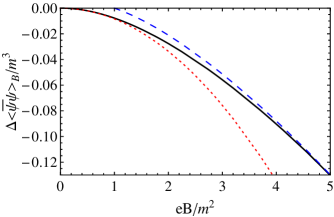
Figure 2: Magnetic field dependent fermion condensate in units of $m^{3}$ as a function of $eB/m^{2}$. Solid line: exact result, Eq. (12). Dashed line: strong field limit, Eq. (14). Dotted line: weak field limit, Eq. (15).

From the general expression, we can deduce the behavior of the condensate for the values of the magnetic field under consideration. For example, it is well known that in the strong field limit, the main contribution comes from the lowest Landau level (LLL) in Eq. (8). In terms of the integral Eq. (12), the same contribution comes from the interval $[1,\infty)$ [21]. Calculating either way, the analytic expression for the result is

$$\Delta\langle\overline{\psi}\psi\rangle_{B}\stackrel{{\scriptstyle\sqrt{eB}\gg m}}{{\longrightarrow}}-\frac{meB}{(2\pi)^{2}}\left[\ln\left(\frac{eB}{m^{2}}\right)\!-\!\gamma_{E}\!-1\!\right].$$ (14)

This contribution has been displayed by the dashed line in Fig. 2. As expected, it matches on to the exact result in the intense field limit.

We also obtain a closed expression in the weak field limit :

$$\Delta\langle\overline{\psi}\psi\rangle_{B}\stackrel{{\scriptstyle\sqrt{eB}\ll m}}{{\longrightarrow}}-\frac{(eB)^{2}}{(2\pi)^{2}m}\;,$$ (15)

represented by the dotted line in Fig. 2. It nicely reproduces the exact curve for $eB\ll m^{2}$. Eqs. (12), (14), and (15) are the main results of this section. We now turn our attention to the case of the condensate at finite temperature in absence of external magnetic fields.

3 Condensate at finite temperature and $B=0$

In this section, we shall study the effect of the heat bath (or thermal fluctuations) at temperature $T$ on the fermion condensate in the absence of any external field. On comparison with the previous section, we find that the effect of the finite temperature is opposite to that of the magnetic field. In order to incorporate the effects of a thermal bath, we use the imaginary-time formulation of thermal field theory (see, for example, [22]). In this formalism, we replace integration over the time component $k_{0}$ with a sum over discrete (Matsubara) frequencies according to the prescription

$$\int\frac{d^{4}k}{(2\pi)^{4}}f(k)\rightarrow T\sum_{n}\int\frac{d^{3}k}{(2\pi)^{3}}f(\omega_{n},{\bf k})$$ (16)

where $\omega_{n}=(2n+1)\pi T$ for fermions, with $n=0,\pm 1,\pm 2,\pm 3\ldots$, and $T$ is the temperature. We shall use the convenient notation

$$T\sum_{n}\int\frac{d^{3}k}{(2\pi)^{3}}f(\omega_{n},{\bf k})\equiv\int_{\beta}f(\omega_{n},{\bf k})\;,$$ (17)

to denote integration and summation over Matsubara frequencies $\omega_{n}$, with $\beta=1/T$. At finite temperature, the fermion condensate is

$$\langle\bar{\psi}\psi\rangle^{T} = -4m\int_{\beta}\frac{1}{\omega_{n}^{2}+\omega_{k}^{2}}=-\frac{m\beta^{2}}{\pi^{2}}\int_{\beta}\int_{0}^{\infty}ds\ e^{-s\left(\frac{\omega_{k}}{2\pi T}\right)^{2}}e^{-s\left(n+\frac{1}{2}\right)^{2}}.$$ (18)

The superscript $T$, from now on, denotes a quantity affected by the heat bath. Moreover, $\omega_{k}^{2}=k^{2}+m^{2}$. Note that we have made use of the identity $a^{-1}=\int_{0}^{\infty}ds\ e^{-sa}$, which is valid for $Re[a]>0$. As a result, the integral over momenta is Gaussian and that the sum over Matsubara frequencies gets decoupled from this integral.

Since the sum over Matsubara frequencies converges slowly, we perform the sum by means of the Poisson resummation formula,

$$\sum_{n}e^{-s\left(n+\frac{1}{2}\right)^{2}} = \left(\frac{\pi}{s}\right)^{\frac{1}{2}}\sum_{n}(-1)^{n}e^{-\frac{n^{2}\pi^{2}}{s}}.$$ (19)

It is well known that once the sum over Matsubara frequencies is carried out, the result contains the vacuum contribution. Particularly, in the above expression, the vacuum contribution comes from the term $n=0$. To see this explicitly, we only need to replace Eq. (19) with $n=0$ into Eq. (18). Thus

$$\langle\bar{\psi}\psi\rangle^{0} = -\frac{m\beta^{2}}{\pi^{3/2}}\int\frac{d^{3}k}{(2\pi)^{3}}\int_{0}^{\infty}\frac{ds}{s^{\frac{1}{2}}}e^{-s\left(\frac{\omega_{k}}{2\pi T}\right)^{2}}.$$ (20)

The integration over $s$ is straightforward, yielding

$$\langle\bar{\psi}\psi\rangle^{0} = -2m\int\frac{d^{3}k}{(2\pi)^{3}}\frac{1}{\sqrt{k^{2}+m^{2}}},$$ (21)

which corresponds precisely to the fermion condensate in vacuum.

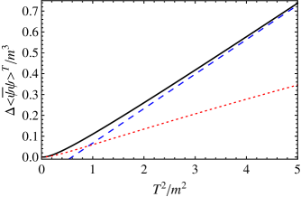
Figure 3: Temperature dependent fermion condensate in the units of $m^{3}$ as a function of $T^{2}/m^{2}$. Solid line: exact result, Eq. (25). Dashed line: high temperature limit, Eq. (27). Dotted line: low temperature limit, Eq. (28).

Now we proceed to analyze the sum of the remaining terms with $n\neq 0$. These terms contain purely thermal contributions. In order to do so, the first step is to perform the integral over momentum in Eq. (18),

$$\int\frac{d^{3}k}{(2\pi)^{3}}e^{-s\frac{k^{2}}{(2\pi T)^{2}}}=\left(\sqrt{\frac{\pi}{s}}\,T\right)^{3}\;.$$ (22)

Inserting the above result along with Eq. (19) into Eq. (18), we find that

$$\Delta\langle\bar{\psi}\psi\rangle^{T} = \langle\bar{\psi}\psi\rangle^{T}-\langle\bar{\psi}\psi\rangle^{0}$$ (23)

$$=mT^{2}\sum_{n\neq 0}(-1)^{n+1}\int_{0}^{\infty}\frac{ds}{s^{2}}e^{-\left[\left(\frac{m}{2\pi T}\right)^{2}s+\frac{\pi^{2}n^{2}}{s}\right]}\;.$$

This result can be further simplified with the help of the identity [23],

$$\int_{0}^{\infty}ds\ s^{-\nu-1}e^{-\gamma s-\frac{\delta}{s}}=2\left(\frac{\gamma}{\delta}\right)^{\frac{\nu}{2}}K_{\nu}(2\sqrt{\delta\gamma})\,,$$ (24)

valid for $\mbox{Re}[\delta]>0$ and $\mbox{Re}[\gamma]>0$, and where $K_{\nu}(x)$ are the Bessel functions of the second kind. We thus find the temperature dependent fermion condensate to be

$$\Delta\langle\bar{\psi}\psi\rangle^{T} = -\frac{8mT^{2}}{(2\pi)^{2}}\sum_{n=1}^{\infty}\frac{(-1)^{n}}{n}\frac{m}{T}K_{1}\left(n\frac{m}{T}\right)\;.$$ (25)

This is an exact result, valid for all ranges of temperature and mass. Numerically, it converges rapidly for increasing values of Matsubara frequencies. It is plotted as a solid line in Fig. 3. The condensate is positive and it rises with increasing temperature. Notice that the relative sign between the thermal and magnetic condensates (recall Fig. 2), indicates that the heat bath acts opposite to the effect of the magnetic field.

From the exact result, we can extract the behavior of the condensate under extreme conditions of high temperature in a closed form. To this end, we make use of the identity [24]

$$\sum_{n=1}^{\infty}\frac{1}{n}K_{1}(nz)\cos(n\phi) = -\frac{z}{4}\left[\ln\left(\frac{z}{4\pi}\right)+\gamma_{E}-\frac{1}{2}\right]+\frac{1}{z}\left[\frac{1}{4}\phi^{2}-\frac{\pi}{2}\phi+\frac{\pi^{2}}{6}\right]$$ (26)

$$-\frac{\pi}{2z}\sum_{l\neq 0}\left[\sqrt{z^{2}+(\phi-2\pi l)^{2}}-|\phi-2\pi l|-\frac{z^{2}}{4\pi|l|}\right].$$

Notice that when $\phi=\pi$ the sum on the l.h.s reduces to the sum in Eq. (25). In the high temperature limit, i.e., $m/T\ll 1$ (or $z\ll 1$) the first and third terms on the r.h.s of the identity vanish. This allows us to evaluate the fermion condensate analytically in this limit :

$$\Delta\langle\bar{\psi}\psi\rangle^{T} \stackrel{{\scriptstyle T\gg m}}{{\longrightarrow}} \frac{mT^{2}}{6}\;.$$ (27)

It is displayed in Fig. 3 with a dashed line. The exact result aligns itself with Eq. (27) in the high temperature limit. The low temperature behavior for the temperature dependent condensate can be obtained from Eq. (25) by means of an asymptotic expansion for the Bessel functions near infinity. We can then perform the sum over $n$ term by term. We again obtain a closed expression in this regime,

$$\Delta\left<\overline{\psi}\psi\right>_{T} \stackrel{{\scriptstyle T\ll m}}{{\longrightarrow}} \frac{1}{2}\left(\frac{2mT}{\pi}\right)^{\frac{3}{2}}e^{-\frac{m}{T}}\;.$$ (28)

This result is depicted in Fig. 3 by the dotted line. Note that the high temperature limit, Eq. (27), breaks down at lower values of temperature and is taken over by Eq. (28) to mimic the exact result. Eqs. (25), (27), and (28) constitute the main results of this section. The combined effect of an external uniform magnetic field and a heat bath on the fermion condensate is studied in the next section.

4 Condensate in a heat bath with $B\neq 0$

In previous sections, we have observed that the effects of the external uniform magnetic field and the thermal bath on the fermion condensate are diametrically opposed. A natural and more relevant scenario is to study the combined effect of these two antagonic agents on $\langle\bar{\psi}\psi\rangle$. We apply the procedure similar to the one developed in the previous two sections and arrive at the following expression :

$$\Delta\langle\bar{\psi}\psi\rangle_{B}^{T} = -\frac{meB}{\pi^{2}}\sum_{l=0}^{\infty}(2-\delta_{0l})\sum_{n=1}^{\infty}(-1)^{n}K_{0}\left(n\frac{\sqrt{2leB+m^{2}}}{T}\right)$$ (29)

$$+ \Delta\left<\overline{\psi}\psi\right>_{B}\;.$$

Notice that the first term takes into account the effects of thermal bath and the external magnetic field on the fermion condensate, while the second corresponds to the condensate in vacuum with a background magnetic field. This is one of the main results of our paper.

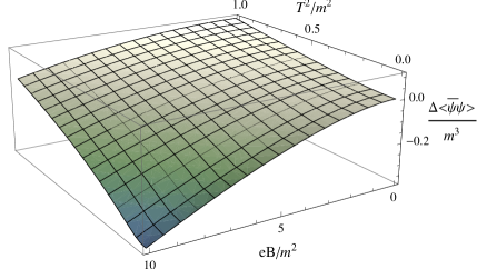
Figure 4: Temperature and magnetic field dependent fermion condensate as a function of $eB/m^{2}$ and $T^{2}/m^{2}$.

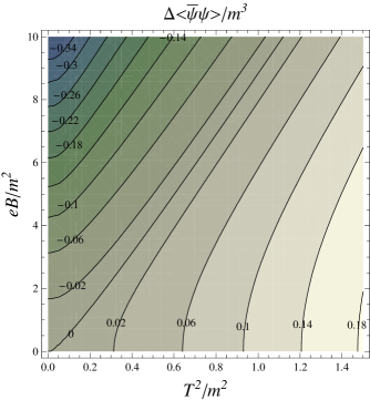
Figure 5: Contour plot for the temperature and magnetic field dependent fermion condensate as a function of $eB/m^{2}$ and $T^{2}/m^{2}$.

Eq. (29) can also be cast in the following form :

$$\Delta\left<\overline{\psi}\psi\right>_{B}^{T} = \frac{2meB}{(2\pi)^{2}}\sum_{n=1}^{\infty}(-1)^{n+1}\int_{0}^{\infty}\frac{ds}{s}e^{-\left[\frac{m^{2}}{(2\pi T)^{2}}s+\frac{\pi^{2}n^{2}}{s}\right]}\coth\left(\frac{eBs}{(2\pi T)^{2}}\right)$$ (30)

$$+ \Delta\left<\overline{\psi}\psi\right>_{B}\;.$$

This exact expression can also be written in terms of the Jacobi $\Theta_{4}$ function originating from the sum over $n$, [25] as follows :

$$\Delta\left<\overline{\psi}\psi\right>_{B}^{T} = -\frac{meB}{(2\pi)^{2}}\int_{0}^{\infty}\frac{ds}{s}\left[\Theta_{4}(0;e^{-\frac{\pi^{2}}{s}})-1\right]e^{-\frac{m^{2}}{(2\pi T)^{2}}s}\coth\left(\frac{eBs}{(2\pi T)^{2}}\right)$$ (31)

$$+ \Delta\left<\overline{\psi}\psi\right>_{B}\;.$$

The exact form is plotted in Fig. 4. Note that at high temperatures and weak magnetic field (the farthest edge of the cube), the condensate is positive. For low temperatures and intense magnetic fields (the closest edge of the cube), playing the dominant and opposite role, the magnetic field pulls down the condensate to its large negative values. In the region where the condensate does not deviate much from its zero value (from the right edge of the cube towards the left edge), temperature and magnetic fields manage to nullify the effect of each other. This effect is most visible in the contour plot displayed in Fig. 5.

Starting from Eq. (30), we can analyze different scenarios of relative strengths of the mass $m$, the magnetic field $eB$ and the temperature $T$. In the following sub-sections, we discuss various hierarchies of interest, of the energy scales involved : intense magnetic fields, i.e., $m\ll T\ll\sqrt{eB}$, intermediate magnetic fields, namely $m\ll\sqrt{eB}\ll T$, and weak magnetic fields, $\sqrt{eB}\ll m\ll T$.

4.1 Strong Field

Let us begin by considering the following hierarchy among the energy scales involved: $m\ll T\ll\sqrt{eB}$. In such a scenario, the main contribution comes from the LLL, i.e., $l=0$ in Eq. (29). In this regime, the condensate is given by

$$\Delta\langle\bar{\psi}\psi\rangle_{B}^{T} = -\frac{meB}{\pi^{2}}\sum_{n=1}^{\infty}(-1)^{n}K_{0}\left(n\frac{m}{T}\right)-\frac{meB}{(2\pi)^{2}}\left[\ln\left(\frac{eB}{m^{2}}\right)-\gamma_{E}-1\right]\;.$$ (32)

Furthermore, we again use Eq. (26) to perform the high temperature expansion ($m\ll T$) :

$$2\sum_{n=1}^{\infty}(-1)^{n}K_{0}\left(n\frac{m}{T}\right) \stackrel{{\scriptstyle m\ll T}}{{\rightarrow}} \gamma_{E}-1+\ln\left(\frac{m}{\pi T}\right)\;.$$ (33)

Substituting this expression into Eq. (32) and using Eq. (15) yields the fermion condensate

$$\Delta\left<\overline{\psi}\psi\right>_{B}^{T}=-\frac{meB}{(2\pi)^{2}}\left[\ln\left(\frac{eB}{\pi^{2}T^{2}}\right)+\gamma_{E}-3\right]\;.$$ (34)

This is drawn as the dashed line in Fig. 6 against the exact result for a given value of temperature, represented by the solid line. Note that it fits the exact result very well when the magnetic field intensity is sufficiently large as compared to other energy scales in the problem. However, this LLL approximation breaks down when magnetic fields are lowered, and we have to resort to other approximation schemes as detailed in the sub-sections to follow.

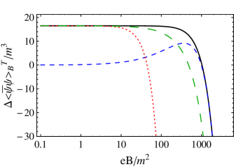
Figure 6: Temperature and magnetic field dependent fermion condensate as a function of $eB/m^{2}$ at fixed $T$. Solid line: exact (numerical) result, Eq. (30). Dashed line: strong field limit, Eq. (34). Long Dashed line: intermediate field limit (numerical), Eq. (36). Dotted line: weak field limit, Eq. (41).

4.2 Field of Intermediate Intensity

In this regime, the temperature dominates over any other energy scale. Therefore, we expect that the main contribution to fermion condensate comes from the thermal bath. In order to confirm this, we take the high temperature limit of Eq. (29). Employing Eq. (33), we arrive at

$$\Delta\left<\overline{\psi}\psi\right>_{B}^{T} = -\frac{2meB}{(2\pi)^{2}}\sum_{l=0}^{\infty}(2-\delta_{l0})\left[\ln\left(\frac{\sqrt{2leB+m^{2}}}{4\pi T}\right)+\gamma_{E}-1\right]$$ (35)

$$- \frac{meB}{(2\pi)^{2}}\left[\ln\left(\frac{eB}{m^{2}}\right)-\gamma_{E}-1\right]\;,$$

where we have also made use of the fact that $\sqrt{eB}\gg m$, Eq. (14) As the magnetic field provides an intermediate energy scale, fermions can access all the Landau levels and we have to perform the sum over all of them. This is achieved by invoking the procedure outlined in Ref. [21] :

$$\Delta\left<\overline{\psi}\psi\right>_{B}^{T} = \frac{meB}{(2\pi)^{2}}\int_{\frac{3}{2\pi^{2}T^{2}}}^{\infty}\frac{d\eta}{\eta}e^{-\eta m^{2}}\coth(\eta eB)$$ (36)

$$- \frac{meB}{(2\pi)^{2}}\left[\ln\left(\frac{eB}{m^{2}}\right)-\gamma_{E}-1\right]\;.$$

Notice that we have introduced an infrared cutoff $(2/3)\pi^{2}T^{2}$. This is due to the fact that in the limit $eB\rightarrow 0$, each component of the transverse momentum contributes to the thermal bath with a factor of $(1/3)\pi^{2}T^{2}$. In this kinematical region, we cannot perform any other approximation and hence a closed expression alludes us. In Fig. 6, we plot the numerical results for Eq. (36) in the form of the long dashed line. It nicely captures the correct intermediate field range.

4.3 Weak field

We finally consider the weak field scenario $\sqrt{eB}\ll m\ll T$. In this case, we have to perform sum over all Landau levels, since the gap between energy levels is small and thermal fluctuations can bring fermions from one level to a higher one easily. Notice that Eq. (26) no longer provides a useful starting point because the sum over Landau levels exhibits a divergence. Nevertheless, we can perform a weak field expansion in the fermion propagator, Eq. (3), which allows to perform the summation over Landau levels. The resulting fermion propagator is then written as a power series in $eB$. Up to order $(eB)^{2}$ it reads [26]

$$S_{B}(k) \approx \frac{{\not\!k}+m}{k^{2}-m^{2}}+\frac{\gamma_{5}{\not\!u}{\not\!b}({\not\!k}_{||}+m)eB}{(k^{2}-m^{2})^{2}}$$ (37)

$$- \frac{2(eB)^{2}k_{\perp}^{2}}{(k^{2}-m^{2})^{4}}\left(m+{\not\!k}_{||}+{\not\!k}_{\perp}\frac{m^{2}-k^{2}}{k_{\perp}^{2}}\right).$$

Substituting this expansion into Eq. (1), the fermion condensate in the weak field limit is given by

$$\langle\bar{\psi}\psi\rangle_{B} = -iTr\int\frac{d^{4}k}{(2\pi)^{4}}\left[\frac{{\not\!k}+m}{k^{2}-m^{2}}+\frac{\gamma_{5}{\not\!u}{\not\!b}({\not\!k}_{||}+m)eB}{(k^{2}-m^{2})^{2}}\right.$$ (38)

$$-\frac{2(eB)^{2}k_{\perp}^{2}}{(k^{2}-m^{2})^{4}}\left.\left(m+{\not\!k}_{||}+{\not\!k}_{\perp}\frac{m^{2}-k^{2}}{k_{\perp}^{2}}\right)\right]\;.$$

Notice that the term linear in the magnetic field vanishes when we take the trace. Thus,

$$\langle\bar{\psi}\psi\rangle_{B} = -i4m\int\frac{d^{4}k}{(2\pi)^{4}}\left[\frac{1}{k^{2}-m^{2}}-\frac{2(eB)^{2}k_{\perp}^{2}}{(k^{2}-m^{2})^{4}}\right].$$ (39)

With the prescriptions of the imaginary time formalism, Eq. (16), the fermion condensate in the weak field limit at finite temperature can be written as

$$\langle\bar{\psi}\psi\rangle^{T}_{B} = -4mT\sum_{n}\int\frac{d^{3}k}{(2\pi)^{3}}\left[\frac{1}{\omega_{n}^{2}+k^{2}+m^{2}}+\frac{2(eB)^{2}k_{\perp}^{2}}{(\omega_{n}^{2}+k^{2}+m^{2})^{4}}\right]\;.$$ (40)

Notice that the first term was calculated in Eq. (18) with the result shown in Eq. (27). Given the hierarchy of energy scales in this limit, the thermal component that comes from the second term is negligible. Therefore, the main contribution comes from the vacuum part. After some routine algebra, the condensate in this limit is given by the following closed expression :

$$\Delta\left<\overline{\psi}\psi\right>^{T}_{B} = \frac{mT^{2}}{6}\left[1-\frac{7\zeta(3)}{8\pi^{4}}\frac{(eB)^{2}}{T^{4}}-\frac{1}{(2\pi^{2})}\frac{(eB)^{2}}{m^{2}T^{2}}\right]\;,$$ (41)

where $\zeta(x)$ is the Riemann zeta function. This expression is depicted by the dotted line in Fig. 6, which lies on top of the exact result in the limit of weak magnetic fields. With increasing values of the magnetic field, this result starts becoming more and more inaccurate while the intermediate field limit, Eq. (36), still preserves its validity. For intense magnetic fields, Eq. (34) takes over as the adequate description of reality.

5 Conclusions

The simultaneous presence of finite temperature and external magnetic fields is a realistic situation in the physics of the early universe [11], astronomical objects and even heavy ion collisions [13]. Therefore, it is important to estimate the effect of these conditions on the fermion mass and the fermion-anti-fermion condensate. Moreover, in all the practical situations in cosmology, astrophysics, or heavy ion collisions, charged fermions have a bare mass as long as the electroweak phase transition has taken place. Its contribution to the mass gap or the $\langle\bar{\psi}\psi\rangle$ condensate is an important question whose relevance has been highlighted in several recent works, both in the vacuum, [27], as well as in the presence of an external magnetic field, [28].

In this article, we present a detailed study of this effect in QED on the $\langle\bar{\psi}\psi\rangle$ condensate for the bare fermionic mass $m$ in the absence of self interactions. Most importantly, our results are valid for an arbitrary hierarchy of the energy scales involved, namely, the fermion mass $m$, the external magnetic field strength $\sqrt{eB},$ and the temperature $T$. This is achieved by carrying out the sum over all the Landau levels and all the Matsubara frequencies. To the best of our knowledge, no such complete calculation exists so far in the literature. The effect of the temperature and the magnetic fields are diametrically opposed, thus tending to nullify each other. We also take several physically relevant limits of our general results and arrive at closed expressions for particular regimes of $T$, $\sqrt{eB}$ and $m$. This analysis explicitly reveals the domain of validity of each and every approximation employed : $\sqrt{eB}\gg T\gg m$, $T\gg\sqrt{eB}\gg m$ and $T\gg m\gg\sqrt{eB}$. We also present exact results for the cases when either temperature or the magnetic field is absent. For special cases, we reproduce the results already known in the literature. The main results of our article are : Eqs. (12), (14), and (15) for $T=0,~{}B\neq 0$, Eqs. (25), (27), and( 28) for $T\neq 0,~{}B=0$ and Eqs. (30), (34), (36), and (41) for $T\neq 0,~{}B\neq 0$. A natural next step is to include the dynamical interaction effects while still preserving the arbitrariness of temperature as well as external magnetic field. All this is for future.

References

References

- [1] (a) K G Klimenko 1992 Z. Phys. C54 323; (b) K G Klimenko 1992 Theor. Math. Phys. 89 1161 [english translation of the russian paper K G Klimenko 1991 Teor. Mat. Fiz. 89 211]; (c) K G Klimenko 1992 Theor. Math. Phys. 90 1 [english translation of the russian paper K G Klimenko 1992 Teor. Mat. Fiz. 90 3].
- [2] (a) V P Gusynin, V A Miransky and I A Shovkovy 1995 Phys. Lett. B 349 477; (b) V P Gusynin, V A Miransky and I A Shovkovy 1995 Phys. Rev. D 52 4718; (c) V P Gusynin, V A Miransky and I A Shovkovy 1995 Phys. Rev. D 52 4747; (d) V P Gusynin, V A Miransky and I A Shovkovy 1996 Nucl. Phys. B 462 249; (e) V P Gusynin, V A Miransky and I A Shovkovy 1999 Nucl. Phys. B 563 361; (f) V P Gusynin, V A Miransky and I A Shovkovy 1994 Phys. Rev. Lett. 73 3499.
- [3] (a) D-S Lee, C N Leung and Y J Ng 1997 Phys. Rev. D 55 6504; (b) D K Hong 1998 Phys. Rev. D 57 3759; (c) E J Ferrer and V de la Incera 2000 Phys. Lett. B 481 287.
- [4] (a) A Ayala, A Bashir, A Raya and E. Rojas 2006 Phys. Rev. D 73 105009; (b) A Ayala, A Bashir, A Raya and E. Rojas 2008 Phys. Rev. D 77 093004; (c) N Sadooghi and K Sohrabi Anaraki 2008 Phys. Rev. D 78 125019.
- [5] E J Ferrer and V de la Incera 2009 Phys. Rev. Lett. 102 050402; E J Ferrer and V de la Incera 2009 Nucl. Phys. B 824 217.
- [6] D S Lee, C N Leung and Y J Ng 1997 Phys. Rev. D 55 6504.
- [7] V P Gusynin and I A Shovkovy 1997 Phys. Rev. D 56 5251.
- [8] D S Lee, C N Leung and Y J Ng 1998 Phys. Rev. D 57 5224.
- [9] J Alexandre 2001 Phys. Rev. D 63 073010.
- [10] H-T Sato 1998 J. Math. Phys. 39 4540.
- [11] A Sánchez, A Ayala and G Piccinelli 2007 Phys. Rev. D 75 043004.
- [12] D Ebert and K G Klimenko 2003 Nucl. Phys. A 728 203; K G Klimenko and D Ebert, 2005 Phys. At. Nucl. 68 124.
- [13] For a recent and comprehensive review, see the proceedings of the workshop on high pt physics at LHC PoS(LHC07).
- [14] D E Kharzeev, L D McLerran and H J Warringa 2008 Nucl. Phys. A 803 227.
- [15] (a) Z-T Liang and X-N Wang 2005 Phys. Rev. Lett. 94 102301; (b) F Becattini, F Piccinini and J Rizzo 2008 Phys. Rev. C 77 024906.
- [16] E S Fraga and A J Mizher 2008 Phys. Rev. D 78 025016.
- [17] V Skokov, A Illarionov and V Toneev Estimate of the magnetic field strength in heavy-ion collisions e-pront: arXiv:0907.1396 [nucl-th].
- [18] J Schwinger 1951 Phys. Rev. 82 664.
- [19] A Chodos, K Everding, D A Owen 1990 Phys. Rev. D 42, 2881.
- [20] M de J Anguiano-Galicia, A Bashir and A Raya 2007 Phys. Rev. D 76 127702.
- [21] V B Berestetskii, E M Lifshitz and L P Pitaevskii 1982 Quantum Electrodynamics (Pergamon Press).
- [22] J I Kapusta 1989 Finite Temperature Field Theory (1st. edition, Cambridge University Press).
- [23] I S Gradshteyn and I M Ryzhik 2000 Table of Integrals, Series and Products (Academic Press) p. 567.
- [24] P N Meisinger and M C Ogilvie 2002 Phys. Rev. D 65 056013.
- [25] E J Ferrer, V P Gusynin and V de la Incera 2003 Eur. Phys. J. B 33, 397.
- [26] T-K Chyi, C-W Hwang, W F Kao, G-L Lin, K-W Ng and J-J. Tseng 2000 Phys. Rev. D 62, 105014.
- [27] L Chang, Y-X Liu, M S Bhagwat, C D Roberts and S V Wright 2007 Phys. Rev. C 75, 015201.
- [28] S-Y Wang 2008 Phys. Rev. D 77, 025031; K G Klimenko and V Ch Zhukovsky 2008 Phys. Lett. B 665 352; E Rojas Radiative and non-perturbative corrections to the electron mass and the anomalous magnetic moment in the presence of an external magnetic field of arbitrary strength. e-Print: arXiv:0811.1066 [hep-ph].