New Physically Realistic Solutions for Charged Fluid Spheres

Abstract

A new class of solutions to the coupled, spherically symmetric Einstein-Maxwell equations for a compact material source is constructed. Some of these solutions can be made to satisfy a number of requirements for being physically relevant, including having a causal speed of sound. In the case of vanishing charge these solutions reduce to those found by Bayin and Tolman. Only the latter can be considered as having physically realistic properties.

1 Introduction

One of the most fundamental problems in general relativity is the construction of exact solutions to the Einstein equations (or the Einstein equations coupled to other equations associated with fundamental physical theories). An even more challenging problem is is to find solutions that might represent physically realizable systems that could possibly occur in nature. It is well known that of the many solutions to the systems of equations derived from the Einstein equations lead to unphysical behaviour. In many cases, the spacetimes constructed may be truly singular even in the presence of matter or other fields. Alternatively negative energy densities and/or negative pressures are often required in order to meet regularity conditions or boundary conditions that are imposed upon the metric or other geometric objects. In other cases where energy densities and pressures are positive, often one finds that the speed of sound violates causality by being greater than the speed of light. For example constant density configurations, where the pressure has a radial dependence to ensure that the interior solution remains static will lead to infinite sound speeds. Charged dust solutions on the other hand have zero sound speed. They require such a fine balance between the mass and charge distributions that they are almost always unstable to any perturbations. They either undergo gravitational collapse or fly apart due to electrostatic repulsion.

This paper will present a new solution to the spherically symmetric time independent Einstein-Maxwell system of equations that govern the behaviour of the space-time in the interior of a charged fluid sphere. At the outer boundary the solutions will be matched to the external vacuum solution for the field equations i.e. the Reissner-Nordström solution. It will be demonstrated that some of these solutions have parameter values that lead to physically realistic properties.

While the total number of known exact interior solutions to the Einstein-Maxwell equations is much smaller than their uncharged counterparts, the number of solutions that can be said to be physically relevant is small. A review of such solutions has been provided by Ivanov [1] and this makes a good starting place for understanding the different approaches that have been taken and the results obtained from those approaches. In some instances corrections to some of the original papers are provided. The most commonly used methods employ either isotropic coordinates (where the problem was first discussed by Papapetrou [2] and Majumdar [3]) or curvature (i.e. Schwarzschild-like) coordinates.

As mentioned in the introductory paragraph above, this paper will be primarily concerned with the construction of physically “interesting” solutions that might arise from regular initial conditions for charge and mass densities along with realistic pressure distributions. The motivations for this are to find compact charged fluid configurations that might represent realistic sources for the exterior vacuum Reissner-Nordström solutions. In particular one can ask whether it is possible to find realistic solutions for the extreme case where the total charge is equal to the total mass. A second motivation is to determine the possible end states for systems that have collapsed gravitationally but due to the repulsive nature of the electrostatic interaction are unable to form black holes and result in stable configurations.

The approach to be taken here is to write the Einstein-Maxwell system in curvature coordinates. The Einstein equations will yield three equations for two metric functions in terms of the mass density, the charge aspect and the fluid pressure. The Maxwell equations simply state the the electrostatic Maxwell field is just the Coulomb field in a spherically symmetric space time. The solution will be given in terms of explicit closed-form functions of the radial coordinate for the two metric coefficients, a mass density, a charge aspect (the integrated charge density) and the pressure of the fluid.

The review by Ivanov outlines that various ansätse that have been utilized to find exact solutions. Essentially one gives two out of the five functions and uses the Einstein-Maxwell equations to construct the remainder. Of course some methods of solution are easier than others, particularly if one is not concerned with ensuring that the solution have a physical interpretation. The simplest method is to give the functional dependence of the metric functions and construct the remaining variables from the derivatives on the “left-hand-side” of the differential equations. On the other hand giving the mass and/or charge distributions along with an equation of state of the form $P=P(\rho)$ requires solving a set of nonlinear coupled differential equations. But the method has the advantage that there is some control over the physics. Other methods use a combination of the two approaches.

The requirements that make a solution physically relevant has had much discussion in the literature. (See e.g.  the reviews by Delgaty and Lake [4] and Finch and Skea [5] that analyze over one hundred known solutions for uncharged, spherically symmetric, fluid solutions in general relativity.) Those that we expect to meet are the following:

1. The metric coefficients are regular everywhere including at the origin $r=0$.

2. The metric functions match to the Reissner-Nordström functions at the fluid-vacuum interface.

3. The mass density is positive and decreasing outward toward the boundary.

4. The integrated charge and mass increase outward to give the RN parameters at the boundary.

5. The pressure $P$ is positive and finite everywhere inside the fluid

6. The pressure vanishes at the fluid boundary with the vacuum.

7. The speed of sound $v_{\rm s}=(dP/d\rho)^{1/2}$ is causal ($0\leq v\leq 1$).

8. The speed of sound $v_{\rm s}=(dP/d\rho)^{1/2}$ monotonically decreases with increasing $r$.

9. Both the pressure and mass density are decreasing functions of $r$: $dP/dr<0$ and $d\rho/dr<0$.

This list is not necessarily exhaustive but does include all of the requirements presented by Delgaty and Lake in their extensive review of exact fluid sphere solutions. Supplementary conditions that define what Finch and Skea call “interesting solutions” have been reviewed in that manuscript. These extra conditions include: an explicit equation of state in the form $P=P(\rho)$, and non-numerical solutions to the differential equations that governing the behaviour of some of the dependent functions. While the latter condition will be met in what follows, the we have not succeeded in providing an equation of state outside of giving both the pressure and mass density in terms of functions of a radial coordinate.

In comparing the behaviour of 127 known solutions against the requirements listed above, Delgaty and Lake found that only 9 of those satisfied all of the conditions. Clearly such solutions are rare. Many solutions have pathologies associated with negative pressures, and/or non causal sound speeds. As will be shown in what follows many of the new solutions also demonstrate such pathological behaviour.

The outline for this manuscript is as follows: the next section introduces the coordinates, the line element, and the form of the Einstein-Maxwell equations to be solved. A strategy for solving for the unknown functions is then presented. Section 3 then applies the method to obtain a general form of the solutions in terms of analytic functions. Special cases are analyzed to determine which solutions and what parameters lead to physically relevant behaviour by meeting all of the conditions listed above simultaneously. Finally, the last section concludes with some discussions.

2 The Einstein-Maxwell Equations

In curvature coordinates, the line element of a spherically symmetric, static spacetime can be written in the form:

$$ds^{2}=e^{\nu}dt^{2}-e^{\lambda}dr^{2}-r^{2}d\Omega^{2}$$ (1)

where $d\Omega^{2}=d\theta^{2}+\sin^{2}\theta d\varphi^{2}$ is the metric on the unit two-sphere in terms of spherical polar angles $\theta$ and $\varphi$, and $\nu$ and $\lambda$ are $r$-dependent functions.

The coupled Einstein Maxwell equations can be written in the following form:

$$\frac{\lambda_{r}}{r}e^{-\lambda}+\frac{1}{r^{2}}(1-e^{-\lambda}) = \kappa\rho+\frac{q^{2}}{r^{4}}$$ (2)

$$\frac{\nu_{r}}{r}e^{-\lambda}-\frac{1}{r^{2}}(1-e^{-\lambda}) = \kappa P-\frac{q^{2}}{r^{4}}$$ (3)

$$e^{-\lambda}\left[\frac{\nu_{rr}}{2}-\frac{\lambda_{r}\nu_{r}}{4}+\frac{(\nu_{r})^{2}}{4}+\frac{\nu_{r}-\lambda_{r}}{2r}\right] = \kappa P+\frac{q^{2}}{r^{4}}$$ (4)

where the subscript (_r) represents a derivative with respect to $r$ and $\kappa=8\pi G/c^{4}$. In what follows, geometric units are used where $G=c=1$.

The charge function $q(r)$ is obtained by integrating the charge density $\sigma(r)$ over a spherical proper volume:

$$q(r)=\frac{\kappa}{2}\int^{r}_{0}\sigma(r)r^{2}e^{\lambda/2}dr.$$

In what follows, it will be assumed that the charge function is known and this will be used to obtain the charge density once a solution for the metric function $\lambda(r)$ is determined.

The spherical symmetry of the problem allows only a radial component to the electric field which can be computed from an electrostatic potential, $\phi(r)$. This leads directly to the one non-zero component of the Maxwell field tensor:

$$F_{01}=\frac{\partial\phi}{\partial r}=-\frac{q}{r^{2}}e^{(\nu+\lambda)/2}.$$

Equation (2) provides a single equation for $\lambda$ and since the the left-hand-side is a total derivative of the function $r(1-e^{-\lambda})$ multiplied by $r^{-2}$ one introduces the mass aspect:

$$M(r)=\frac{\kappa}{2}\int^{r}_{0}\rho r^{2}dr+\frac{1}{2}\int^{r}_{0}\frac{q^{2}}{r^{2}}dr$$

which leads directly to an expression for $\lambda(r)$:

$$z\equiv e^{-\lambda}=1-\frac{2M}{r}$$ (5)

Therefore if the mass density and the charge aspect are given as functions of $r$ one can find an expression for the mass aspect and therefore for the function $z(r)$.

Assuming that the metric function $\nu$ has been determined one can immediately obtain an expression for the pressure by taking a sum of the equations (2) and (3). Then one obtains:

$$\kappa(P+\rho)=\frac{e^{-\lambda}}{r}(\nu_{r}+\lambda_{r})=\frac{z}{r}\nu_{r}-\frac{z_{r}}{r}$$ (6)

Finally using equations (2) - (4) one can obtain the following equations by introducing the function $y=e^{\nu/2}$:

$$2r^{2}zy_{rr}+(r^{2}z_{r}-2rz)y_{r}+\left(rz_{r}-2z+2-\frac{4q^{2}}{r^{2}}\right)y = 0$$ (7)

$$2r^{2}zy_{rr}+(r^{2}z_{r}-2rz)y_{r}+(5rz_{r}+2z-2+4\kappa\rho r^{2})y = 0$$ (8)

$$2r^{2}zy_{rr}+(r^{2}z_{r}+6rz)y_{r}+(rz_{r}+2z-2-4\kappa Pr^{2})y = 0$$ (9)

While the third equation (9) couples to equation (6) the first two equations are equivalent and lead to second order linear differential equations for the function $y$.

The procedure for constructing a solution is as follows: ($i$) give the mass density and the charge aspect functions as explicit functions in the radial coordinate $r$; ($ii$) compute the mass aspect which leads to an explicit solution for the function $z(r)$; ($iii$) obtain a solution for the function $y(r)$ using the differential equation (7) or (8); ($iv$) finally solve for the pressure, $p(r)$ using equation (6).

The advantages to this procedure are that one can begin with a radial dependence that guarantees that some of the requirements that the solution be physically significant are met from the very beginning. Here it assumed that solutions for the conditions on the metric functions will follow if the input is physically motivated. Given that there will be two constants of integration associated with the solution for $y$ and some free parameters associated with the choices for $\sigma$ and $\rho$, there should be enough freedom to ensure that the remaining equations are satisfied.

Of course the difficulty of solving the equations for $y(r)$ depends on the choices that are made for $\rho(r)$ and $q(r)$. In the remainder of this paper we present a choice that leads to some easily solvable equations after making the appropriate set of coordinate transformations. We then explore these solutions to determine whether or not they can meet the conditions for physical acceptability.

3 A Set of Solutions

One must begin with defining the mass density as a function of the radial coordinate and we choose:

$$\rho=\rho_{0}-\rho_{1}r^{2}-\rho_{2}r^{4}$$ (10)

The charge function must also be given and in order to ensure that it is concentrated at the outer edge of the sphere it is given as a simple power function:

$$q=q_{2}r^{4}.$$ (11)

With these given, the first metric function we can solve for is $\lambda$. Using the substitution $z=e^{-\lambda}$, we have

$$z=1-\frac{2M(r)}{r},$$

where the mass function $M(r)$ is given by

$$M(r)=\frac{1}{2}\int\limits_{0}^{r}\left(\kappa\rho+\frac{q^{2}}{r^{4}}\right)r^{2}dr.$$ (12)

We integrate and obtain

$$z=1-ar^{2}-br^{4}-cr^{6},$$

where $a$, $b$, and $c$ are constants:

$$a=\frac{1}{3}\kappa\rho_{0};$$ (13)

$$b=\frac{1}{5}\kappa\rho_{1};$$ (14)

and

$$c=\frac{1}{7}\left(q_{2}^{2}-\kappa\rho_{2}\right).$$

To solve for the second metric function we use the Einstein equations written as linear second-order differential equations for $y=e^{\nu/2}$. In particular, where subscripts denote derivatives with respect to the given variable,

$$2r^{2}zy_{rr}+\left(r^{2}z_{r}-2rz\right)y_{r}+\left(rz_{r}-2z+2-4\frac{q^{2}}{r^{2}}\right)y=0.$$

A change of variable to $x=r^{2}$ gives a mass density from (10) and a charge function from (11) of, respectively,

$$\rho=\rho_{0}-\rho_{1}x-\rho_{2}x^{2}$$

and

$$q=q_{2}x^{2}.$$

The differential equation is now

$$zy_{xx}+\frac{1}{2}z_{x}y_{x}-\left[\frac{\kappa\rho_{1}}{10}+\frac{1}{7}\left(8q_{2}^{2}-\kappa\rho_{2}\right)x\right]y=0,$$

where

$$z=1-ax-bx^{2}-cx^{3}.$$ (15)

We choose $\kappa\rho_{2}=8q_{2}^{2}$ so that $\rho_{2}>0$ and the constant $c$ becomes

$$c=-q_{2}^{2}=-\frac{1}{8}\kappa\rho_{2}<0$$ (16)

and the differential equation, with another change of variable

$$\xi=\int\limits_{0}^{x_{0}}\frac{dx}{\sqrt{z}}=\int\limits_{0}^{x_{0}}\frac{dx}{\sqrt{1-ax-bx^{2}-cx^{3}}},$$

can now be written as the linear second-order constant coefficient differential equation of a simple harmonic oscillator:

$$y_{\xi\xi}+dy=0.$$ (17)

The constant $d$ depends on $\rho_{1}$:

$$d=\frac{1}{20}\kappa\rho_{1}=-\frac{b}{4}.$$ (18)

Equation (17) has the following three types of solutions:

$$y=C_{1}+C_{2}\xi$$ (19)

$$y=C_{1}e^{\sqrt{-d}\xi}+C_{2}e^{-\sqrt{-d}\xi}$$ (20)

and

$$y=C_{1}\sin\left(\sqrt{d}\xi\right)+C_{2}\cos\left(\sqrt{d}\xi\right)$$ (21)

for $d=0$, $d<0$, and $d>0$, respectively.

The final function to be found is the pressure $P$. We have the equation

$$\kappa\left(P+\rho\right)=\frac{e^{-\lambda}}{r}\left(\nu_{r}+\lambda_{r}\right)=\frac{z}{r}\nu_{r}-\frac{z_{r}}{r}$$ (22)

which can also be written in terms of the new coordinates $x$ and $\xi$:

$$\kappa P=4\sqrt{z}\frac{y_{\xi}}{y}-2z_{x}-\kappa\rho.$$ (23)

The constants $C_{1}$ and $C_{2}$ are determined by conditions on $y$ and the pressure. At the boundary of the fluid sphere, which is determined by $P\left(x_{0}\right)=0$, the metric functions must match the external Reissner-Nordström metric, given by

$$e^{\nu}=e^{-\lambda}=1-\frac{2m(x_{0})}{r}-\frac{q^{2}(x_{0})}{r^{2}}.$$ (24)

That is, at the boundary we have

$$y(\xi_{0})=\sqrt{z(x_{0})}.$$ (25)

A possible second condition comes from setting the boundary where $\rho\left(x_{0}\right)=0$. In this case, equation (22) implies that the derivatives of $\nu$ and $\lambda$ with respect to $r$ must be equal. This can be written as

$$2y_{\xi}(x_{0})=z_{x}(x_{0})$$ (26)

This second condition, however, is not necessarily required. The mass density does not have to vanish at the boundary. In this case the boundary conditions must be modified. We still impose the junction condition with the external Reissner-Nordström metric, equation (25), however, since the mass density does not go to zero at the boundary, equation (26) no longer applies. Instead we solve for the pressure, given by equation (23), going to zero. We obtain

$$\frac{y_{\xi_{0}}}{y(\xi_{0})}=\left(\frac{2z_{x}(x_{0})+\kappa\rho(x_{0})}{4\sqrt{z(x_{0})}}\right)$$

and since $y(\xi_{0})=\sqrt{z(x_{0})}$ from the junction condition, we have

$$y_{\xi_{0}}=\frac{1}{4}\left(2z_{x}(x_{0})+\kappa\rho(x_{0})\right).$$ (27)

The charge density $\sigma$ can be found with $q$ and $z$ determined. The charge density is

$$\kappa\sigma = \frac{2q_{r}}{r^{2}}e^{-\lambda/2}$$

$$= 8\sqrt{-c}\sqrt{x}\sqrt{z}.$$

In addition, the total mass of the fluid sphere can be found using the relation

$$m(r)=M(r)+\frac{q^{2}}{2r^{2}}.$$

where $M(r)$ is given in equation (12). We solve and find the total mass out to the boundary $x_{0}$ to be

$$m(x_{0})=\frac{a}{2}x_{0}^{3/2}+\frac{b}{2}x_{0}^{5/2}$$ (29)

while the total charge to the boundary is

$$q(x_{0})=\sqrt{-c}x_{0}^{2}.$$ (30)

Yet another condition that could be used is to match the metric functions to the extreme Reissner-Nordström solution, where we equate equations (29) and (30):

$$\frac{a}{2}x_{0}^{3/2}+\frac{b}{2}x_{0}^{5/2}=\sqrt{-c}x_{0}^{2}$$ (31)

We now consider the following cases for the solutions of equation (17).

3.1 Case $d=0$ ($b=\rho_{1}=0$)

When $\rho_{1}=0$ the equation for $y$ is linear in $\xi$, equation (19). We note that if the mass density does not go to zero at the boundary, it is possible to have a positive pressure solution. That is, the contribution from the mass must be greater than from the charge. In this case, we use the junction condition (25) and equation (27) to solve for the constants $C_{1}$ and $C_{2}$. We find

$$C_{1}=\sqrt{z(x_{0})}-C_{2}\xi_{0},$$

as before, and

$$C_{2}=\frac{a}{4}+\frac{c}{2}x_{0}^{2}.$$

Figure (1) shows a solution where the mass density is always greater than the charge density and the pressure starts positive and monotonically goes to zero at the boundary. The case shown has the following choices for $a$, $c$, and $x_{0}$:

$$a = 1$$

$$c = -\frac{1}{6}$$

$$x_{0} = 1$$

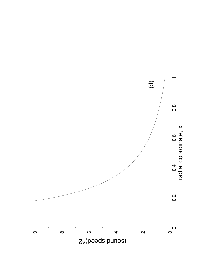
Figure 1: Plots of: (a) the metric functions $y^{2}$ and $z$; (b) the pressure $P$, the mass and charge densities $\kappa\rho$ and $\kappa\sigma$; (c) the mass and charge functions $m(r)$ and $q(r)$ and (d) $dP/d\rho$ for $b=0$.

The speed of sound in the fluid sphere is also of interest. This speed should be positive and causal, that is

$$0\leq\frac{dP}{d\rho}\leq 1.$$ (32)

Figure (1) is a plot of the speed of sound in this medium which indicates that the speed is certainly not causal in this case.

If this solution is matched to the extreme Reissner-Nordström solution, we impose the condition given in equation (31). Where $b=0$, the boundary $x_{0}$ is solved for:

$$x_{0}=\frac{1}{2}\frac{a^{2}}{(-c)}.$$

Unfortunately, this radial boundary also produces negative pressures over part of the fluid sphere. Figure (2) shows the example with

$$a = 1$$

$$c = -\frac{1}{6}$$

$$x_{0} = 1$$

Figure 2: Plots of: (a) the metric functions $y^{2}$ and $z$; (b) the pressure $P$, the mass and charge densities $\kappa\rho$ and $\kappa\sigma$; (c) the mass and charge functions $m(r)$ and $q(r)$ and (d) $dP/d\rho$ for the extreme Reissner-Nordström solution and $b=0$.

The speed of sound is singular at the center of the sphere and decreases when both the pressure and mass density are decreasing The speed is negative when the pressure increases. The speed is plotted in Figure (2).

If we impose the condition $\rho(x_{0})=0$, the boundary of the fluid sphere is

$$x_{0}=\sqrt{\frac{\rho_{0}}{\rho_{2}}}=\sqrt{\frac{3a}{8(-c)}}$$

and equation (26) implies

$$C_{2}=\frac{a}{16}.$$

The junction condition (25) produces

$$C_{1}=\sqrt{z(x_{0})}-\frac{a}{16}\xi_{0}.$$

In this case, the pressure, from equation (23), reads

$$\kappa P=4\sqrt{z}\left(\frac{C_{2}}{C_{1}+C_{2}\xi}\right)-a-2cx^{2}.$$ (33)

The pressure will be positive at the center ($x=\xi=0$) so long as $C_{1}<\frac{1}{4}$. Unfortunately, having the two conditions on the pressure, that the pressure is positive at the center and vanishes at the boundary, is not sufficient to prove that this is a positive pressure case. Numerical evaluation of the pressure shows that it has an additional point between the center and the boundary at which it goes to zero. That is, the pressure starts positive, then becomes negative before vanishing at the boundary. We illustrate a particular example of this behavior in Figure (3) with the following values for the constants $a$ and $c$:

$$a = 1$$

$$c = -\frac{1}{6}$$

Figure 3: Plots of: (a) the metric functions $y^{2}$ and $z$; (b) the pressure $P$, the mass and charge densities $\kappa\rho$ and $\kappa\sigma$; (c) the mass and charge functions $m(r)$ and $q(r)$ and (d) $dP/d\rho$ for $b=0$ and $\rho(x_{0})=0$.

3.2 Case $d<0$ ($b>0$, $\rho_{1}<0$)

This case involves the real exponential solution for $y$ given by equation (20). If we do not impose the condition that the mass density goes to zero at the boundary, we can solve for the constants $C_{1}$ and $C_{2}$ using the junction condition (25) and equation (27). These two equations result in

$$C_{1} = \frac{1}{2}e^{-\sqrt{-d}\xi_{0}}\left[\sqrt{z(x_{0})}+\frac{1}{\sqrt{-d}}\left(\frac{a}{4}+\frac{b}{4}x_{0}+\frac{c}{2}x_{0}^{2}\right)\right]$$

$$C_{2} = \frac{1}{2}e^{\sqrt{-d}\xi_{0}}\left[\sqrt{z(x_{0})}-\frac{1}{\sqrt{-d}}\left(\frac{a}{4}+\frac{b}{4}x_{0}+\frac{c}{2}x_{0}^{2}\right)\right]$$

These constants do give positive pressures as shown in the following example. Choose the following values for the constants $a$, $b$, $c$, and $x_{0}$:

$$a = 1$$

$$b = 1$$

$$c = -2$$

$$x_{0} = 0.09$$

Our results are shown in Figure (4).

Figure 4: Plots of: (a) the metric functions $y^{2}$ and $z$; (b) the pressure $P$, the mass and charge densities $\kappa\rho$ and $\kappa\sigma$; (c) the mass and charge functions $m(r)$ and $q(r)$ and (d) $dP/d\rho$ for $b>0$.

Once again, the speed of sound in this medium $\frac{dP}{d\rho}$ is evaluated and, as shown in Figure (4), is negative for this case. This is due to the fact that the mass density increases over the range of interest while the pressure decreases.

A match to the extreme Reissner-Nordström solution leads to a boundary given by the solution to equation (31):

$$x_{0}=\left(\frac{\sqrt{-c}}{b}\pm\frac{1}{b}\sqrt{-c-ab}\right)^{2}$$

where the minus sign case is chosen to ensure that the mass density remains positive over the region of the fluid sphere. Using the same values for the other constants as the previous example, Figure (5) is obtained.

Figure 5: Plots of: (a) the metric functions $y^{2}$ and $z$; (b) the pressure $P$, the mass and charge densities $\kappa\rho$ and $\kappa\sigma$; (c) the mass and charge functions $m(r)$ and $q(r)$ and (d) $dP/d\rho$ for extreme Reissner-Nordström solution and $b>0$.

The speed of sound becomes singular when $d\rho=0$.

If the mass density is forced to go to zero at the boundary of the fluid sphere ($\rho(x_{0})=0$), we solve for the boundary:

$$x_{0} = -\frac{\rho_{1}}{2\rho_{2}}+\frac{1}{2\rho_{2}}\sqrt{\rho_{1}^{2}+4\rho_{0}\rho_{2}}$$

$$= \frac{5b}{16(-c)}+\frac{1}{16(-c)}\sqrt{25b^{2}+96a(-c)}$$

The two conditions given by equations (25) and (26) allow us to solve for the constants $C_{1}$ and $C_{2}$,

$$C_{1} = \frac{1}{2}e^{-\sqrt{-d}\xi_{0}}\left[\sqrt{z(x_{0})}+\frac{z_{x}(x_{0})}{2\sqrt{-d}}\right]$$

$$C_{2} = \frac{1}{2}e^{\sqrt{-d}\xi_{0}}\left[\sqrt{z(x_{0})}-\frac{z_{x}(x_{0})}{2\sqrt{-d}}\right]$$

The pressure, from equation (23), is now

$$\kappa P=4\sqrt{-dz}\left(\frac{C_{1}e^{\sqrt{-d}\xi}-C_{2}e^{-\sqrt{-d}\xi}}{C_{1}e^{\sqrt{-d}\xi}+C_{2}e^{-\sqrt{-d}\xi}}\right)-a-bx-2cx^{2}$$ (35)

The condition for the pressure to be positive at the center of the fluid sphere is

$$\frac{C_{1}-C_{2}}{C_{1}+C_{2}}>\frac{a}{2\sqrt{b}}.$$

This clearly requires $C_{1}>C_{2}$ but this sets no clear condition on $z_{x}\left(x_{0}\right)$ due to the presence of the real exponentials in $C_{1}$ and $C_{2}$. The pressures appear to be negative when the contribution from the charge overwhelms the contribution from the mass, especially near the boundary where the mass density is virtually nil. The constants $a$, $b$, and $c$ are the same as in the previous example while $x_{0}$ is now given by equation (3.2). Figure (6) shows this negative pressure case.

Figure 6: Plots of: (a) the metric functions $y^{2}$ and $z$; (b) the pressure $P$, the mass and charge densities $\kappa\rho$ and $\kappa\sigma$; (c) the mass and charge functions $m(r)$ and $q(r)$ and (d) $dP/d\rho$ for $b>0$ and $\rho(x_{0})=0$.

The speed of sound in this case becomes singular at the point of maximum mass density (where $d\rho=0$).

We can also investigate the sub-case of $\rho_{0}=0$ with both conditions on $\rho(x_{0})$. Thus, both the mass and charge densities are zero at the center of the fluid sphere. This is the only relevant case in which to examine this sub-case as the mass density will remain positive for a large enough choice of $\rho_{1}$. When $\rho(x_{0})>0$ we desire the mass density to be large relative to the charge density, so the following values for the constants $a$, $b$, $c$, and $x_{0}$ are chosen:

$$a = 0$$

$$b = 10$$

$$c = -2$$

$$x_{0} = 0.3$$

We do in fact obtain positive pressures as shown in Figure (7).

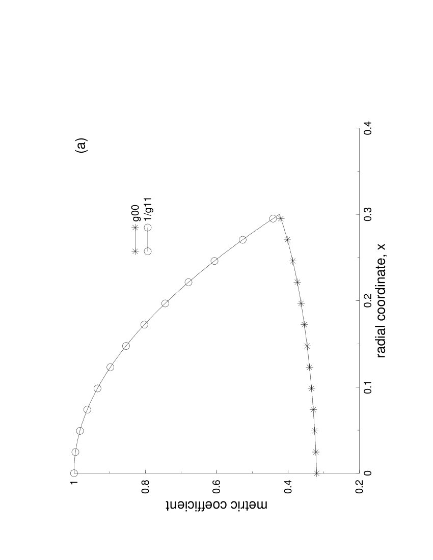
Figure 7: Plots of: (a) the metric functions $y^{2}$ and $z$; (b) the pressure $P$, the mass and charge densities $\kappa\rho$ and $\kappa\sigma$; (c) the mass and charge functions $m(r)$ and $q(r)$ and (d) $dP/d\rho$ for $a=0$ and $b>0$.

The speed of sound in this case remains negative due to the increasing mass density with a decreasing pressure. The speed is shown in Figure (7).

The extreme Reissner-Nordström solution has a boundary given from equation (31) of:

$$x_{0}=\frac{4(-c)}{b^{2}}$$

This leads to negative pressures over part of the sphere as in the example given in Figure (8) where the following values for the constants are used

$$a = 0$$

$$b = 7$$

$$c = -2$$

Figure 8: Plots of: (a) the metric functions $y^{2}$ and $z$; (b) the pressure $P$, the mass and charge densities $\kappa\rho$ and $\kappa\sigma$; (c) the mass and charge functions $m(r)$ and $q(r)$ and (d) $dP/d\rho$ for extreme Reissner-Nordström solution, $a=0$, and $b>0$.

The speed of sound in this case begins positive yet becomes negative as the pressure increases and then decreases. This speed is given in Figure (8).

However, when $\rho(x_{0})=0$ and $\rho_{0}=0$ the mass density remains below the charge density and, hence, negative pressures result. For example, we choose the following values for $b$ and $c$:

$$b = 2$$

$$c = -2.$$

The resulting pressure is shown in Figure (9).

Figure 9: Plots of: (a) the metric functions $y^{2}$ and $z$; (b) the pressure $P$, the mass and charge densities $\kappa\rho$ and $\kappa\sigma$; (c) the mass and charge functions $m(r)$ and $q(r)$ and (d) $dP/d\rho$ for $a=0$, $b>0$, and $\rho(x_{0})=0$.

Figure 10: Plots of: (a) the metric functions $y^{2}$ and $z$; (b) the pressure $P$, the mass and charge densities $\kappa\rho$ and $\kappa\sigma$; (c) the mass and charge functions $m(r)$ and $q(r)$ and (d) $dP/d\rho$ for $b<0$.

The speed of sound in this case becomes singular when the mass density peaks (i.e. $d\rho=0$).

3.3 Case $d>0$ ($b<0$, $\rho_{1}>0$)

This case involves the sine and cosine solution for $y$ given by equation (21). Now, if we use the junction condition (25) and equation (27), the constants $C_{1}$ and $C_{2}$ become

$$C_{1} = \sqrt{z(x_{0})}\sin\sqrt{\frac{b}{4}}\xi_{0}+\frac{1}{\sqrt{b}}\left(\frac{a}{2}+\frac{b}{2}x_{0}+cx_{0}^{2}\right)\cos\sqrt{\frac{b}{4}}\xi_{0}$$

$$C_{2} = \sqrt{z(x_{0})}\cos\sqrt{\frac{b}{4}}\xi_{0}-\frac{1}{\sqrt{b}}\left(\frac{a}{2}+\frac{b}{2}x_{0}+cx_{0}^{2}\right)\sin\sqrt{\frac{b}{4}}\xi_{0}.$$

We obtain positive pressures in this case as well. The following example, Figure(10), uses the following values for the constants $a$, $b$, $c$, and $x_{0}$:

$$a = 1$$

$$b = -1$$

$$c = -2$$

$$x_{0} = 0.05$$

The speed of sound in this case, as shown in Figure (10), does follow the conditions given by equation (32).

Thus, this case satisfies the conditions for a physically realistic solution, that: at the center of the sphere, the mass $m$ vanishes and $e^{\lambda}=1$; the metric functions $y^{2}$ and $z$ match the external Reissner-Nordström metric at the boundary; the pressure is positive and monotonically goes to zero at the boundary; the mass density is positive; and the speed of sound in this medium is both positive and causal.

Matching to the extreme Reissner-Nordström solution results in another situation where the pressure does not monotonically vanish at the boundary, given in Figure (11) for the same values as in the last example. The boundary is given from equation (31):

$$x_{0}=\left(\frac{\sqrt{-c}}{b}-\frac{1}{b}\sqrt{-c-ab}\right)^{2}.$$

Figure 11: Plots of: (a) the metric functions $y^{2}$ and $z$; (b) the pressure $P$, the mass and charge densities $\kappa\rho$ and $\kappa\sigma$; (c) the mass and charge functions $m(r)$ and $q(r)$ and (d) $dP/d\rho$ for extreme Reissner-Nordström solution and $b<0$.

Figure 12: Plots of: (a) the metric functions $y^{2}$ and $z$; (b) the pressure $P$, the mass and charge densities $\kappa\rho$ and $\kappa\sigma$; (c) the mass and charge functions $m(r)$ and $q(r)$ and (d) $dP/d\rho$ for $b<0$ and $\rho(x_{0})=0$.

The speed of sound is fractional but does not remain positive as illustrated in Figure (11).

The condition that the mass density goes to zero yields the boundary

$$x_{0} = -\frac{\rho_{1}}{2\rho_{2}}+\frac{1}{2\rho_{2}}\sqrt{\rho_{1}^{2}+4\rho_{0}\rho_{2}}$$

$$= \frac{5b}{16(-c)}+\frac{1}{16(-c)}\sqrt{25b^{2}+96a(-c)}.$$

The junction condition (25) and equation (26) are used to solve for the constants $C_{1}$ and $C_{2}$:

$$C_{1} = \sqrt{z(x_{0})}\sin\sqrt{d}\xi_{0}+\frac{z_{x}(x_{0})}{2\sqrt{d}}\cos\sqrt{d}\xi_{0}$$

$$C_{2} = \sqrt{z(x_{0})}\cos\sqrt{d}\xi_{0}-\frac{z_{x}(x_{0})}{2\sqrt{d}}\sin\sqrt{d}\xi_{0}.$$

The pressure, from equation (23), is given by

$$\kappa P=4\sqrt{dz}\left(\frac{C_{1}\cos\sqrt{d}\xi-C_{2}\sin\sqrt{d}\xi}{C_{1}\sin\sqrt{d}\xi+C_{2}\cos\sqrt{d}\xi}\right)-a-bx-2cx^{2}.$$ (36)

The condition that the pressure be positive at the center leads to the relation

$$\frac{C_{1}}{C_{2}}>\frac{a}{4\sqrt{d}},$$

which is not satisfied, in general. We show an example in Figure (12)with negative pressures where the following values were used

The speed of sound in this case, begins at a positive fractional value but decreases through zero to negative values as the pressure first decreases and then increases to zero at the boundary.

Finally One might ask which solutions (of the 127

4 Conclusions

It has been shown that by giving the mass density and charge aspect functions explicitly was fourth-order polynomials in the curvature radial coordinate leads to a simple linear second-order differential equation with constant coefficients that can be easily solved. With an appropriate choice of the constants appearing in the polynomial, some of the solutions can be made to satisfy the requirements for begin physically acceptable. Given the small number of known solutions for both charged and neutral fluid spheres that obey such criteria, the configurations of charge and mass found in these solutions may be expected to form from a realistic collapse to a condensed spherical object.

While matching to the external Reissner-Nordstrom solution causes no problems since this only determines the values for the constants of integration, it has been shown that with this family of solutions it is impossible to find realistic configurations that lead to extreme Reissner-Nordstrom solutions. In all cases where the solution was matched to the extreme Reissner-Nordstrom vacuum solution, problems arose in maintaining a speed of sound that is bounded by the speed of light.

It remains to be determined how stable these configurations are, and this will be studied in the future. Given that the equation of state for the fluid has not been written in the form $p=p(\rho)$ does make the stability analysis a bit more difficult since it is not known if one can use adiabaticity arguments without directly checking them independently. However a general stability analysis of this and other known exact solutions should be interesting from the point of view of trying to understand what charged fluid configurations could possibly be formed from the gravitational collapse of material that has an excess charge density.

Finally, one should be able to extend this method to other explicit functions for both the mass density and charge aspect. Higher order polynomials are expected to produce similar results and one can expect that these would force more of the charge to be distributed closer to the surface of the sphere. Further studies on what the most general polynomials might be and the relationships between the charge and mass distributions will be studied in the future.

4.1 Acknowledgments

DH would like to thank D. Giang for discussions concerning methods for solving the Einstein-Maxwell system of equations. This research was funded through an NSERC (Canada) Discovery Grant.

5 References

• S.D. Majumdar, Phys. Rev., 72, 390 (1947).

• A. Papapetrou, Proc. Roy. Irish Acad., A 51, 191 (1947).

• B.V. Ivanov, Phys. Rev. D 65, 104001, (2002).

• M.S.R. Delgaty and K. Lake, Comput. Phys. Commun. 115, 395, (1998) [arXiv:gr-qc/9809013].

• M.R. Finch and J.E.F. Skea, unpublished preprint,
  www.dft.if.euerj.br/users/Jim_Skea/papers/pfrev.ps.

• R.C. Tolman, Phys. Rev.  55, 363, (1939).

• S. Bayin, Phys. Rev. D 18, 2745, (1975).