Partha Konar1, Kyoungchul Kong2, Konstantin T. Matchev1, and Myeonghun Park11Physics Department, University of Florida, Gainesville, FL 32611, USA2Theoretical Physics Department, SLAC, Menlo Park, CA 94025
(19 March, 2010)
Abstract
We propose a new model-independent technique for mass measurements in
missing energy events at hadron colliders. We illustrate our method with
the most challenging case of a short, single-step decay chain.
We consider inclusive same-sign chargino pair production in supersymmetry,
followed by leptonic decays to sneutrinos:
().
We introduce two one-dimensional decompositions of the Cambridge
variable:
and , on the direction of the upstream
transverse momentum and the direction orthogonal to it, respectively.
We show that the sneutrino mass can be measured directly by
minimizing the number of events in which
exceeds a certain threshold, conveniently measured from the endpoint
.
pacs:
14.80.Ly,12.60.Jv,11.80.Cr
The Large Hadron Collider (LHC) at CERN has begun its long awaited
exploration of the TeV scale, where new physics beyond the Standard Model (SM)
may hold the key to our understanding of some very basic questions about
our universe: What is the dark matter? What are the fundamental symmetries
of Nature? Are there any hidden dimensions of space? A potential
discovery of a missing energy signal at the LHC may
relate to all three of these questions, if the missing energy is
due to a stable, neutral, weakly interacting massive
particle in a theory with space-time supersymmetry (SUSY) Chung:2003fi
or extra dimensions Hooper:2007qk.
The first order of business after the discovery of a
missing energy signal at the LHC will be to measure
the mass of the missing particle and prove that it is
not simply a SM neutrino Chang:2009dh.
This deceptively simple task turned out to be
a notoriously difficult challenge.
The generic topology of a prototypical “SUSY-like” missing energy event
is schematically depicted in Fig. 1.
Figure 1: The generic event topology under consideration.
All particles visible in the detector are clustered into three groups:
upstream objects with total transverse momentum ,
and two composite visible particles , each with invariant mass
and total transverse momentum . The transverse momenta of the
two missing particles are labelled by .
Consider inclusive production of an identical pair of
new particles (from now on referred to as “parents”).
Each parent decays semi-invisibly to a set of SM
particles , (), which are visible in the detector,
and a dark matter particle (from now on referred to as the “child”)
which escapes detection.
In general, the parent pair may be accompanied by
a number of additional “upstream” objects (typically jets)
with total transverse momentum . They
may originate from various sources such as initial state radiation
or decays of even heavier particles up the decay chain.
We shall not be interested in the exact details of the
physics responsible for , adopting a fully inclusive approach
to the production of the parents . Given this general setup,
the goal is to determine independently the mass of the parent
and the mass of the child.
In the past, several approaches to this problem have been proposed,
e.g. invariant mass endpoint measurements imass
or exact reconstruction of the missing particle momenta exactreco. Unfortunately, they only apply to sufficiently long
decay chains, where the visible particles in arise from
a sequence of at least three 2-body decays Burns:2008va.
In the simplest example of a short, single-step decay chain, each consists
of a single SM particle of fixed mass , and neither of these
two approaches will work.
One must then resort to methods
based on the Cambridge variable approxreco; kink; Matchev:2009fh
or the related Sheffield variable Tovey:2008ui; Matchev:2009ad.
Unfortunately, in order to apply those techniques, one must
work with a subset of events within a relatively narrow fixed
range, incurring some loss in statistics.
In this Letter we propose a new method which
uses the full data set, with no such loss in statistics.
Our method is based on the “subsystem” variant Matchev:2009fh
of the original variable approxreco.
For any given event, one can construct the transverse mass
of each parent :
(1)
where
(2)
is the transverse energy of the visible particle
and child particle in each branch of Fig. 1,
correspondingly. The individual momenta
of the missing child particles are unknown, but
they are constrained by the measured missing transverse
momentum in the event:
(3)
For the true values of the missing momenta ,
each transverse mass in (1) is bounded from
above by the true parent mass . This fact can be used
in a rather ingenious way to define the Cambridge
variable approxreco. One takes the larger of the two
quantities in (1) and minimizes it over
all possible partitions of the unknown children momenta
, subject to the constraint (3):
(4)
For a given , the endpoint of this distribution
gives the parent mass as a function of the input
trial child mass :
(5)
This property
provides one relation among the two unknown
masses and approxreco.
Here we propose to obtain a second relation by using
the property that
the function
is independent of at the true child mass :
(6)
which we can rewrite more informatively as
(7)
with equality being achieved only for .
Eq. (7) implies that,
for any given , there will always be a certain
number of events whose values will exceed the
reference value , unless the trial mass
happens to coincide with the true child mass .
In order to quantify this effect, we define the function
(8)
where is the Heaviside step function.
From the definition of
it is clear that it is minimized at ,
where in theory we would expect
(9)
In reality, the value of will be lifted from 0, due to
finite particle width effects, detector resolution, etc.
Nevertheless we expect that the location of the
minimum will still be at ,
allowing a direct measurement of the child mass :
(10)
which is our first main result.
Once the child mass is found from (10),
the true parent mass is obtained as usual from (5)
as .
At this point it is not clear whether we have gained anything
statistics-wise, since the reference quantity
appearing in the definition (8) has to be
measured at a fixed anyway. Our second main result
in this paper is that can in fact
be measured from the full data set with no loss in statistics
as follows.
Let us introduce one-dimensional (1D)
decompositions of onto the two special directions
defined by the upstream momentum vector .
Following Ref. Matchev:2009ad, first project the visible
transverse momenta of Fig. 1
onto the direction () and its orthogonal direction
():
(11)
(12)
and similarly for the two transverse momenta
of the children and for . Now consider the corresponding 1D decompositions
of the transverse parent masses (1)
Now we define 1D decompositions
in complete analogy with the standard definition
(4):
(21)
(30)
These decompositions
are extremely useful. For once, the 1D variables
(21,30) can be calculated
via simple analytic expressions as shown below. In contrast,
a general formula for the original variable (4)
in the presence of arbitrary
is unknown and one still has to compute
numerically Cheng:2008hk.
More importantly,
allows us to measure the reference quantity
in (8)
from the full data set, using events with any
value of .
To understand the basic idea,
it is sufficient to consider the simplest, yet most
challenging case of a single step decay chain. Let
be a single,
(approximately) massless SM particle: .
(The discussion for the massive case proceeds analogously.)
In what follows, for illustration we shall use the
same-sign dilepton channel in supersymmetry, where
each is a lepton resulting from a chargino decay
to a sneutrino Matchev:2009fh. The charginos themselves
are produced indirectly in the decays of squarks and gluinos.
For concreteness we shall use a SUSY spectrum given by the LM6 CMS
study point Ball:2007zza.
At point LM6, the chargino (sneutrino) mass is
GeV ( GeV), and the rest of the
SUSY mass spectrum can be found in Ball:2007zza.
In our simulations we use the PYTHIA event generator Sjostrand:2006za
and the PGS detector simulation program PGS.
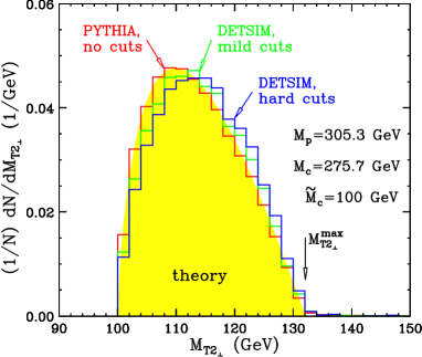
Figure 2: The unit-normalized distribution
(35) for the same-sign dilepton channel in a SUSY model with
LM6 CMS mass spectrum and a choice of test mass GeV.
The yellow shaded distribution shows the theoretically predicted shape (35),
matching very well the parton level result from PYTHIA with no cuts (red histogram).
The green (blue) histogram is the corresponding result after
PGS detector simulation with mild
(hard) cuts as explained in the text.
The endpoint expected from eq. (32) is GeV
and is marked with the vertical arrow.
The variable has several unique properties.
Eventwise, it can be calculated analytically as
(31)
The endpoint of the
distribution is given by
(32)
in terms of the parameter introduced in Burns:2008va
(33)
Eq. (32) reveals perhaps the most important
feature of the variable: its endpoint is
independent of the upstream and can thus
be measured with the whole data sample.
We can even predict analytically the
shape of the (unit-normalized)
differential distribution
(34)
where
is the fraction of events in the lowest bin
, while the shape of the remaining (unit-normalized)
distribution is given by (see Fig. 2)
(35)
Notice that this shape
does not depend on any unknown kinematic parameters,
such as the unknown center-of-mass energy
or longitudinal momentum of the initial hard scattering.
It is also insensitive to spin correlation effects, whenever the
upstream momentum results from production and/or decay
processes involving scalar particles (e.g. squarks) or
vectorlike couplings (e.g. the QCD gauge coupling).
It is even independent of
the actual value of the upstream momentum
. Thus we are not restricted to a particular range and can use
the whole event sample in the analysis.
For any choice of (in Fig. 2 we used
GeV), eq. (35) is a one-parameter curve
which can be fitted to the data to obtain the parameter and
from there the endpoint (32).
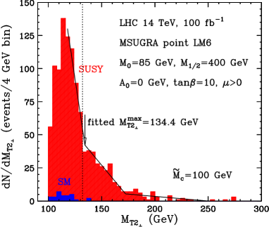
Figure 3: Observable distribution
after hard cuts for 100 fb-1 of LHC data. The total stacked distribution
consists of the SUSY signal (red) and the SM background (blue).
The solid line is the result of a simple linear fit, revealing
endpoints at 134.4 GeV and 172.4 GeV.
As always, there are practical limitations to the use of
such shape fitting. First, the shape (35) is modified in the presence of “mild” cuts,
which are required for lepton identification in PGS
(green histogram in Fig. 2),
and more importantly, for the discovery of the same-sign
dilepton SUSY signal over the SM backgrounds.
To ensure discovery, we use “hard” cuts
as follows
Ball:2007zza; Pakhotin:2006wx: exactly
two isolated leptons with GeV,
at least three jets with GeV,
GeV and a veto on tau jets.
With those cuts, in the dimuon channel alone, the
remaining SM background cross-section is
dominated by and is just 0.15 fb, while
the SUSY signal is 14 fb, leading to a
discovery with just
of data Ball:2007zza; Pakhotin:2006wx.
The distortion of the shape with these
hard offline cuts is illustrated by the blue
(rightmost) histogram in Fig. 2.
The actual distribution which we expect to
observe with of data, is shown
in Fig. 3 and is comprised of a relatively small
SM background component (blue) and a dominant SUSY signal
component (red). In spite of the presence of a sizable
SUSY combinatorial background, the endpoint
expected from Fig. 2 is clearly visible
and its location from a simple linear fit is obtained as
134.4 GeV, which is very close to the nominal value of
132.1 GeV. (Interestingly, the data reveals a second endpoint at
172.4 GeV, which is due to events in which one
chargino decays through a charged slepton:
Matchev:2009fh.
Its nominal value is 169.2 GeV.)
Our final key observation is that
(36)
which allows to rewrite
the function of eq. (8) as
(37)
The analysis just described
allows a very precise measurement of the
benchmark quantity
appearing in (37), so that the function
itself can be reliably reconstructed,
using the whole event sample all the way
throughout the analysis, without any loss in statistics.
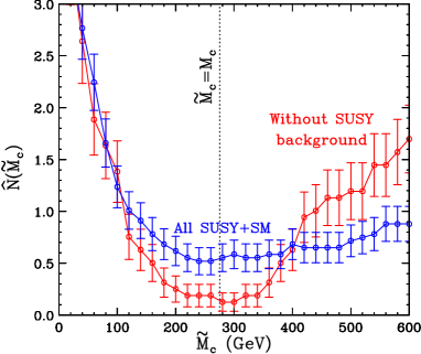
We show our result in Fig. 4, where for convenience we
unit-normalize the function as
(38)
where the averaging is performed over the plotted range of .
Figure 4: The function
defined in (38). The blue (red)
set of measurements are with (without)
SUSY combinatorial background.
The error bars shown are purely statistical.
As expected, the function
exhibits a minimum in the vicinity of the true
sneutrino mass GeV.
Ignoring the SUSY combinatorial background,
this measurement (red data points) is quite precise,
at the level of a few percent. In order to reduce the combinatorial
background, we select events with
and veto very hard111The
measured value of in Fig. 3
already implies that the mass splitting is on the order of
30 GeV, resulting in a rather soft lepton spectrum. leptons
with GeV. The resulting measurement
(blue data points) is at the level of .
This precision is clearly sufficient
to exclude SM neutrinos as the source of the missing energy,
hinting at a potential dark matter discovery at the LHC.
In conclusion, we summarize the novel features and advantages of our method
in comparison to previous -based proposals in the literature
kink; Matchev:2009fh. First, we make crucial use of
property (6), which allowed us to
measure directly the missing particle mass as
in eq. (10). Second, both the benchmark quantity
entering eq. (37)
as well as the the function itself
can be measured using the whole available data sample
at any.
To the extent that the definition of relies only
on the direction and not the magnitude of the upstream ,
our method is insensitive to the jet energy scale error Matchev:2009ad.
We have also provided exact analytical formulas for the computation
of the 1D decomposed variables222The corresponding
analytical results for can be found in the first
version of this paper, which is available on the hep-ph archive.
and the shape (35) of the distribution.
Acknowledgments. We thank L. Pape for useful comments.
This work is supported in part by
US Department of Energy grants DE-FG02-97ER41029 and DE-AC02-76SF00515.
References
(1)
See, e.g. D. Chung et al., Phys. Rept. 407, 1 (2005).
(2)
D. Hooper and S. Profumo,
Phys. Rept. 453, 29 (2007).
(3)
S. Chang and A. de Gouvea,
Phys. Rev. D 80, 015008 (2009).
(4)
I. Hinchliffe et al., Phys. Rev. D 55, 5520 (1997);
B. C. Allanach, C. G. Lester, M. A. Parker and B. R. Webber,
JHEP 0009, 004 (2000);
B. K. Gjelsten, D. J. Miller and P. Osland,
JHEP 0412, 003 (2004);
D. Costanzo and D. R. Tovey,
JHEP 0904, 084 (2009);
M. Burns, K. T. Matchev and M. Park,
JHEP 0905, 094 (2009);
K. T. Matchev, F. Moortgat, L. Pape and M. Park,
JHEP 0908, 104 (2009).
(5)
K. Kawagoe, M. Nojiri and G. Polesello,
Phys. Rev. D 71, 035008 (2005);
H. C. Cheng et al., JHEP 0712, 076 (2007);
M. Nojiri, G. Polesello and D. R. Tovey,
JHEP 0805, 014 (2008);
H. C. Cheng et al., Phys. Rev. Lett. 100, 252001 (2008);
B. Webber,
JHEP 0909, 124 (2009).
(6)
M. Burns, K. Kong, K. T. Matchev and M. Park,
JHEP 0903, 143 (2009).
(7)
C. Lester and D. Summers,
Phys. Lett. B 463, 99 (1999);
A. Barr, C. Lester and P. Stephens,
J. Phys. G 29, 2343 (2003).
(8)
W. Cho, K. Choi, Y. Kim and C. Park,
Phys. Rev. Lett. 100, 171801 (2008);
JHEP 0802, 035 (2008);
B. Gripaios,
JHEP 0802, 053 (2008);
A. Barr, B. Gripaios and C. Lester,
JHEP 0802, 014 (2008).
(9)
K. T. Matchev, F. Moortgat, L. Pape and M. Park,
arXiv:0909.4300 [hep-ph].
(10)
D. R. Tovey,
JHEP 0804, 034 (2008);
G. Polesello and D. R. Tovey,
arXiv:0910.0174 [hep-ph].
(11)
K. T. Matchev and M. Park,
arXiv:0910.1584 [hep-ph].
(12)
H. C. Cheng and Z. Han,
JHEP 0812, 063 (2008).
(13)
G. L. Bayatian et al., J. Phys. G 34, 995 (2007).
(14)
T. Sjostrand, S. Mrenna and P. Skands,
JHEP 0605, 026 (2006).